4DVAR assimilation of GNSS zenith path delays and precipitable water into a numerical weather prediction model WRF - Atmos. Meas. Tech
←
→
Page content transcription
If your browser does not render page correctly, please read the page content below
Atmos. Meas. Tech., 12, 345–361, 2019
https://doi.org/10.5194/amt-12-345-2019
© Author(s) 2019. This work is distributed under
the Creative Commons Attribution 4.0 License.

4DVAR assimilation of GNSS zenith path delays and precipitable
water into a numerical weather prediction model WRF
Witold Rohm1 , Jakub Guzikowski2 , Karina Wilgan1,4 , and Maciej Kryza3
1 Institute of Geodesy and Geoinformatics, Wrocław University of Environmental and Life Sciences, Wrocław, 50-357, Poland
2 Institute of Geophysics, Polish Academy of Sciences, 01-452 Warsaw, Poland
3 Institute of Geography and Regional Development, University of Wrocław, Wrocław, 50-137, Poland
4 Institute of Geodesy and Photogrammetry, ETH Zürich, Zürich, 8093, Switzerland

Correspondence: Witold Rohm (witold.rohm@upwr.edu.pl)

Received: 3 August 2018 – Discussion started: 17 August 2018
Revised: 10 December 2018 – Accepted: 11 December 2018 – Published: 18 January 2019

Abstract. The GNSS data assimilation is currently widely           RS and SYNOP; ZTD alone; and finally ZTD, with RS and
discussed in the literature with respect to the various ap-        SYNOP for 5–23 May 2013, and (3) assimilation of PW or
plications for meteorology and numerical weather models.           ZTD during severe weather events in June 2013. Once the
Data assimilation combines atmospheric measurements with           initial conditions were established, the forecast was run for
knowledge of atmospheric behavior as codified in computer          24 h.
models. With this approach, the “best” estimate of current            The major conclusion of this study is that for all analyzed
conditions consistent with both information sources is pro-        cases, there are two parameters significantly changed once
duced. Some approaches also allow assimilating the non-            GNSS data are assimilated in the WRF model using GP-
prognostic variables, including remote sensing data from           SPW operator and these are moisture fields and rain. The
radar or GNSS (global navigation satellite system). These          GNSS observations improves forecast in the first 24 h, with
techniques are named variational data assimilation schemes         the strongest impact starting from a 9 h lead time. The rela-
and are based on a minimization of the cost function, which        tive humidity forecast in a vertical profile after assimilation
contains the differences between the model state (back-            of ZTD shows an over 20 % decrease of mean error start-
ground) and the observations. The variational assimilation is      ing from 2.5 km upward. Assimilation of PW alone does not
the first choice for data assimilation in the weather forecast     bring such a spectacular improvement. However, combina-
centers, however, current research is consequently looking         tion of PW, SYNOP and radiosonde improves distribution
into use of an iterative, filtering approach such as an extended   of humidity in the vertical profile by maximum of 12 %.
Kalman filter (EKF).                                               In the three analyzed severe weather cases PW always im-
   This paper shows the results of assimilation of the GNSS        proved the rain forecast and ZTD always reduced the humid-
data into numerical weather prediction (NWP) model WRF             ity field bias. Binary rain analysis shows that GNSS param-
(Weather Research and Forecasting). The WRF model offers           eters have significant impact on the rain forecast in the class
two different variational approaches: 3DVAR and 4DVAR,             above 1 mm h−1 .
both available through the WRF data assimilation (WRFDA)
package. The WRFDA assimilation procedure was modified
to correct for bias and observation errors. We assimilated
the zenith total delay (ZTD), precipitable water (PW), ra-         1   Introduction
diosonde (RS) and surface synoptic observations (SYNOP)
using a 4DVAR assimilation scheme. Three experiments               The data assimilation in weather forecasts is one of the key
have been performed: (1) assimilation of PW and ZTD for            components in all prediction systems as it is an initial value
May and June 2013, (2) assimilation of PW alone; PW, with          problem and the quality of the initial field has a large impact
                                                                   on the forecasts. Currently, the leading weather agencies as-

Published by Copernicus Publications on behalf of the European Geosciences Union.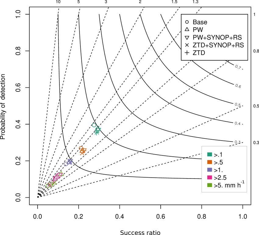
346                                                       W. Rohm et al.: 4DVAR assimilation of GNSS zenith path delays

similate operationally dozens of observation data types such     and RUC 40 km (Benjamin et al., 2002) or currently opera-
as radiosonde (RS) profiles, radiances from satellite observa-   tional rapid refresh (RAP) (Benjamin et al., 2016) that are
tions, SYNOPs, refractivities from radio occultations, pilot     targeting short 12 and 24 h predictions for decision making
reports and many others (Barker et al., 2004). With the advent   and safety operations with a large number of observations as-
of European Cooperation in Science & Technology (COST)           similated every hour. One of the first experiments using GPS
actions 716 (1999–2004), 1206 (2013–2017), as well as the        precipitable water (PW) in nowcasting service in the USA
project funded in the fifth framework program “Targeting         (RUC model 60 km) (Smith et al., 2000), showed a 1 % im-
Optimal Use of GPS Humidity Measurements in Meteorol-            provement of the relative humidity forecast in the bottom part
ogy” (TOUGH), the adoption of the ground based global            of the atmosphere. However, in specific cases related to ac-
navigation satellite systems (GNSS) observations to the op-      tive frontal weather, the improvement was much larger: 14 %
erational forecasts by most of the weather services in Europe    in the moistening and 24 % in the drying stage of the ad-
become a fact. In this study the term GNSS covers all nav-       vection. The increased spatial resolution to 20 km of RUC20
igation systems used world-wide, whereas the term Global         (Smith et al., 2007) shows stronger improvements in humid-
Positioning System (GPS) is related to only one source of        ity field and convective available potential energy, CAPE,
observations – the US based GPS. There are many publica-         than with RUC40. The 850 hPa relative humidity (RH) fore-
tions related to either (1) performance of large-scale weather   casts improve more in the nighttime, and in the colder season
forecast systems augmented with many observations includ-        than that in the warmer season. The current RAP model, run-
ing GNSS, (2) added value of GNSS observations in now-           ning on a 13km grid, continuously assimilates GPS PW every
casting services, or (3) case-based studies showing the im-      hour from 300 stations across the US (Benjamin et al., 2016).
pact of GNSS data in particular cases. The following three       It shows that there is clear benefit in using GPS observations,
approaches are discussed below.                                  especially for short term (nowcasting) predictions.
   A very comprehensive study done by Poli et al. (2007)            The third type of studies that are appearing in the lit-
on the global forecast model Arpage using four dimensional       erature are case based, showing the impact of GNSS on
variational assimilation (4DVAR) shows that the impact of        particular weather events. One of the first to test the im-
GPS zenith total delay (ZTD) on forecasts is different in win-   pact of GPS based ZTD observations in Europe was Cucu-
ter (improving pressure), spring (reducing surface humid-        rull et al. (2004). The authors used the NCAR/Penn State
ity root mean square error) and summer (positive impact on       Mesoscale Model 5 (MM5) ZTD 3DVAR assimilation for
wind, geopotential and precipitation, negative on humidity).     a case of a snow storm on 14–15 December 2001 over the
A similar, very detailed study was done by Bennitt and Jupp      western Mediterranean Sea. They found that there are reduc-
(2012), where the authors discussed the operational assimi-      tions of root mean square error (RMSE) of wind by 1.7 %,
lation of GPS ZTD in MetOffice into the North Atlantic and       temperature by 4.1 % and surface humidity by 17.8 %. The
European 12 and 24 km model in spring, summer and au-            authors also noted that the forecasts work better if the ground
tumn. The results were mixed: for all cases the introduction     based automatic weather stations were used in the same as-
of GPS ZTD increased the humidity bias, however the im-          similation run. Another example of an early stage case-based
provements of clouds forecasts were observed. Bennitt and        research is the assimilation of GPS PW by Nakamura et
Jupp (2012) also identify no clear benefit of 4DVAR against      al. (2004) with a 4DVAR scheme into a mesoscale Japanese
3DVAR. Lindskog et al. (2017) in their study in the Nordic       Meterological Agency (JMA) model for summer intensive
countries of GNSS ZTD impact on forecasts, confirmed that        rain cases. The assimilation of GPS data improved the pre-
the forecasts are sensitive to thinning distance. Shorter dis-   cipitation location, but the statistics did not show large im-
tance between stations (below 100 km) leads to a larger hu-      provement. One of the first GPS 4DVAR ZTD studies in the
midity bias in the lower troposphere, which may explain the      US was by De Pondeca and Zou (2001), who ran assimi-
humidity bias in the Bennitt and Jupp (2012) solution. Lind-     lation of GPS observations in MM5 together with the wind
skog et al. (2017) showed that the humidity forecast is better   profiler data and radio acoustic sounding system (RASS) vir-
when the GNSS ZTD is assimilated with other meteorolog-          tual temperature. Five 12 h experiments for California’s De-
ical observations such as the Advanced Microwave Sound-          cember frontal system passage were performed. It was found
ing Unit (AMSU) or Infrared Atmospheric Sounding Inter-          that the ZTD assimilation corrects the underestimation of ac-
ferometer (IASI) radiances. The authors also showed that the     cumulated rain by 33.15 % and 25.08 % for 6 and 12 h re-
adopted bias correction strategy and GNSS ZTD estimation         spectively. Adding the wind profiler improves the forecast by
procedure have marginal impact on the forecasts. All studies     88.26 % and 32.53 % and adding further RASS observations
run in large weather forecasting systems suggests that the as-   increases the performance to 93.21 % and 50.58 %, respec-
similation of GNSS ZTD, either 3D or 4DVAR, on average           tively. In a more recent study by Boniface et al. (2009), the
has a mostly neutral impact on the forecast if the system is     GPS ZTD was assimilated (3DVAR) for 280 stations over
already saturated with meteorological observations.              15 days into the high-resolution (2.5 km) AROME model.
   Another branch of weather models are those used in now-       The results were positive for poorly predicted precipitation
casting, such as the (legacy) rapid update cycle RUC 20 km       and neutral for well predicted ones. More recently, Tilev-

Atmos. Meas. Tech., 12, 345–361, 2019                                               www.atmos-meas-tech.net/12/345/2019/
W. Rohm et al.: 4DVAR assimilation of GNSS zenith path delays                                                                   347

Tanriover and Kahraman (2014) studied the impact of the
GPS PW assimilation in the Weather Research and Forecast-
ing (WRF) model in a 2 day case of intense snowfall fore-
casts in the central Anatolia. The authors performed three
experiments: base run, cold start and cycling all with PW
3DVAR operator. Results show that the cycling assimila-
tion mode decreases the temperature and humidity biases,
whereas the cold start performs worse than the control run.
Saito et al. (2016) studied the impact of ensemble predic-
tion that did not produce enough precipitation. They found
that even downscaling from 10 to 2 km still does not improve
locations of precipitation’s cores. Finally, the 4DVAR PW
assimilation into a non-hydrostatic model improved the loca-
tion of scattered intensive rain. In summary, most of the liter-
ature reported a substantial increase in the quality of the fore-
cast of humidity, rain location and sometimes also the rain
accumulated total amount. Less significant improvement was
achieved for wind speed and temperature. All studies that
used additional observations, especially these resolving ver-
tical structure of the water vapor and temperature, comple-
mented GNSS observations and improved the forecast even
more.                                                               Figure 1. The WRF model configuration (the inner square repre-
   The literature review shows that the impact of the GNSS          sents the nested domain with 4 km × 4 km resolution). Colors de-
ZTD/PW assimilation depends on the number of already as-            note the orography of the terrain (m a.s.l.).
similated observations and applied preprocessing (Bennitt
and Jupp, 2012; Lindskog et al., 2017; Poli et al., 2007) as
well as on the type of weather conditions. The main aim of          2     Data
this paper is to quantify the impact of the GNSS data, both
ZTD and PW, gathered operationally in Poland, in weather            The GNSS PW/ZTD data are assimilated into the NWP WRF
forecasting. The study is based on the WRF model with a             model. The chosen period covers May and June 2013, with
high spatial resolution of 4 km × 4 km supported with the           a special focus on 5–23 May 2013 and three shorter cases:
WRF data assimilation (WRFDA) package. We show the im-              (a) 29–31 May, (b) 17–19 June and (c) 24–26 June 2013.
portance of the GNSS data assimilation for cases of various         The period is chosen in accordance with the COST Action
meteorological conditions observed in May and June 2013,            ES1206 GNSS meteorology benchmark (Douša et al., 2016).
which is a benchmark period for COST Action ES1206. To
our best knowledge, no GNSS ZTD/PW assimilation experi-             2.1    WRF model
ment was carried out in Poland yet. Moreover, we found only
one publication (Tilev-Tanriover and Kahraman, 2014) deal-          In this study the WRF model is used, it is numerical weather
ing with the assimilation of GPS ZTD and PW into widely             prediction system designated for simulation of multiscale,
adopted WRF model using the WRFDA package. We present               spatial and temporal atmosphere flows. The WRF configu-
a study showing the impact of GNSS ZTD and PW observa-              ration (Kryza et al., 2013) is based on two nested model
tions on the forecasts for a longer time period – 2 months          domains. The first domain covers the European area with
(May 2013 – calm weather conditions and June 2013 – ac-             a 12 km × 12 km grid spacing. The second, nested domain
tive stormy weather), followed by quantifying improvements          covers Poland and Central Europe with a 4 km × 4 km grid
of adding RS and SYNOP data into the assimilation system            spacing (Fig. 1).
already run with GNSS observations, and finally we veri-               Initial and boundary conditions are taken from the Na-
fied impact of GNSS observations on prediction for specific         tional Center for Environmental Prediction Final Analysis,
cases.                                                              Operational Model Global Tropospheric Analyses (NCEP
   The paper has following structure: after the introductory        FNL) database (National Centers for Environmental Predic-
section a short overview of used data and methodology is            tion, 2000). The data are available with 1◦ × 1◦ horizontal
presented in Sects. 2 and 3, respectively. These sections are       and 6 h temporal resolution and with 26 vertical levels from
followed by the experiment setup description and results            1000 to 10 hPa. The WRF model for Poland is calculated and
(Sect. 4). The paper is closed with a conclusion section.           provided by the Department of Climatology and Atmosphere
                                                                    Protection of the University of Wrocław. The details of the
                                                                    WRF configuration are presented in Table 1. Data assimila-

www.atmos-meas-tech.net/12/345/2019/                                                    Atmos. Meas. Tech., 12, 345–361, 2019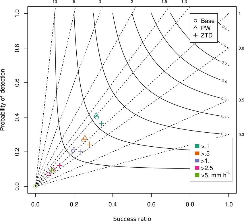
348 W. Rohm et al.: 4DVAR assimilation of GNSS zenith path delays
Table 1. The WRF configuration used in the experiment.
Parameters Domain 1 Domain 2
Spatial resolution 12 km × 12 km 4 km × 4 km
Vertical levels 48 48
Microphysics Thompson (Thompson et al., 2004) Thompson (Thompson et al., 2004)
Cumulus Kain–Fritsch (Kain, 2004) –
Longwave radiation RRTM (Mlawer et al., 1997) RRTM (Mlawer et al., 1997)
Shortwave radiation Dudhia (Dudhia, 1989) Dudhia (Dudhia, 1989)
Surface layer MM5 (Paulson, 1970) MM5 (Paulson, 1970)
Planetary boundary layer Yonsei University scheme (Hong et al., 2006) Yonsei University scheme (Hong et al., 2006)
tion was run using a 4DVAR WRF DA system, only for in- cessing and quality monitoring of the data can be found in
ner domain (d02). Prediction model was started once a day, Bosy et al. (2012). Fifteen of the stations are a part of the
at 00:00 UTC. Assimilation window was centered around EUREF Permanent Network (EPN) and provide the tropo-
00:00 UTC. Background error covariance (BE) was selected spheric parameters with the accuracy required by NWP data
for regional application (cv_options = 5) (BE depends on the assimilation (Dymarska et al., 2017), i.e., the standard de-
WRF domain). BE was constructed based on a forecast for viation between GNSS ZTD and WRF ZTD is 10 mm and
convection events in the first week of May 2013. the standard deviation between radiosonde ZTD and WRF
Quality control was selected for SYNOP and RS data in ZTD is 14 mm. In the inter-comparison study using multi-
observation processor (obsproc) and in WRFDA. For ZTD ple techniques (Wilgan et al., 2015), the discrepancy between
and PW data, quality control was conducted before process- GNSS observations and radiosonde was found to be 10 mm.
ing, followed by obsproc verification and the last step in According to the EGVAP requirements (Offiler, 2012), this
4DVAR assimilation. The WRF configuration was based on accuracy of the GNSS data is sufficient for the assimilation
the best ensemble members (ens1) with a small modification in NWP models.
from ensemble system dedicated to Poland during summer-
time (Guzikowski et al., 2015). 2.3 Model evaluation
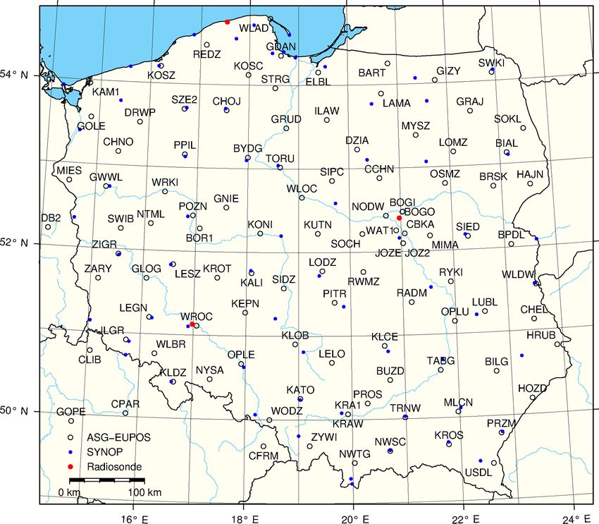
2.2 GNSS data The WRF model runs are compared with surface meteorolog-
ical measurements of air temperature, relative humidity, wind
The GNSS data are calculated by the GNSS and Meteo speed and precipitation, radiosonde temperature and relative
working group from the Institute of Geodesy and Geoinfor- humidity profiles in three locations across Poland, GNSS ob-
matics, Wrocław University of Environmental and Life Sci- servations in 106 locations.
ences (http://www.igig.up.wroc.pl/igg, last access: 17 Au- For the SYNOP, measurements are available every hour
gust 2018). The PW and ZTD values are calculated at 106 at 66 SYNOP stations, evenly distributed over the area of
stations of the European Position Determination System Ac- Poland, operated by the Institute of Meteorology and Wa-
tive Geodetic Network (ASG-EUPOS, http://www.asgeupos. ter Management – National Research Institute. Model eval-
pl, last access: 17 August 2018) in Poland and adjacent areas uation is performed only for the nested domain. Four error
(Fig. 2). metrics are calculated to assess the forecast performance.
The GNSS parameters are calculated from GPS data only,
using the Bernese GNSS Software version 5.0 (Dach et al., – Mean error (ME), which describes the model tendency
2007). The parameters (coordinates and troposphere) are es- of overestimation (ME > 0) or underestimation (ME < 0)
timated in a near-real time (NRT) regime, 30 min after each of the given meteorological parameter. The ME (bias)
full hour, without the gradient estimation. The dry tropo- is calculated as a mean difference between the modeled
sphere a priori model is taken from Saastamoinen (1972), and observed values for all stations (domain wide). The
mapped with dry Niell MF (Niell, 2000) and the ZTD rel- units are the same as for the analyzed meteorological
ative constraining of 3 mm is applied. International GNSS parameters.
Service (IGS) ultra-rapid orbits, clocks and Earth rotation
parameters are used. These parameters are now altered to fit
the more recent version of Bernese (5.2) (Dach et al., 2015; – Root mean square error (RMSE), which takes only non-
Dymarska et al., 2017), but this study uses NRT data, orig- negative values. The RMSE (scatter) is calculated as a
inally processed in 2013. In this way, our impact study will root of the squared differences between the modeled and
show the minimum potential of GNSS data assimilation in observed values for all stations. The units are the same
weather model exactly. More details on the GNSS data pro- as for the analyzed meteorological parameters.
Atmos. Meas. Tech., 12, 345–361, 2019 www.atmos-meas-tech.net/12/345/2019/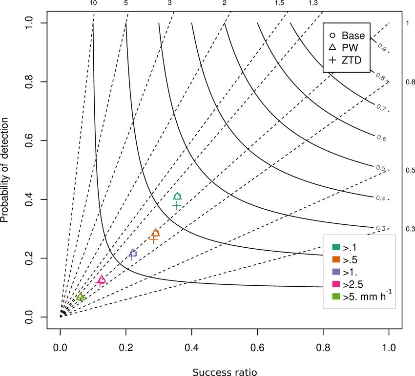
W. Rohm et al.: 4DVAR assimilation of GNSS zenith path delays                                                                          349

Figure 2. Location of the GNSS, SYNOP and radiosonde stations in Poland.

  – Pearson correlation coefficient (corr), which takes val-        and June case (large data set) we provide (Fig. 4) profile
    ues from −1 to +1, and the expected value is 1. Corr is         mean error with standard deviation multiplied by 1.96 (p =
    unitless.                                                       0.05), for other cases (much fewer observations) only mean
                                                                    errors are provided (Figs. 6, 10, 12). A similar comparison
  – Index of agreement (IOA), developed by Willmott                 was done by Guerova et al. (2005). The model based PW
    (1981) as a standardized measure of the degree of model         and ZTD are also compared to the GNSS based retrievals.
    prediction error. IOA varies between 0 and 1, and 1 in-         Bias and standard deviation of the residual WRF based PW
    dicates a perfect match.                                        and ZTD minus GNSS observed PW and ZTD are calculated
Model performance verification is done using observations           for 106 stations.
for rainfall, wind speed, relative humidity and air tempera-
ture at 2 m. The model evaluation is done for each simulation
considering the entire period and for different lead times and      3      Methodology
for selected days during which severe weather was observed
                                                                    The variational assimilation is based on the Bayesian proba-
(case studies). For rainfall forecasts, binary evaluation is also
                                                                    bility theory and it states that the model analysis is inferred
presented using performance diagrams (Roebber, 2009), sep-
                                                                    from two probabilities: background and observations. These
arately for five different precipitation intensity thresholds.
                                                                    can also be expressed as a minimization of a cost function,
The closer data set is towards the upper-right corner of the
                                                                    with two major components: background B and observations
plot the better performance of the forecasts.
                                                                    R error covariance (Ide et al., 1997; Lorenc, 1986; De Pon-
   Additionally, the model performance for air temperature
                                                                    deca and Zou, 2001) in the 4DVAR implementation:
and relative humidity was compared with radiosonde data,
available with a high vertical resolution for three stations lo-                    1h                    iT   h                   i
cated in Poland: Łeba, Warsaw and Wrocław, For the May              J [x (to )] =      x (to ) − x b (to ) B0−1 x (to ) − x b (to )
                                                                                    2

www.atmos-meas-tech.net/12/345/2019/                                                        Atmos. Meas. Tech., 12, 345–361, 2019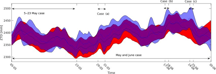
350                                                           W. Rohm et al.: 4DVAR assimilation of GNSS zenith path delays

       1 Xn
              Hi [x (ti )] − yio Ri−1 Hi [x (ti )] − yio ,           3.2   GNSS data preprocessing

   +      i=0
                                                              (1)
       2
where x (ti ), x b , x (to ), are model state vectors at the time    Two kinds of GNSS data are accepted by WRFDA package:
ti , and background vector and model initial conditions t0 ,         ZTD and PW. In order to prepare the GNSS estimates for
respectively. In general cases, there are N kinds of obser-          GPSPW, a preprocessing is required. The ZTD data are pro-
vations y defined at discrete times ti from to to tn , where         cessed according to the following steps.
the assimilation window spans from the lowest to the high-            1. Calculation of the GNSS ZTD using Bernese software
est ti . The Hi [x (ti )] is a forward operator that transforms          for all the stations.
parameters from the model space to the observation space.
The 3DVAR differs to 4DVAR by taking ti equal to obser-               2. Assimilation of the GNSS ZTD obtained in step (1) us-
vation time and analysis time. Minimization of the Eq. (1)               ing the 3DVAR scheme.
requires also finding adjoint (ADJ) and tangent linear (TLM)          3. Calculation of average ‘background’ corrections from
operators, each related to the observation type and forward              the WRF model for each station to reduce the system-
operator Hi [x (ti )]. For more details, the readers are referred        atic error between WRF and GNSS data and subtract-
to, e.g., Barker et al. (2004) or Huang et al. (2009).                   ing the corrections from the GNSS ZTD obtained in the
                                                                         step (1).
3.1    GPSPW operator
                                                                     In the first step, we adjust the formal errors of GNSS ZTD by
The WRFDA system employed in this study hosts varia-                 multiplying them by a factor of 10.5 mm, in which is the stan-
tional (VAR) 3D/4D as well as hybrid variational ensemble            dard deviation of differences between WRF ZTD and GNSS
algorithms (Barker et al., 2012). Currently, the system sup-         ZTD according to Dymarska et al. (2017). Next, we remove
ports the assimilation of surface, radiosonde, aircraft, wind        the observations, which errors exceed 20 mm, which is the
profile observations, as well as atmospheric motion vec-             standard procedure in GNSS data assimilation (Bennitt and
tors, radar reflectivities, spectrometric, GPS radio occulta-        Jupp, 2012).
tion and GPS ground-based data. The latter is linked di-                In the second step, the GNSS data are assimilated in the
rectly to the GPSPW operator (the National Center for At-            3DVAR procedure in order to calculate the corrections that
mospheric Research and WRF Model Users’ Page, 2017).                 come from the “background”, which is the WRF model. The
The operator defines the forward, tangent linear and adjoint         corrections for each day are expressed as O − B, where O is
of H for the 4DVAR and 3DVAR case for both ZTD and                   the “observation” ZTD (in this case same as ZTDGNSS from
PW. The operator also defines the observation covariance             the first step), and B is “background” ZTD, i.e., the WRF
R; in here diagonal matrix is assumed, with no correlation           ZTD. The corrections are then averaged over the entire con-
between observations, which requires spatial and temporal            sidered period to obtain one value (O − B)av for each station.
thinning (Bennitt et al., 2017; Bennitt and Jupp, 2012). The            In the third step, the corrected ZTDs are calculated as fol-
ZTD forward operator H reads as follows (Vedel and Huang,            lows:
2004) with further corrections made by Yong-Run Guo (from
da_transform_xtoztd module of GPSPW):                                ZTDcorr = ZTDGNSS − (O − B)av .                            (4)
                                Xk=kte  wdk1 p(i, j, k)q(i, j, k)   The PW data are processed in a similar way.
ZTD (i, j ) = ZHD (i, j ) +         k=kts         t (i, j, k)         1. Calculation of the GNSS PW from GNSS data.

              wdk3 p(i, j, k)q(i, j, k) 1h
            +                                   ,             (2)     2. Assimilation of the GNSS PW obtained in the step
                      t 2 (i, j, k)         aew                          (1) using the 3DVAR scheme.
where ij k are indices of model nodes, p is a pressure, q is
                                                                      3. Calculation of “background’‘ corrections and subtract-
specific humidity, t is temperature, 1h is a height difference
                                                                         ing them from the GNSS PW obtained in the step (1).
between two consecutive model layers, aew = 0.622 is a con-
stant, wdk1 = 2.2110−7 , wdk3 = 3.73 10−3 are compress-              From GNSS processing, we can only estimate ZTDs. The
ibility constants, ZHD is a zenith hydrostatic delay computed        PWs in step (1) are calculated in a standard way from GNSS
according to the (Saastamoinen, 1972) explicitly given in            and WRF data as follows:
Eq. (6).
                                                                     PW = Q · (ZT DGNSS − ZHDWRF ),                             (5)
   The PW forward operator is formed similarly to the ZTD
operator (following da_integrat_dz module of GPSPW oper-             where ZHDWRF is the hydrostatic delay calculated using
ator):                                                               Saastamoinen (1972) formula from pressure from WRF
             Xk=kte                                                  model pWRF , height h and latitude ϕ of a GNSS station:
PW (i, j ) =     k=kts
                       (ρ(i, j, k)q(i, j, k)1h) ,          (3)
                                                                                            0.0022767pWRF
where ρ is air density.                                              ZHDWRF =                                         .         (6)
                                                                                  1 − 0.00266 cos (2ϕ) − 0.00000029 h

Atmos. Meas. Tech., 12, 345–361, 2019                                                   www.atmos-meas-tech.net/12/345/2019/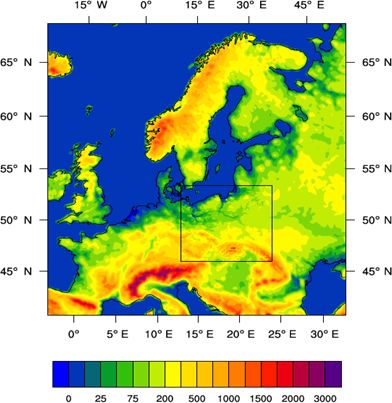
W. Rohm et al.: 4DVAR assimilation of GNSS zenith path delays                                                                351

The proportionality factor Q is calculated as follows:               The first severe weather case study (case a) was observed
                                                                  in 29–31 May 2013. The weather event is related to an un-
            106                                                   usual, low-pressure regions: (1) that developed over Hungary
Q=                                                         (7)
     Rw (k3 /Tm + k2 0 )                                          and moving towards Czechia, and (2) that developed over
                                                                  Moldova and moving towards the east of Poland. In these
where Rw = 461.525 [J (K kg)−1 ] is the gas constant of a wet     two lows, in the presence of stratified clouds, the cumulonim-
air, k2 0 = 22.9726 [K hPa−1 ] and k3 = 375463 [K2 hPa−1 ]        bus clouds develop and form a supercell. It brought intensive
are the “best average” refractivity constants from Rueger         rain and hail, however the precise location of such supercells
(2002) and Tm is the mean temperature calculated from TWRF        is not easy to predict (http://www.meteo.pl, last access: 17
as follows:                                                       August 2018).
                                                                     The second analyzed case (case b) occurred in 17–
Tm = 70.2 + 0.72 · TWRF .                                  (8)    18 June 2013 and is related to two weather systems: (1) high
                                                                  pressure system with a center in Belarus affecting northern
After calculation of GNSS PW, the processing in steps (2)
                                                                  part of Poland, (2) low pressure system over the Bay of Bis-
end (3) is analogical to GNSS ZTD.
                                                                  cay. Cold weather is observed in the north (20 ◦ C) and hot
                                                                  and humid in the south (above 30 ◦ C). The thermic contrasts
4   Case studies                                                  and warm unstable air result in the occurrence of convective
                                                                  cells located southeast of the region. These cells merged in
All cases presented in this study are selected from the period    the late afternoon and formed a supercell storm that moved
of May–June 2013 in Central Europe covering the bench-            southward to the Moravia region (http://www.meteo.pl).
mark campaign of COST Action ES1206 (Douša et al.,                   The third case analyzed was 24–25 June 2013. The
2016). The following experiments are considered (Fig. 3):         weather in Europe was driven by high pressure system lo-
(1) assimilation of ZTD or PW for all of May and June 2013,       cated over the Atlantic Ocean, as well as large and shallow
(2) assimilation of ZTD or PW and ZTD or PW with sup-             trough extending north to Norway from a weak low centered
port of RS and SYNOP for 5–23 May 2013, (3) case stud-            over the northern part of the Adriatic Sea (with the atmo-
ies a, b and c, showing impact of assimilation of ZTD or          spheric pressure of around 1010 hPa). Secondary cyclogene-
PW in severe weather cases which took place during May            sis is organized over central Poland in the form of a thermal
and June 2013. The mean and standard deviation of ZTD             asymmetric low pressure system. A quasi-stationary anabatic
from GNSS and from WRF are presented in the Fig. 3. The           cold front spread along this trough changing its position very
overall agreement between GNSS and WRF traces are high;           slowly and bringing cold air from the north (in the western
however, the WRF model is negatively biased with respect to       part of Poland), and warm, humid and unstable air masses
the observations and shows fewer variations. Moreover, few        from the south (in the eastern part of Poland). These condi-
cases of significant departure of WRF ZTD from GNSS ZTD           tions are prone to developing strong precipitation, thunder-
are visible in June, two are collocated with case b and case c    storms and hail in central Poland (http://www.meteo.pl).
investigated in this study.
   According to synoptic analysis presented in Douša et           4.1     Assimilation of GNSS observations
al. (2016), the beginning of May 2013 was characterized by
a cyclonic field over 500 hPa, which in turn resulted in pre-     The full period of 2 months is used as a first approach to
cipitation and convection development, moving from west to        validate the impact of PW or ZTD data on weather forecasts
east. The mid-May weather in the region was developing un-        using radiosonde, GNSS and SYNOP observations.
der the influence of an upper-level cyclone (500 hPa) that
brought the cold advection from west. Towards the end of          4.1.1    Comparison to radiosonde profiles
May, a series of Atlantic cyclones approached Europe. The
end of the month brought a stop to the advection of cold air      It is expected that the ZTD and PW assimilation first will af-
by the upper-east ridge, which pushed the cyclones more to        fect the 3D distribution of humidity and temperature. This is
the south and brought humid and warm air to Central Europe.       summarized in Fig. 4. and Table 2. In the case of relative hu-
In June, three flooding events were recorded in the Czech Re-     midity, assimilation of ZTD significantly improves the model
public, which were associated with baroclinic instability de-     performance in the layer from 2.5 to 10 km, with a 22 % im-
veloping over the area of interest, with a first one (1–3 June)   provement over the base simulation. At the same time, this
event unexpected and of disastrous nature while two latter        assimilation increases the model error for air temperature,
(9–11; 23–26 June) less severe and better predicted. As in        but only in the range 2.5–5.0 km and above 10 km. Assim-
this work, we use Poland as a study region, there is a time       ilation of PW has a small impact on both relative humidity
shift between the events recorded in Czech Republic (de-          and air temperature, and the errors, both in terms of the value
scribed by Douša et al., 2016) and Poland and also the pre-       and vertical distribution is very similar if PW and base runs
cipitation effects were not as disastrous.                        are compared (Fig. 4 and Table 2). The assimilation of PW

www.atmos-meas-tech.net/12/345/2019/                                                  Atmos. Meas. Tech., 12, 345–361, 2019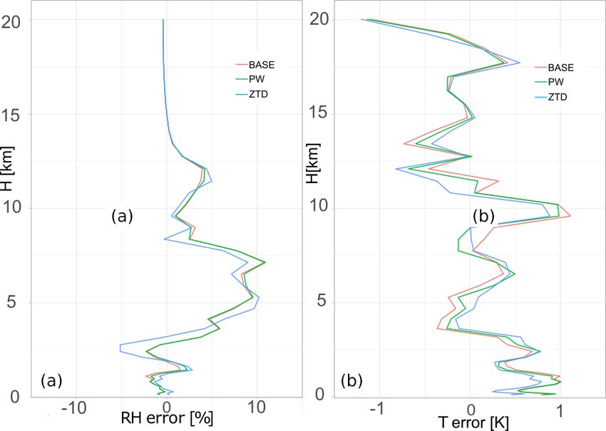
352                                                           W. Rohm et al.: 4DVAR assimilation of GNSS zenith path delays

Figure 3. Time evolution of mean ZTD in the study domain for WRF (red) and GNSS (blue) data (solid lines). Filled area marks standard
deviation spread around mean values. Arrows represent the time and duration of analyzed cases.

                                                                     Table 2. Mean error for RH and T calculated for selected height
                                                                     classes for May and June 2013. Lead time is 12 h. Font denotes
                                                                     improvement (bold), deterioration (bold/italic) or no impact (italic)
                                                                     on the forecast with the use of GNSS data.

                                                                                       RH mean error [%]              T mean error [K]
                                                                       Height          Base    PW     ZTD        Base         PW    ZTD
                                                                       < 2.5 km        3.35    3.47    3.85      0.25       0.26     0.19
                                                                       2.5–5.0 km      2.26    2.74    2.01      0.04       0.06     0.14
                                                                       5.0–10.0 km     7.55    7.71    5.94     −0.03      −0.02     0.02
                                                                       > 10.0 km       2.32    2.25    2.14      0.00       0.00     0.04

                                                                     Table 3. Bias and standard deviation for PW and ZTD calculated
                                                                     for all GNSS stations in the experiment for May and June 2013.
                                                                     Lead time < 24 h. Font denotes improvement (bold), deterioration
                                                                     (bold/italic) or no impact (italic) on the forecast with the use of
                                                                     GNSS data.
Figure 4. Vertical distribution of mean error for base, PW and ZTD
                                                                                Parameter     Run     Bias [mm]         std [mm]
for May and June 2013 for relative humidity (a) and air tempera-
ture (b). The errors are calculated for the lead time 12 h.                     PW            Base              2.6           4.9
                                                                                              PW                2.5           4.7
                                                                                              ZTD               2.6           4.7
result in significant increase of errors (by 20 %), only in the                 ZTD           Base            −8.3           26.5
2.5–5.0 km section of troposphere.                                                            PW              − 8.8          25.7
                                                                                              ZTD             −8.1           26.0
4.1.2   Comparison to GNSS observations

The assimilation of the GNSS products should also have               comparison (not shown) produces similar results across all
an impact on the PW and ZTD estimates from the WRF                   stations, hence mean statistics is calculated (Table 3).
model. We compare the PW and ZTDs calculated from WRF                   In general, the assimilation of the GNSS does not bring a
using formulas (2) and (3) respectively using NCAR com-              huge improvement in the WRF estimates. For PW, the bias,
mand language (NCL) (NCAR, 2018), before the assimi-                 averaged from all stations equals to 2.6 mm for the base run,
lation (“base”) and after the assimilation of both PW and            and is slightly improved by 0.1 mm the PW assimilation and
ZTDs. The comparisons are performed for the GNSS data                remains same for ZTD assimilation. The average standard
before the processing described in Sect. 3.1. Thus, the pre-         deviations for the estimates after assimilation improves by
sented biases for the base run are removed from the GNSS             0.2 mm for both PW and ZTDs. For the ZTD assimilation,
to better fit the observations to the model. Station by station      there is degradation of the ZTD biases after the assimilation

Atmos. Meas. Tech., 12, 345–361, 2019                                                     www.atmos-meas-tech.net/12/345/2019/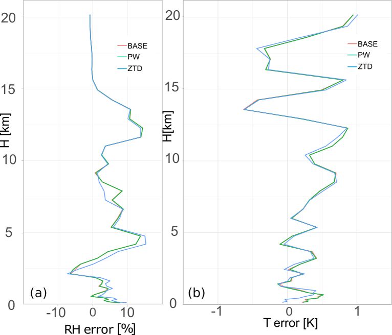
W. Rohm et al.: 4DVAR assimilation of GNSS zenith path delays                                                                       353

of PW (by 0.5 mm) but also improvement in the case of ZTD
assimilation (by 0.2 mm). The assimilation of both PW and
ZTD brings an improvement of the ZTD standard deviations
for almost all of the stations, therefore the average standard
deviations decrease for both PW and ZTD assimilation.

4.1.3   Comparison to SYNOP

Further forecast verification is based on 66 SYNOP stations
distributed evenly across Poland (Fig. 2). Table 4 summarizes
model forecast performance using ME, RMSE, corr and IOA.
The statistics are calculated for lead times from 1 to 24 h for
the following parameters: rain intensity (rain), wind speed
(wspd), relative humidity (rh2) and temperature (T 2).
   The overall accuracy of the rain forecast is low, i.e., the
base run prediction correlates with the observations in less
than 15 %, while the same parameter for wind speed is close
to 60 %, whereas corr for relative humidity is 82 % and for
temperature 95 %. As the assimilation changes the initial
conditions of parameters directly linked with the adjoint op-
                                                                       Figure 5. Performance diagram for assimilation of ZTD and PW for
erator (a transpose of forward operator), the impact while us-
                                                                       May and June 2013 (lead time < 24 h). The various colors represent
ing ZTD should be visible in pressure p (Eq. 2) (and thus also         rain intensity classes, whereas the shapes represent data sets.
wind speed), specific humidity q (and thus relative humidity)
and temperature t. Whereas PW should have impact mostly
on specific humidity q (Eq. 3) and thus on the rh2 parameter.          4.2     Assimilation of GNSS, RS and SYNOP
Rain as a parameter linked with physical parameterization                      observations
and many other variables such as humidity, vertical and hori-
zontal motion, or temperature profile are also sensitive to the        In the second experiment, we focus on a short time span cov-
GNSS data assimilation.                                                ering May with moderate precipitation and standard cyclonic
   The results (Table 4) confirm that the assimilation of PW           weather, as opposed to June, with the occurrence of major se-
over the whole period of 2 months affects the forecasts only           vere weather events (analyzed in Sect. 4.3). This experiment
slightly, the assimilation increases the relative humidity scat-       is prepared to assess the impact of using RS and SYNOP to-
ter and has negative or neutral impact on the rain ME and              gether with GNSS data in 4DVAR assimilation.
RMSE, neutral or positive impact on wind speed and nega-
tive or neutral impact on temperature. Similarly, there is no          4.2.1    Comparison to radiosonde profiles
gain for rainfall forecasts if ZTD is assimilated for the entire
period. It has a negative impact on wind speed, but there are          Comparison to radiosonde data (Fig. 6, Table 5) shows that
considerable improvements for the relative humidity forecast           largest impact on RH is visible in relatively high levels of
(15 % reduction of ME).                                                troposphere 7–10 km, however improvements to this param-
   The negative impact of ZTD on the wind speed forecast               eter are also present for 2.5–5.0 km range. Assimilation of
could be linked to the representation of ZHD as a parame-              PW+SYNOP+RS result in highest gain of quality (in the
ter related only to ground-based observations of temperature           section 5–10 km by 10 %). In the lower part this impact is
and pressure (Eq. 2), whereas in reality the ZHD is an in-             less visible (for any observation type), however below 2.5 km
tegral of pressure and temperature across the whole tropo-             assimilation of PW and ZTD alone increase ME (8 % for PW
sphere (Vedel and Huang, 2004).                                        and 2 % for ZTD). The impact on temperature is noted only
   If the rainfall forecasts are analyzed more closely using the       in the 12.5–15 km sector. Use of SYNOP and RS data im-
binary verification with data stratification according to rain-        proves forecast in all cases but largest increase is visible in
fall intensity (Fig. 5), it is clear that the PW run is very similar   the PW observations and in the 2.5–10 km section.
to the base run, regardless of the rainfall intensity. The ZTD
                                                                       4.2.2    Comparison to GNSS observations
assimilation leads to an overall decrease of the probability of
detection.                                                             Comparing all active GNSS stations ZTDs and PWs to the
                                                                       WRF based ZTDs and PWs (Table 6), one notice no im-
                                                                       pact on the PW for ZTD and PW assimilation (both bias
                                                                       and std), whereas for the same experiments ZTD bias in-
                                                                       creased but scatter decreased considerably (reduction of std

www.atmos-meas-tech.net/12/345/2019/                                                        Atmos. Meas. Tech., 12, 345–361, 2019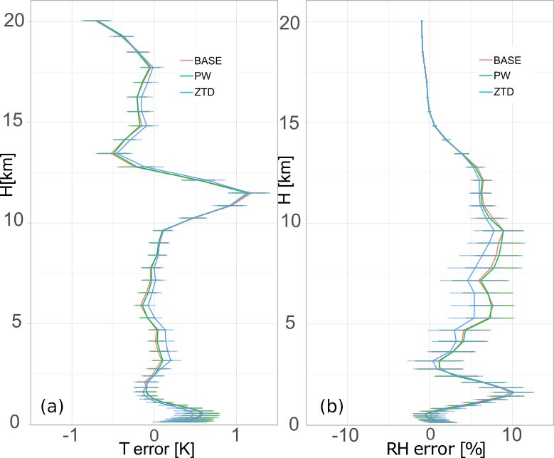
354                                                                            W. Rohm et al.: 4DVAR assimilation of GNSS zenith path delays

Table 4. Impact of assimilation of PW and ZTD using 4DVAR operators, validated against SYNOP observations for June and May (lead
time < 24 h). Font denotes improvement (bold), deterioration (bold/italic) or no impact (italic) on the forecast with the use of GNSS data.

 Run                                    rain                              wspd                                       rh2                                     T2
                            me    RMSE          corr    IOA      me    RMSE      corr      IOA          me    RMSE           corr    IOA       me     RMSE         corr    IOA
 Base May and June    −0.680       2.567       0.123   0.380   0.055   1.522    0.589   0.760     −2.098      10.643       0.823    0.903   −0.351     2.244      0.918   0.956
 PW                   −0.684       2.559       0.124   0.381   0.057   1.520    0.590   0.760     −2.104      10.658       0.822    0.902   −0.352     2.246      0.918   0.956
 ZTD                  −0.720       2.570       0.122   0.380   0.083   1.526    0.584   0.756     −1.765      10.577       0.823    0.904   −0.409     2.243      0.919   0.956

Table 5. Mean error for RH and T calculated for selected height classes for 5–23 May 2013. Lead time is 12 h. Font denotes improvement
(bold), deterioration (bold/italic) or no impact (italic) on the forecast with the use of GNSS data.

                                               RH mean error [%]                                                             T mean error [K]
  Height             Base        PW        PW+SYNOP            ZTD     ZTD+SYNOP                 Base          PW          PW+SYNOP            ZTD       ZTD+SYNOP
                                                +RS                          +RS                                                +RS                            +RS
  < 2.5 km           5.05        5.49                  5.19    5.19                 5.18     −0.04           −0.12                  −0.10    −0.15                   −0.15
  2.5–5.0 km         3.16        3.31                  2.92    2.99                 3.06     −0.04           −0.04                  −0.05    −0.02                   −0.02
  5.0–10.0 km        6.47        6.43                  5.72    6.05                 6.35     −0.07           −0.08                  −0.10    −0.07                   −0.06
  > 10.0 km          2.15        2.05                  2.01    2.04                 2.03      0.01            0.02                   0.03     0.02                    0.02

                                                                                        Table 6. Bias and standard deviation for PW and ZTD calculated for
                                                                                        all GNSS stations in the experiment for 5–23 May 2013. Lead time
                                                                                        < 24 h. Font denotes improvement (bold), deterioration (bold/italic)
                                                                                        or no impact (italic) on the forecast with the use of GNSS data.

                                                                                                   parameter           run                            bias          std
                                                                                                                                                     [mm]         [mm]
                                                                                                   PW                  Base                            6.3          5.2
                                                                                                                       PW                              6.3          5.2
                                                                                                                       ZTD                             6.3          5.3
                                                                                                                       PW+SYNOP+RS                     6.3          5.2
                                                                                                                       ZTD+SYNOP+RS                    6.3          5.2
                                                                                                   ZTD                 Base                          −2.0          25.1
Figure 6. Vertical distribution of mean error for the base, PW,                                                        PW                            − 2.9         23.9
PW+SYNOP+RS, ZTD and ZTD+SYNOP+RS for 5–23 May for                                                                     ZTD                           − 2.8         23.9
relative humidity (a) and air temperature (b). The errors are calcu-                                                   PW+SYNOP+RS                   − 2.1         24.6
lated for the lead time 12 h.                                                                                          ZTD+SYNOP+RS                  − 2.4         24.6

by 1.2 mm). The combination of PW+SYNOP+RS and
ZTD+SYNOP+RS if PW field is considered no different to
the base run, whereas in the case of ZTD being used as a                                4.2.3      Comparison to SYNOP
diagnostic variable, the PW+SYNOP+RS provides best so-
lution from all assimilation cases, in terms of bias (only by                           The MEs for base run forecasts in May (Table 7) are lower
0.1 mm). Also mean station deviation is lower for assimilated                           than for May and June, e.g., rain ME is approx. −0.5 whereas
cases than for base simulation.                                                         May and June is approx. −0.7, May relative humidity ME
                                                                                        is approx. 0.4 % and May and June is approx. −2.1 %. Wind
                                                                                        speed errors are similar or slightly higher in May than in May
                                                                                        and June. A similar statement is correct for temperature er-
                                                                                        rors. The overall correlation between observations and fore-
                                                                                        casts is in the range from 13 % to over 17 % for rain, 56 % for
                                                                                        wspd, 82 % for rh2 and 91 % for T 2, which is a few percent
                                                                                        lower than in the May and June run (except for rain).

Atmos. Meas. Tech., 12, 345–361, 2019                                                                                 www.atmos-meas-tech.net/12/345/2019/
W. Rohm et al.: 4DVAR assimilation of GNSS zenith path delays 355
Table 7. Impact of assimilation of PW, ZTD, RS and SYNOP using 4DVAR operators, validated against SYNOP observations, for 5–
23 May 2013 (lead time < 24 h). Font denotes improvement (bold), deterioration (bold/italic) or no impact (italic) on the forecast with the
use of GNSS data.
Rain wspd rh2 T2
Run me RMSE corr IOA me RMSE corr IOA me RMSE corr IOA me RMSE corr IOA
Base May −0.475 2.027 0.132 0.383 0.046 1.551 0.565 0.742 0.352 10.987 0.819 0.903 −0.668 2.333 0.914 0.952
PW −0.509 1.933 0.171 0.419 0.080 1.563 0.557 0.737 0.771 10.855 0.825 0.906 −0.743 2.332 0.916 0.952
ZTD −0.543 1.903 0.166 0.417 0.082 1.554 0.559 0.738 0.729 10.938 0.822 0.904 −0.734 2.343 0.915 0.951
PW+ SYNOP+RS −0.494 1.990 0.150 0.401 0.043 1.556 0.554 0.735 0.697 10.875 0.824 0.906 −0.749 2.336 0.916 0.952
ZTD+SYNOP+RS −0.528 1.939 0.159 0.413 0.079 1.558 0.557 0.737 0.717 10.940 0.822 0.904 −0.751 2.336 0.916 0.952
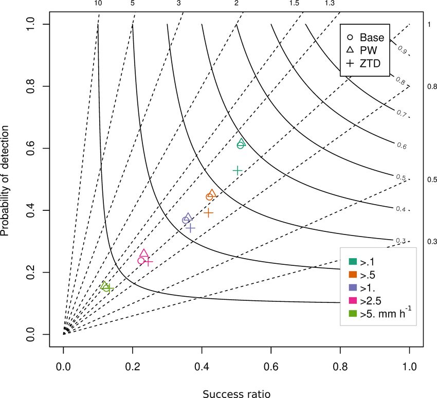
Table 7 shows comparison to SYNOP stations and it con- Binary rain analysis shows that the impact of data assim-
firms that the assimilation of either PW or ZTD has a nega- ilation on rainfall forecasts changes with rainfall intensity
tive impact on rain forecast in terms of mean error, however (Fig. 9). For the rainfall intensity above 0.1 mm h−1 , there
positive on all other statistics. The largest improvements are are small improvements for all the model runs if compared
for relative humidity, where all the statistics, except the ME, to the base run in terms of success ratio, but the probability
are improved if compared to base. Surprisingly, adding more of detection is smaller. The positive impact of data assimila-
observations, i.e., SYNOP and RS data, does not improve tion is much stronger for higher rainfall intensities. For the
rain or relative humidity forecast in the case of ZTD assimila- thresholds exceeding 1.0 mm h−1 , both probability of detec-
tion, but rather decreases the forecast’s quality. Assimilation tion and success ratio are improved if compared to the base
of both PW and ZTD deteriorates the model performance for run. The improvement is especially large for PW data assim-
wind speed. There is small but positive impact on the T 2 ilation and threshold > 5.0 mm h−1 .
forecast in terms of correlation coefficient, but, similarly to
RH, mean errors are increased if compared to base run. 4.3 Severe weather cases
As two forecasted parameters are improved, that is rel-
ative humidity and rain (see Table 7), we investigate the The final test is performed using selected three cases with
lead time differences between the base run and four as- strong instabilities and supercell storms. The overall impact
similation setups: namely PW, PW+SYNOP+RS, ZTD, of GNSS data in all cases is similar: if there is any reduction
ZTD+SYNOP+RS (Fig. 9). in uncertainty it is visible mostly in the rain and relative hu-
The Fig. 7 ME (left panel) of rain forecast varies signifi- midity forecast, with a small negative or neutral impact on
cantly over 24 h, especially in the lead time 10 to 24 h and is the wind speed and temperature forecasts.
relatively stable between 1 to 9 h (nighttime). In the scattered
section of Fig. 9, the ZTD+SYNOP+RS solution seems pos- 4.3.1 Case (a) 29–31 May 2013
itive most of the time, while it is negative in the first 9 h of
forecast. In the first 9 h of the forecast PW+SYNOP+RS re- The comparison of WRF-based RH and T with radiosonde
duces the forecast bias. PW and ZTD alone are rarely ob- shows that for case (a) (Fig. 10) the impact of ZTD assimi-
served to improve ME of rain forecast. The RMSE pictured lation introduces large change into the initial conditions and
on the right panel of Fig. 7 shows, similar to ME, scat- forecast. This impact is RH positive in the first 2 km and be-
tered and compacted sections, however there is clear pos- tween 6 and 10 km and might be negative close to 2.5 km.
itive impact of assimilating GNSS observations, especially Temperature show mixed results, with stronger influence of
ZTD+SYNOP+RS in the short run (until 24 h). Overall, the ZTD and weaker for PW, but across the whole profile this im-
RS and SYNOP data helps to improve RMSE of rain fore- pact is small but positive. Moreover ZTD increase agreement
cast. between model and RS in the bottom 2 km of temperature
Less variation between the four scenarios is observed for profile.
relative humidity errors (Fig. 8). Both ME and RMSE are re- Comparing the forecast with assimilation of ZTD and PW
duced while assimilating each data type, with an exception with GNSS observations (Table 8), shows that both data re-
of lead time 15 h, when RMSE increases (more when ZTD duce scatter of the observations but ZTD is also reducing sys-
is used, less when PW is used). Moreover, the highest reduc- tematic effects, while PW is increasing bias.
tion of ME is noticed between 12 and 18 h of lead time for According to Table 9, which presents a comparison to
PW+SYNOP+RS scenario, but other scenarios also shows a SYNOP data, mixed results are observed for case (a). The
positive impact. It is also worth mentioning that the rh2 fore- rain forecast shows better performance if PW is compared
cast RMSE is reduced after 12 h lead time whereas bias is to base run. Assimilation of ZTD for this case deteriorates
constantly reduced starting from the first hour of forecast. model performance except for mean error. Humidity forecast
(rh2) is improved, in terms of RMSE and corr, when ZTD
www.atmos-meas-tech.net/12/345/2019/ Atmos. Meas. Tech., 12, 345–361, 2019356 W. Rohm et al.: 4DVAR assimilation of GNSS zenith path delays
Figure 7. Performance of rain intensity forecast with respect to lead time (positive – improvement with respect to the base run, negative –
deterioration with respect to the base run): (a) ME, (b) RMSE.
Figure 8. Performance of rh2 forecast with respect to lead time: (a) ME, (b) RMSE.
is assimilated. For PW assimilation, model performance is rainfall, except for ME reduction. The model performance
worse if compared to base. for other parameters is similar or slightly worse than base.
Binary analysis depicted in Fig. 11 shows the posi- ZTD assimilation has small positive impact on RMSE, corr
tive impact of assimilating of PW in a rainfall rate above and IOA of rain intensity forecast, but negative on ME. Rela-
0.5 mm h−1 , and ZTD above 2.5 mm h−1 . tive humidity ME is reduced by assimilation of ZTD by 43 %,
all other measures are better for base run. In the local type of
4.3.2 Case (b) 17–18 June 2013 rain in southeastern Poland, as in this case, it is impossible to
present statistically sound results for 5 rainfall classes, hence
The comparison of WRF-based RH and T with radiosonde we did not provide binary rain analysis for this case.
shows that for case (b) (Fig. 12) the impact of ZTD assim-
ilation introduces large change to the initial conditions and
forecast, while PW has almost no impact. The ZTD impact is 4.3.3 Case (c) 24–25 June 2013
negative in RH in the first 5 km and positive from 7 to 10 km.
The temperature profile shows positive results, with stronger The comparison of WRF-based RH and T with radiosonde
influence of ZTD and almost none for PW. It is visibly posi- shows that for case (c) (Fig. 13) the impact of ZTD assim-
tive in the bottom part of the troposphere (first 1 km). ilation introduces large change to the initial conditions and
Comparing forecast with assimilation of ZTD and PW consequently to the forecast. This impact is RH positive in
with GNSS observations (Table 8), shows that both data re- the first 1 km, negative close to 2.5 km and clearly positive at
duce the scatter of the observations. The bias for PW param- 5 km. Temperature shows mixed results, however it is worth
eter slightly increases for both types of assimilated observa- pointing out that from 2.5 to 5 km there is positive bias in-
tions, however ZTD bias is reduced. troduced to the forecast by both PW and ZTD. Temperature
Comparison to SYNOP data (Table 9) shows that, the as- is improved once ZTD is assimilated in the bottom part of
similation of PW does not change model performance for troposphere (first 1 km).
Atmos. Meas. Tech., 12, 345–361, 2019 www.atmos-meas-tech.net/12/345/2019/W. Rohm et al.: 4DVAR assimilation of GNSS zenith path delays 357
Table 8. Bias and standard deviation for PW and ZTD calculated for
all GNSS stations in the experiment for selected cases (case a) 29–
31 May 2013; (case b) 17–19 June 2013; (case c) 24–26 June 2013.
Lead time < 24 h. Font denotes improvement (bold), deterioration
(bold/italic) or no impact (italic) on the forecast with the use of
GNSS data.
Parameter Run Bias [mm] std [mm]
PW Base (case a) −0.6 2.9
PW (case a) −0.6 2.8
ZTD (case a) −0.4 2.7
Base (case b) −0.7 2.7
PW (case b) − 0.8 2.4
ZTD (case b) − 0.8 2.4
Base (case c) 0.4 3.4
PW (case c) 0.4 3.2
ZTD (case c) 0.5 3.2
ZTD Base (case a) −14.6 23.6
PW (case a) − 15.2 23.3
ZTD (case a) −14.2 23.3
Figure 9. Performance diagram for assimilation of PW, Base (case b) −11.0 22.0
PW+SYNOP+RS, ZTD+SYNOP+RS and ZTD for May 2013 PW (case b) −10.6 21.1
(lead time < 24 h). The various colors represent rain intensity ZTD (case b) −10.6 20.8
classes, whereas the shapes represent data sets. Base (case c) −34.9 23.9
PW (case c) −34.7 23.6
ZTD (case c) − 35.0 23.7
Figure 10. Vertical distribution of mean error for the base, PW, and
ZTD for case (a) in 29–31 May 2013 for relative humidity (a) and
air temperature (b). The errors are calculated for the lead time 12 h.
Comparing forecast with assimilation of ZTD and PW
with GNSS observations (Table 8), shows that both data re- Figure 11. Performance diagram for assimilation of PW and ZTD
duce scatter of the observations. The bias for PW parameters for case (a) (lead time < 24 h). The various colors represent rain
slightly increases (ZTD assimilation) or is neutral (PW as- intensity classes, whereas the shapes represent data sets.
similation). The bias for ZTD decreases for PW assimilation
and slightly increases for ZTD assimilation.
The third case, once compared to the SYNOP, also shows PW run, there is also a gain for relative humidity, while for
a small but positive impact of ZTD, especially in PW data as- ZTD error statistics are worse if compared to the base run.
similation on rainfall forecasts, except for mean error. Errors In the performance diagram in Fig. 14, the rain rate fore-
statistics are also improved for wind speed. In the case of the casts are improved with PW with respect to the base forecast,
www.atmos-meas-tech.net/12/345/2019/ Atmos. Meas. Tech., 12, 345–361, 2019358 W. Rohm et al.: 4DVAR assimilation of GNSS zenith path delays
Table 9. Impact of assimilation of PW, ZTD, RS and SYNOP using 4DVAR operators, validated against SYNOP observations, for selected
cases (case a) 29–31 May 2013; (case b) 17–19 June 2013; (case c) 24–26 June 2013 (lead time < 24h). Font denotes improvement (bold),
deterioration (bold/italic) or no impact (italic) on the forecast with the use of GNSS data.
rain wspd rh2 T2
Run me RMSE corr IOA me RMSE corr IOA me RMSE corr IOA me RMSE corr IOA
Base (case a) −1.233 3.412 0.020 0.327 0.416 1.870 0.569 0.722 −3.049 10.760 0.811 0.891 −0.102 2.506 0.862 0.923
PW (case a) −1.166 3.360 0.036 0.353 0.429 1.872 0.566 0.720 −3.130 10.807 0.810 0.891 −0.093 2.517 0.861 0.923
ZTD (case a) −1.155 3.609 −0.006 0.313 0.463 1.916 0.555 0.710 −2.774 10.623 0.811 0.893 −0.169 2.484 0.864 0.924
Base (case b) −2.016 4.626 −0.082 0.331 0.152 1.324 0.466 0.680 −0.597 10.197 0.826 0.907 −0.501 2.155 0.930 0.957
PW (case b) −2.012 4.626 -0.082 0.330 0.155 1.326 0.467 0.681 −0.566 10.244 0.824 0.906 −0.510 2.159 0.929 0.957
ZTD (case b) −2.026 4.625 −0.061 0.332 0.175 1.362 0.427 0.656 −0.092 10.286 0.823 0.906 −0.614 2.204 0.927 0.955
Base (case c) −0.701 3.240 0.223 0.490 −0.065 1.864 0.575 0.750 −4.444 10.970 0.760 0.842 −0.004 2.210 0.865 0.929
PW (case c) −0.739 3.135 0.250 0.510 −0.064 1.859 0.577 0.751 −4.455 10.913 0.764 0.843 −0.004 2.205 0.866 0.929
ZTD (case c) −0.803 3.167 0.250 0.508 −0.030 1.835 0.576 0.750 −4.433 11.066 0.760 0.841 −0.044 2.216 0.868 0.930
Figure 13. Vertical distribution of mean error for the base and PW
for case (c) 24–26 June, for relative humidity (a) and air tempera-
ture (b). The errors are calculated for the lead time 12 h.
Figure 12. Vertical distribution of mean error for the base, PW and
ZTD for case (b) 17–18 June, for relative humidity (a) and air tem- weather occurrence were investigated. All were linked to a
perature (b). The errors are calculated for the lead time 12 h. supercell development and intense rain.
The major conclusion of this study is that for the ana-
lyzed time period, with more than 100 stations involved in the
but worse when ZTD is assimilated. This effect is visible for experiment, there are two parameters significantly changed
all rain rates lower than 1 mm h−1 and this discrepancy disap- once GNSS data are assimilated in the WRF model using
pears for rain rates in the 2.5 mm h−1 class, where both ZTD GPSPW operator and these are the moisture field and rain.
and PW have positive impact, whereas no impact is noticed Other parameters such as pressure or temperature field are
for rainfall rates above 5 mm h−1 . not changed from initial conditions significantly. The GNSS
observations improves forecast in the first 24 h but with
strongest impact starting from 9 h lead time. It is worth notic-
5 Summary and conclusions ing that even moderate quality NRT estimates used in this
study (ZTD discrepancy ∼ 10–15 mm) are improving rela-
In this study, we have analyzed 2 months (May and tive humidity forecast, moreover the impact of ZTD is posi-
June 2013) of 4DVAR assimilation of GNSS ground-based tive in the vertical profile (over 20 % decrease of mean error)
observations in WRF model from over 100 stations in starting from 2.5 km upward. Even if the humidity forecast
Poland. Two major approaches were investigated using GP- in lower part of troposphere (below 2.5 km) after GNSS data
SPW operator: assimilation of PW and ZTD. For a shorter assimilation deteriorates, the SYNOP observations confirms
time period of 18 days in May additional data were assimi- that ZTD has positive impact on the rh2 parameter. Assim-
lated: namely RS and SYNOP observations across Poland. ilation of PW has less significant impact on both humidity
Moreover, three different case studies related to severe and rain forecasts in the vertical profile and on the ground,
Atmos. Meas. Tech., 12, 345–361, 2019 www.atmos-meas-tech.net/12/345/2019/You can also read