A 99-Day Assessment of the Weather Research and Forecasting Model over the Southwest United States - by John W Raby, Huaqing Cai, Leelinda Dawson ...
←
→
Page content transcription
If your browser does not render page correctly, please read the page content below
ARL-TR-9237 ● JULY 2021

A 99-Day Assessment of the Weather Research
and Forecasting Model over the Southwest
United States
by John W Raby, Huaqing Cai, Leelinda Dawson, and
Brian Reen

Approved for public release: distribution unlimited.
NOTICES

                                    Disclaimers

The findings in this report are not to be construed as an official Department of the
Army position unless so designated by other authorized documents.
Citation of manufacturer’s or trade names does not constitute an official
endorsement or approval of the use thereof.
Destroy this report when it is no longer needed. Do not return it to the originator.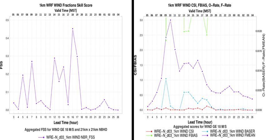
ARL-TR-9237 ● JULY 2021

A 99-Day Assessment of the Weather Research
and Forecasting Model over the Southwest
United States

John W Raby, Huaqing Cai, Leelinda Dawson, and Brian Reen
Computational and Information Sciences Directorate,
DEVCOM Army Research Laboratory

Approved for public release: distribution unlimited.
Form Approved
                                 REPORT DOCUMENTATION PAGE                                                                                                         OMB No. 0704-0188
Public reporting burden for this collection of information is estimated to average 1 hour per response, including the time for reviewing instructions, searching existing data sources, gathering and maintaining the
data needed, and completing and reviewing the collection information. Send comments regarding this burden estimate or any other aspect of this collection of information, including suggestions for reducing the
burden, to Department of Defense, Washington Headquarters Services, Directorate for Information Operations and Reports (0704-0188), 1215 Jefferson Davis Highway, Suite 1204, Arlington, VA 22202-4302.
Respondents should be aware that notwithstanding any other provision of law, no person shall be subject to any penalty for failing to comply with a collection of information if it does not display a currently
valid OMB control number.
PLEASE DO NOT RETURN YOUR FORM TO THE ABOVE ADDRESS.
1. REPORT DATE (DD-MM-YYYY)                             2. REPORT TYPE                                                                      3. DATES COVERED (From - To)
July 2021                                               Technical Report                                                                    01 October 2019–30 September 2020
4. TITLE AND SUBTITLE                                                                                                                       5a. CONTRACT NUMBER
A 99-Day Assessment of the Weather Research and Forecasting Model over the
Southwest United States                                                                                                                     5b. GRANT NUMBER

                                                                                                                                            5c. PROGRAM ELEMENT NUMBER

6. AUTHOR(S)                                                                                                                                5d. PROJECT NUMBER
John W Raby, Huaqing Cai, Leelinda Dawson, and Brian Reen
                                                                                                                                            5e. TASK NUMBER

                                                                                                                                            5f. WORK UNIT NUMBER

7. PERFORMING ORGANIZATION NAME(S) AND ADDRESS(ES)                                                                                          8. PERFORMING ORGANIZATION REPORT NUMBER
DEVCOM Army Research Laboratory
ATTN: FCDD-RLC-EM                                                                                                                           ARL-TR-9237
White Sands Missile Range, NM 88002
9. SPONSORING/MONITORING AGENCY NAME(S) AND ADDRESS(ES)                                                                                     10. SPONSOR/MONITOR'S ACRONYM(S)

                                                                                                                                            11. SPONSOR/MONITOR'S REPORT NUMBER(S)

12. DISTRIBUTION/AVAILABILITY STATEMENT
Approved for public release: distribution unlimited.
13. SUPPLEMENTARY NOTES
ORCID IDs: Huaqing Cai, 0000-0003-3918-4153; Leelinda Dawson, 0000-0003-4209-8459; Brian Reen, 0000-0002-2031-
4731
14. ABSTRACT
An assessment was conducted over a 99-day period during winter over complex terrain to evaluate the accuracy of forecasts
produced by the Advanced Research version of the Weather Research and Forecasting model (WRF-ARW). The Army
Weather Running Estimate–Nowcast Real-Time (WREN_RT) system is a scripted system that provides forecasts by executing
WRF-ARW and its preprocessors used to produce the WRF-ARW forecasts for this study. WREN_RT aims to provide
forecasts for ingestion into decision aids that produce knowledge products for Warfighters. These products include the 2-D
distribution of weather phenomena that can impact Army missions and systems. Two methods of spatial verification were
used on the WRF output to compute skill scores for a range of neighborhood sizes and thresholds. The more advanced
method, called “Fuzzy” or neighborhood verification, was used to compute the Fractions Skill Score to augment the scores
and error statistics produced by the traditional categorical method. For ground-truth data, both methods used a new set of
gridded observations, called the UnRestricted Mesoscale Analysis, which was recently evaluated for such use. The results of
the assessment showed that WRF scored very well for most thresholds, but not so well for others.
15. SUBJECT TERMS
spatial verification, gridded observations, forecast, threshold, decision aid, weather impacts, numerical weather prediction
                                                                                         17. LIMITATION               18. NUMBER            19a. NAME OF RESPONSIBLE PERSON
16. SECURITY CLASSIFICATION OF:                                                              OF                           OF
                                                                                                                                            John W Raby
                                                                                             ABSTRACT                     PAGES
a. REPORT                  b. ABSTRACT                   c. THIS PAGE                                                                       19b. TELEPHONE NUMBER (Include area code)
                                                                                                  UU                         58
Unclassified                 Unclassified                   Unclassified                                                                    (575) 678-2004
                                                                                                                                                                          Standard Form 298 (Rev. 8/98)
                                                                                                                                                                         Prescribed by ANSI Std. Z39.18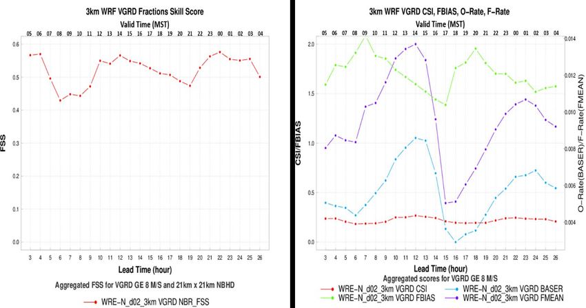
Contents

List of Figures                                                           v

List of Tables                                                           vi

Acknowledgments                                                         vii

Executive Summary                                                       viii

1.   Introduction                                                         1
     1.1 Army Numerical Weather Prediction (NWP) for Weather-Impacts
         Prediction                                                  1
     1.2 Evaluation of Army NWP Weather Forecasts                         1
     1.3 UnRestricted Mesoscale Analysis (URMA) Gridded Observational
         Ground Truth Data for NWP Evaluation                             2

2.   Design of the Assessment                                             5
     2.1 Verification Approach                                            5
     2.2 Verification Domains                                             6

3.   Generation of Assessment Data                                        7
     3.1 Model Evaluation Tools                                           7
     3.2 Assessment Data                                                  8
     3.3 Verification Data Preprocessing                                  9
     3.4 MET Grid-Stat Processing                                       10

4.   Analysis of Assessment Data                                        12
     4.1 1-km WRF Domain                                                12
     4.2 3-km WRF Domain                                                20

5.   Summary and Conclusion                                             28
     5.1 1-km WRF Domain                                                29
     5.2 3-km WRF Domain                                                29

                                     iii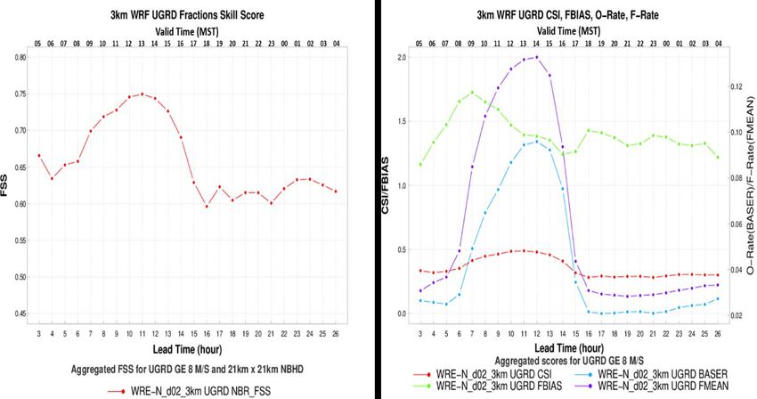
5.3 Both WRF Domains                                           30
     5.4 Future Work                                                31

6.   References                                                     33

Appendix. Fractions Skill Score (FSS), Critical Success Index (CSI),
    Frequency Bias (FBIAS), Observed Rate (O-Rate), and Forecast Rate
    (F-Rate) for U Wind Component (UGRD), V Wind Component
    (VGRD), and Specific Humidity (SPFH)                             37

List of Symbols, Abbreviations, and Acronyms                        44

Distribution List                                                   47

                                  iv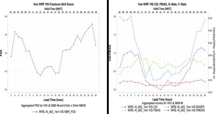
List of Figures
Fig. 1    Verification domains ............................................................................. 7
Fig. 2    Area covered by the 9-, 3-, and 1-km WRF domains ........................... 8
Fig. 3    Generation of verification-data flow diagram using the MET Grid-Stat
          tool ...................................................................................................... 10
Fig. 4    FSS, CSI, FBIAS, O-Rate, and F-Rate for 1-km WRF for freezing and
          above temperatures ............................................................................. 13
Fig. 5    FSS, CSI, FBIAS, O-Rate, and F-Rate for 1-km WRF for freezing and
          below temperatures ............................................................................. 13
Fig. 6    FSS, CSI, FBIAS, O-Rate, and F-Rate for 1-km WRF for DPT GE
          265 K................................................................................................... 14
Fig. 7    FSS, CSI, FBIAS, O-Rate, and F-Rate for 1-km WRF for DPT GE
          280 K................................................................................................... 15
Fig. 8    FSS, CSI, FBIAS, O-Rate, and F-Rate for 1-km WRF for WIND GE
          14 m/s .................................................................................................. 16
Fig. 9    FSS, CSI, FBIAS, O-Rate, and F-Rate for 1-km WRF for WIND GE
          18 m/s .................................................................................................. 16
Fig. 10   FSS, CSI, FBIAS, O-Rate, and F-Rate for 1-km WRF for TCDC GE
          25% ..................................................................................................... 17
Fig. 11   FSS, CSI, FBIAS, O-Rate, and F-Rate for 1-km WRF for TCDC GE
          50% ..................................................................................................... 18
Fig. 12   FSS, CSI, FBIAS, O-Rate, and F-Rate for 1-km WRF for VIS GE
          8000 m ................................................................................................ 19
Fig. 13   FSS, CSI, FBIAS, O-Rate, and F-Rate for 1-km WRF for VIS LE
          8000 m ................................................................................................ 19
Fig. 14   FSS, CSI, FBIAS, O-Rate, and F-Rate for 3-km WRF for TMP GE
          273 K................................................................................................... 21
Fig. 15   FSS, CSI, FBIAS, O-Rate, and F-Rate for 3-km WRF for TMP LE
          273 K................................................................................................... 21
Fig. 16   FSS, CSI, FBIAS, O-Rate, and F-Rate for 3-km WRF for DPT GE
          265 K................................................................................................... 22
Fig. 17   FSS, CSI, FBIAS, O-Rate, and F-Rate for 3-km WRF for DPT GE
          280 K................................................................................................... 23
Fig. 18   FSS, CSI, FBIAS, O-Rate, and F-Rate for 3-km WRF for WIND GE
          14 m/s .................................................................................................. 24
Fig. 19   FSS, CSI, FBIAS, O-Rate, and F-Rate for 3-km WRF for WIND GE
          18 m/s .................................................................................................. 24

                                                       v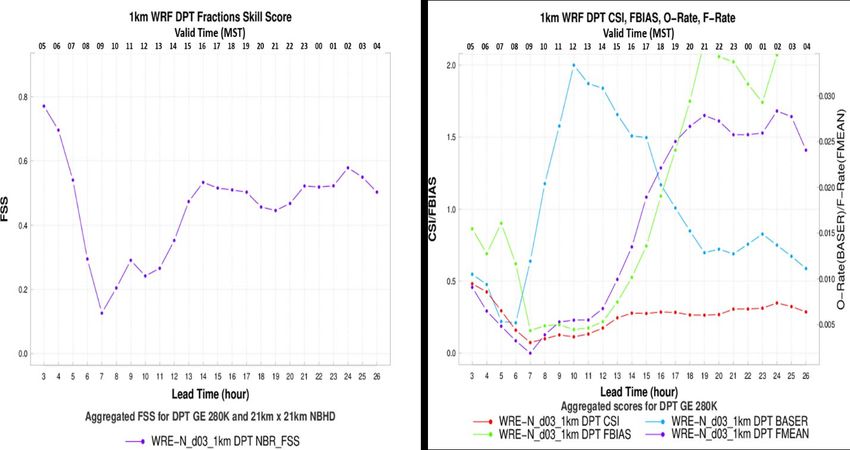
Fig. 20         FSS, CSI, FBIAS, O-Rate, and F-Rate for 3-km WRF for TCDC GE
                25% ..................................................................................................... 25
Fig. 21         FSS, CSI, FBIAS, O-Rate, and F-Rate for 3-km WRF for TCDC GE
                50% ..................................................................................................... 26
Fig. 22         FSS, CSI, FBIAS, O-Rate, and F-Rate for 3-km WRF for VIS GE
                8000 m ................................................................................................ 27
Fig. 23         FSS, CSI, FBIAS, O-Rate, and F-Rate for 3-km WRF for VIS LE
                8000 m ................................................................................................ 27
Fig. A-1        FSS, CSI, FBIAS, O-Rate, and F-Rate for 1-km WRF for UGRD GE
                0 m/s .................................................................................................... 38
Fig. A-2        FSS, CSI, FBIAS, O-Rate, and F-Rate for 1-km WRF for UGRD GE
                8 m/s .................................................................................................... 38
Fig. A-3        FSS, CSI, FBIAS, O-Rate, and F-Rate for 1-km WRF for VGRD GE
                0 m/s .................................................................................................... 39
Fig. A-4        FSS, CSI, FBIAS, O-Rate, and F-Rate for 1-km WRF for VGRD GE
                8 m/s .................................................................................................... 39
Fig. A-5        FSS, CSI, FBIAS, O-Rate, and F-Rate for 1-km WRF for SPFH GE
                0.002 Kg/Kg ........................................................................................ 40
Fig. A-6        FSS, CSI, FBIAS, O-Rate, and F-Rate for 1-km WRF for SPFH GE
                0.008 Kg/Kg ........................................................................................ 40
Fig. A-7        FSS, CSI, FBIAS, O-Rate, and F-Rate for 3-km WRF for UGRD GE
                0 m/s .................................................................................................... 41
Fig. A-8        FSS, CSI, FBIAS, O-Rate, and F-Rate for 3-km WRF for UGRD GE
                8 m/s .................................................................................................... 41
Fig. A-9        FSS, CSI, FBIAS, O-Rate, and F-Rate for 3km WRF for VGRD GE
                0 m/s .................................................................................................... 42
Fig. A-10 FSS, CSI, FBIAS, O-Rate, and F-Rate for 3-km WRF for VGRD GE
          8 m/s .................................................................................................... 42
Fig. A-11 FSS, CSI, FBIAS, O-Rate, and F-Rate for 3-km WRF for SPFH GE
          0.002 Kg/Kg ........................................................................................ 43
Fig. A-12 FSS, CSI, FBIAS, O-Rate, and F-Rate for 3-km WRF for SPFH GE
          0.008 Kg/Kg ........................................................................................ 43

List of Tables
Table 1         Near-surface meteorological and cloud-cover variables and threshold
                values used for the assessment ............................................................ 11

                                                            vi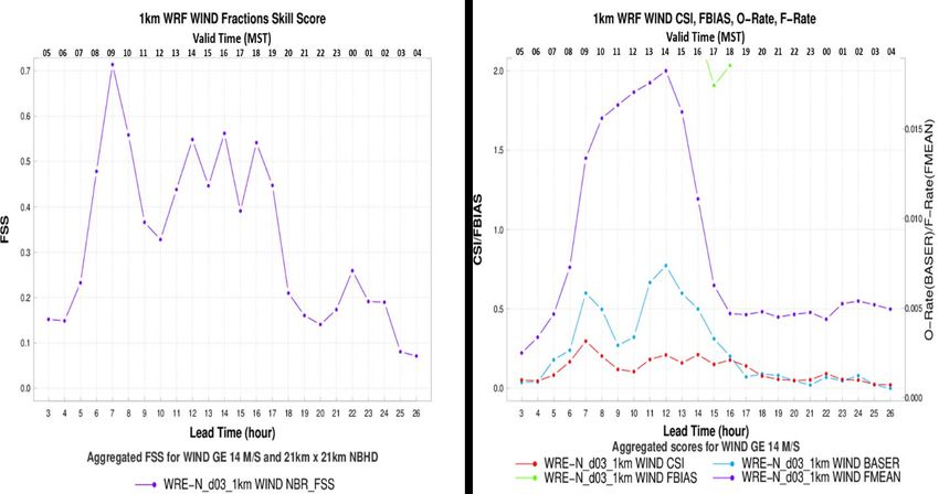
Acknowledgments

The authors would like to thank Dr Jeffrey A Smith for his review and suggestions
regarding the information presented on the Design of Experiments approach for
improving Numerical Weather Prediction (NWP) models. His contribution
enhanced the report by introducing a new and promising approach for model
improvement. The authors would also like to thank Mr Robert E Dumais Jr for his
thorough and thought-provoking review that resulted in numerous improvements
in the clarity and impact of this report. His comments suggested possibilities on
how this study could stimulate additional research into the use of verification of
high resolution NWP models for improving model forecasts. Many thanks to Ms
Sandra H Montoya of the US Army Combat Capabilities Development Command
Army Research Laboratory Technical Publishing for her attention to every detail in
the formatting and editing of this technical report.

                                       vii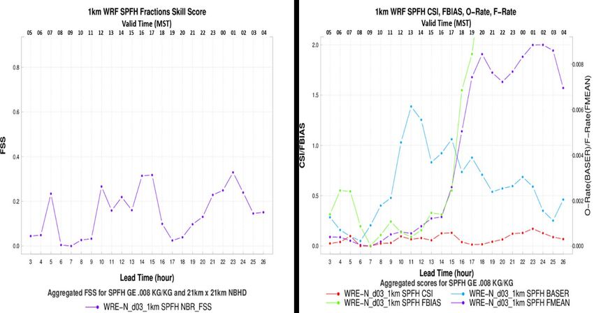
Executive Summary

An assessment of the Advanced Research version of the Weather Research and
Forecasting (WRF-ARW) model 1 was conducted over a winter-season 99-day
study period to quantify the accuracy of forecasts produced over the complex
terrain of the southwestern United States and northern Mexico. The study focused
on near-surface meteorological variables and cloud cover. Weather Research and
Forecasting–Chemistry (WRF-Chem) model 2 is a version of WRF-ARW that
contains a code module forecasting chemical constituents in addition to the standard
meteorological forecasts. This evaluation used outputs of WRF-Chem configured
to only include dust forecasts beyond the standard WRF-ARW fields (without
allowing dust to impact radiation); since dust is not evaluated in this study (and dust
does not affect other fields) the model used in the study will generally be referred
to as WRF-ARW, or more simply WRF. The model forecasts evaluated were
produced using the Weather Running Estimate–Nowcast Real-Time System
(WREN_RT), 3 which is a US Army Combat Capabilities Development Command
Army Research Laboratory-scripted system that performs data gathering, executes
WRF preprocessors, and runs WRF itself with the goal of supporting mission
planning and execution with high-resolution forecast information.
Weather-knowledge products for the Warfighters include forecasts of tactically
significant variables and decision-aid products that depict the 2-D distribution of
weather phenomena that can impact Army missions and systems. The WREN_RT
provides the forecasts that are ingested into the decision aids. The decision aids
apply weather thresholds to locate areas in time and space that exceed the thresholds
and indicate the possibility of significant impacts. To evaluate the accuracy of the
forecasts at the high resolutions of interest to the Army, high-quality gridded
observations are needed for ground truth to perform spatial verification. For this
assessment, the gridded observations used were the UnRestricted Mesoscale
Analysis (URMA) produced by the National Oceanic and Atmospheric
Administration for verification of Numerical Weather Prediction models. 4 The
assessment involved comparing forecasts produced by the WRF model with
1 Skamarock WC, Klemp JB, Dudhia J, Gill DO, Barker DM, Duda M, Huang XY, Wang W, Powers JG. A
description of the advanced research WRF version 3. University Corporation for Atmospheric Research; 2008.
Report No.: NCAR/TN-475+STR.
2 Grell GA, Peckham SE, Schmitz R, McKeen SA, Frost G, Skamarock WC, Eder B. Fully-coupled “online”

chemistry within the WRF model. Atmos Environ. 2005;39(37):6957–6975.
3 Reen BP, Dawson LP. The Weather Running Estimate–Nowcast Realtime (WREN_RT) system, version 1.03.

Army Research Laboratory (US); 2018 Sep. Report No.: ARL-TR-8533. https://apps.dtic.mil/sti/pdfs/
AD1060869.pdf.
4 De Pondeca Manuel SFV, Manikin G, DiMego G, Benjamin S, Parrish D, Purser RJ, Wu WS, Horel J, Myrick

D, Lin Y, et al. The real-time mesoscale analysis at NOAA’s National Centers for Environmental Prediction:
current status and development. Weather Forecast. 2011;26(5):593–612.

                                                  viii
URMA gridded observations over two domains located over the southwestern
United States and northern Mexico. This assessment has the benefit of a
significantly larger data set of input data compared with previous assessments that
were limited to periods of less than 30 days. This longer study period results in this
study having statistically stronger skill scores and statistics. The results of the study
show the accuracy of forecasts produced by the WRF for ingesting into decision
aids, and that the accuracy varies depending on the threshold used for determining
weather impacts.
ii1. Introduction
The Army requires weather-knowledge products to support the Intelligence
Preparation of the Battlefield process (ATP 2021) that is used to develop situational
understanding and identify those aspects of the operational environment that can
impact mission accomplishment. Weather systems can traverse multiple domains
interacting with the varied terrain and topography features to produce unique
conditions depending on location. Because multidomain operations rely on the
continuous integration of all domains of warfare, the commander must be aware of
the full spectrum of weather impacts across all domains produced by weather
phenomena from a wide range of spatial and temporal scales (TRADOC 2018).
These phenomena can range from large-scale areas of precipitation or dust storms
extending across hundreds of kilometers occurring over a period of 24 h or less to
erratic wind-flow patterns associated with dense urban environments that occur on
spatial scales of less than 1 km and time scales of a few minutes to 1 h.
1.1 Army Numerical Weather Prediction (NWP) for Weather-Impacts
Prediction
To address the need for the prediction of atmospheric conditions over multiple
domains, the Army has developed new NWP models and modified existing NWP
models that employ a range of grid sizes, initialization techniques, and
parameterizations to simulate weather phenomena across multiple spatial and
temporal scales. The Army Weather Running Estimate–Nowcast Real-Time
System (WREN_RT; Reen and Dawson 2018) executes the Advanced Research
version of the Weather Research and Forecasting (WRF-ARW; Skamarock et al.
2008) NWP model to provide the forecast grids that are ingested into the decision
aids. The decision aids apply thresholds to these forecasts to determine the spatial
and temporal distribution of weather conditions that can impact the effectiveness
of multidomain formations.
1.2 Evaluation of Army NWP Weather Forecasts
To evaluate the accuracy of the forecasts at the high resolutions of interest to the
Army, advanced methods of model verification are needed to verify high-resolution
output spatially as opposed to the more traditional methods that perform point-by-
point comparisons with observational ground-truth data coming from weather
observations. This grid-to-point approach to verification cannot adequately assess
the true skill of high-resolution forecasts.
1Traditional grid-to-point methods use point observations to verify the skill of NWP
models in predicting continuous meteorological variables by computing such
statistics as mean error and root-mean-square error, which characterize model
accuracy over the entire domain. When these techniques are applied to high-
resolution models such as the Weather Running Estimate–Nowcast (WRE–N), the
results can give misleading error estimates when compared with lower-resolution
models, which often score better when using these techniques. The issue is the
inability of the verification technique to evaluate the true skill of higher-resolution
forecasts, which replicate mesoscale atmospheric features in a way that is more
representative of the actual phenomenon owing to their use of a finer grid over
smaller domains, higher-resolution land-surface input data and models, and better
parameterization of subgrid physical processes (Jolliffe and Stephenson 2012).
In recent years, various nontraditional verification techniques were developed that
apply different approaches to show the value of higher-resolution forecasts. In
particular, spatial verification techniques have been developed that overcome the
limitations of grid-to-point techniques, which score on the basis of the exact
matching between point observations and the forecasts at those points. Fuzzy
verification, also known as neighborhood verification, is a spatial technique using
an approach that does not require exact matching and instead focuses on how well
the atmospheric feature or object is replicated by the model—even if there is a
spatial displacement of the feature. Ebert (2008) reviews a number of such methods.
The goal is to determine the amount of displacement by using a range of sizes of
neighborhoods of surrounding forecasts and observed grid points in the verification
process. In this way, model performance as a function of spatial scale can be
determined to allow selection of the scale required to have the desired accuracy.
These spatial verification methods require gridded observations instead of point
observations for ground truth.
1.3 UnRestricted Mesoscale Analysis (URMA) Gridded
Observational Ground Truth Data for NWP Evaluation
Sources of gridded observations are few, particularly at the spatial scale needed for
Army weather-knowledge products tailored for multidomain formations operating
in regions with varied and complex terrain conditions. For this study, the gridded
observations used were the UnRestricted Mesoscale Analysis (URMA) (De
Pondeca et al. 2011). URMA is used by the National Oceanic and Atmospheric
Agency (NOAA) National Weather Service (NWS) for verification of NWP
models. The Real-Time Mesoscale Analysis (RTMA), in conjunction with URMA,
provides real-time, 2-D meteorological gridded analysis products produced from
NWP analyses and hourly point weather observations from the national networks
2of Météorologique Aviation Régulière (METAR) and mesonet sensors that are
distributed over the continental United States (CONUS). Two-dimensional
RTMA/URMA was developed by National Centers for Environmental Prediction
(NCEP) in collaboration with the Earth System Research Laboratory and the
National Environmental, Satellite, and Data Information Service (De Pondeca et al.
2011). RTMA/URMA is produced on an hourly basis using a mesoscale analysis
background field produced from the 3-km High-Resolution Rapid Refresh (HRRR)
model and the 3-km North American Mesoscale model downscaled to the 2.5-km
grid as a first-guess background field (Morris et al. 2020). For the URMA products
used for this study, HRRR v2 on a 3-km grid was used (Benjamin et al. 2016). To
fill in gaps at the edges of the domain, the most recent forecasts from the Rapid
Refresh (RAP) were used (Morris et al. 2020). The RAP (RAP v3 for this study)
provides an hourly forecast on a 13-km grid over North America (Benjamin et al.
2016). The first guess field is then adjusted through a
2-D variational data assimilation technique (2DVAR) to analyze point weather
observations from the national networks of METAR and mesonet sensors (De
Pondeca et al. 2011). The first cycle of the analysis is the RTMA on a 2.5-km
CONUS grid that is used for weather situational awareness, calibration, and
aviation safety. URMA is produced by rerunning the RTMA on the same grid 6 h
following the first cycle to enhance the number of point observations used for
analysis to make it a better product for model verification/validation (Pondeca et
al. 2015). For example, NOAA uses URMA gridded observations for verification
and bias correction of the National Blend of Models used by NWS forecasters (Ruth
et al. 2017). URMA also serves as the NWS Analysis of Record (UCAR 2015). A
future development anticipated for the RTMA/URMA analysis system is the 3-D
RTMA, which is planned to provide 3-D analysis fields with subhourly updates
(Weygandt et al. 2019).
A number of studies have been conducted to compare the RTMA with observations.
Morris et al. (2020) reviews the results from a few such studies and presents the
results, which focused on performing an assessment of the RTMA to evaluate its
value as an alternative source of weather observations for use by airports for current
conditions affecting safety of flight. Their study consisted of running data-denial
experiments for retrospective periods of time that involved generating RTMA
output using specified ingest configurations. These configurations allowed the
assimilation phase to be controlled to restrict the available observational data to
create three distinct cases. The cases were 1) CONTROL case, which assimilated
all expected observations considered to be a more typical or normal scenario, 2)
EXP case, which denied access to observations coming from certain airports
considered to be a rare but not unprecedented scenario, and 3) NODA case that
denied access to all observations, which is considered to be the worst-case scenario.
3They determined the RTMA could be used as a substitute for airfield weather
observations under certain conditions, for only certain meteorological variables,
and only at certain locations. This is the most complete assessment compared to
any others investigated. The previous studies focused on evaluating the RTMA
using independent analyses products and controlled data-denial experiments and
not on providing a quantitative, grid-to-point verification over a longer, continuous
period of time.
To address the lack of a quantitative evaluation of URMA, Raby et al. (2020)
conducted an evaluation of the URMA during a continuous “winter” period from
11 Nov 2016 to 17 Feb 2017 over a large domain encompassing much of the
western United States, northern Mexico, portions of the Gulf of Mexico, Sea of
Cortez, and the eastern Pacific Ocean. This domain was also the outer nest region
(d01) for the WRF simulations produced during the same time period for included
subnests used in this study. The evaluation compared the URMA values for near-
surface meteorological variables to point observations of the same variables using
a traditional grid-to-point verification technique that generated continuous error
statistics over the 99-day time period. The results of the evaluation showed the
URMA provided a very-good analytical product for use as ground truth with certain
limitations. The limitations are attributable to 1) use of the grid-to-point verification
technique for high-resolution forecasts, and 2) use of point observations. This first
limitation refers to the requirement for exact matching between the forecast value
(in this case the URMA value) at the location of the point observation, which leads
to double-penalty errors for the forecast object being slightly displaced in space
from the observed object and gives no credit for a near-miss situation where the
forecast (URMA) object, despite replicating the observed object quite well
spatially, is displaced in location and/or time. The second limitation arises from two
sources. One source is that the URMA product is generated from the same point
observations that are being used for verification. The other source is the fact the
verification was conducted only at the locations in the URMA grid where there
were point observations and nowhere else, leaving areas where there is no
verification. The combined effect of these limitations on the accuracy of the URMA
error statistics generated from the evaluation is difficult to quantify, as well as their
impact on this assessment of WRF. That said, with no other source of better ground
truth and given the acceptance of URMA by NOAA as the analysis of record to be
used for verification, this study does provide reasonable evidence of the
performance of WRF based on a 99-day data set of simulation and URMA gridded
observational data.
42. Design of the Assessment
2.1 Verification Approach
The approach used for this objective assessment was spatial verification. The
specific techniques used were the neighborhood or “fuzzy” verification and
categorical verification. The neighborhood technique compared the model forecast
with the URMA gridded observations to determine the fraction of grid cells from
each exceeding a particular threshold within a given neighborhood size. The
resulting score is called the Fractions Skill Score (FSS; Roberts 2008; Roberts and
Lean 2008). For a given neighborhood size, each possible neighborhood of that size
within the evaluation domain is evaluated. By examining neighborhoods instead of
merely comparing grid points individually, the FSS is able to include the value of
near misses. A perfect forecast results in an FSS of 1.0. The FSS compares the
proportion of grid boxes within a forecast neighborhood that have events with the
proportion of grid boxes within the observed neighborhood that have events; this
results in a score that expresses the skill of the forecast by application of the
assumption that useful forecasts are those whose frequency of forecast events is
close to the frequency of observed events (Ebert 2008).
In this study we computed FSS for a range of neighborhood sizes and threshold
values to provide breadth in the FSS values to allow future analysis of the
dependency of FSS on those factors. For this report we selected one neighborhood
size with specific thresholds unique to each variable to provide some baseline
scores and statistics to characterize forecast accuracy of the WRF forecasts
produced over the middle (d02) and inner (d03) nests with grid spacing of 3 km and
1 km, respectively. The choice of neighborhood size was based on the “effective
resolution” considering the grid spacing of both nests and the lower bound for the
structure scale, which can be resolved by the nest with the largest grid spacing
(Skamarock et al. 2014).
We also computed related scores and statistics that are threshold dependent, based
on the categorical verification framework, but these are computed over the entire
domain and not computed using neighborhoods. These are the Critical Success
Index (CSI), frequency bias (FBIAS), observed rate (O-Rate), and forecast rate
(F-Rate). Traditional categorical verification scores and statistics are computed by
defining an event from both the forecast and the observation grids. The event is
defined by applying a threshold over the entire domain as the basis for determining
“hits” or “misses”, which follows the established theoretical framework for
evaluating deterministic binary forecasts. A CSI value of 1.0 indicates a perfect
forecast. O-Rate and F-Rate are fractional values of relative frequency of
5occurrence of the observed and forecast events ranging from 0 to 1 and FBIAS is
the ratio of the numbers of forecast events and the number of observed events. A
value of 1.0 for FBIAS is optimal, while less than 1.0 shows an underforecast
tendency and greater than 1.0 shows an overforecast tendency. This framework
evaluates the forecast skill by counting the numbers of times the event was
forecast—or not—and observed—or not—in a contingency table. Although
categorical scores and statistics have been widely used, they are not always reliable
for assessing the skill of high-resolution forecasts due to their sensitivity to
observed rate (Mittermaier et al. 2013). Raby (2016) determined that combining
categorical scores and statistics with those computed using a fuzzy verification
approach provides a more comprehensive assessment of model performance. To
overcome the limited applicability of scores and statistics generated from small data
sets for inferring information about the true accuracy of the model, Raby and Cai
(2016) suggested using a more rigorous approach that requires the generation of
larger data sets of forecast output and gridded observations so that more reliable
statistical results can be obtained. This approach is intended to improve the validity
of scores and statistics, particularly when observed event rates are low due to the
use of very-high or very-low threshold values of interest to the Army for predicting
impacts to systems and missions. For this reason, the decision was made to use
output from the WRF model, run on a daily basis producing 24 hourly forecasts
from 1200 to 1100 UTC, and the hourly URMA gridded observations for the same
hours over an extended time period. The period chosen was 11 Nov 2016 to 17 Feb
2017 because there were no significant changes made to the daily WREN_RT over
this time period and because of the availability of URMA gridded observations
produced using a single software version. This period contained 99 days that were
characterized as having typical “winter” conditions for the southwestern United
States and northern Mexico, and coincides with the period of the URMA evaluation
conducted by Raby et al. (2020).
2.2 Verification Domains
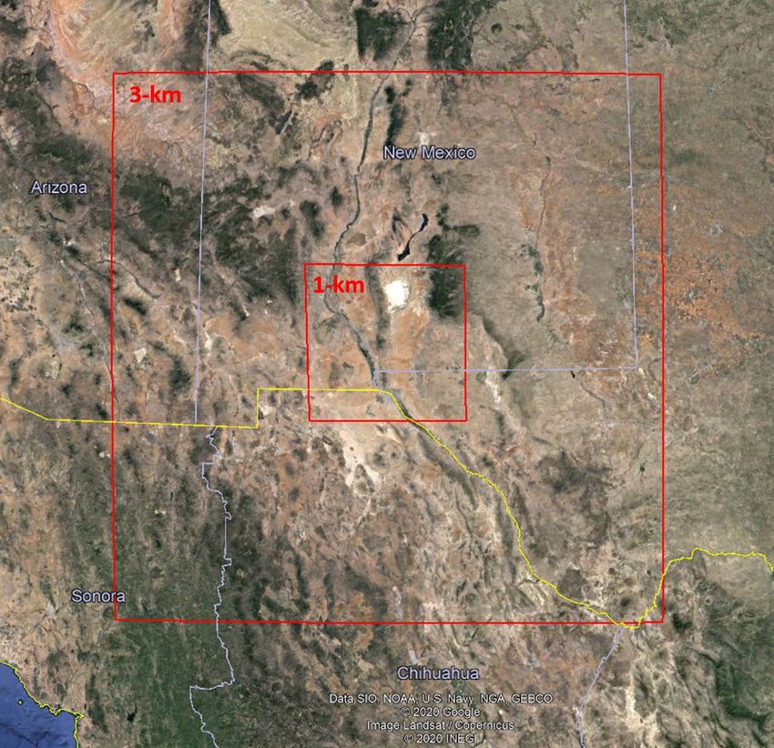
The two domains selected, shown in Fig. 1, were located over the southwestern
United States and northern Mexico. These domains were also the middle (3-km)
nest and the inner (1-km) nest for the WRF simulations produced during the 99-day
time period.
6Fig. 1 Verification domains
The verification was conducted over the two domains, both characterized by a
complex, mountain–desert–basin terrain landscape using hourly WRF forecasts and
URMA gridded observations collected for the 99-day “winter” period.
3. Generation of Assessment Data
3.1 Model Evaluation Tools
The software used to perform the scores and error statistic calculations was the
Model Evaluation Tools (MET) (Jensen et al. 2020). The MET was developed at
NCAR through grants from the United States National Science Foundation (NSF),
NOAA, the United States Air Force (USAF), and the United States Department of
Energy (DOE). NCAR is sponsored by the NSF. The output of MET was visualized
using the METviewer tool, also developed by NCAR. METViewer enabled the
aggregation of the error statistics over each lead time for all 99 days and then
produced plots of the statistics for each lead time.
73.2 Assessment Data
The URMA gridded observations used for this study were collected from the real-
time repository operated by the National Center for Environmental Prediction
(NCEP) (NOAA 2017).
The forecasts were created with WREN_RT using WRF-ARW V3.8 and the WRF
Pre-Processing System V3.8.1. Nested 9-, 3-, and 1-km horizontal grid spacing
domains centered just south of the White Sands Missile Range, New Mexico, were
executed for each day (Fig. 2) with 57 vertical full levels. The number of grid points
in the three domains are 9 km: 279 × 279, 3 km: 241 × 241, and 1 km: 205 × 205.
The 3-km domain covers about 12.4 times as much area as the 1-km domain, and
thus the 1- and 3-km domain overlap for only 8% of the area covered by the 3-km
domain. Each day a 3-h data-assimilation preforecast (0900–1200 UTC) preceded
a 24-h forecast from 1200–1200 UTC. (This study uses the 0–23 h forecast within
this period.)
Fig. 2 Area covered by the 9-, 3-, and 1-km WRF domains
Initial conditions were created by using Obsgrid (NCAR 2016) to perform
multiscan Cressman analyses with observations using 0.5-degree Global Forecast
8System model output as the first guess field. Observations were obtained from
NCEP’s Meteorological Assimilation Data Ingest System (MADIS;
madis.noaa.gov). Specifically, the MADIS surface, maritime, radiosonde, profiler,
and Aircraft Communications, Addressing, and Reporting System (ACARS) data
sets were used. In additional to being used in the analysis used in the initial
conditions, these observations were also applied in observation nudging data
assimilation (Reen 2016) during the preforecast from 0900 to 1200 UTC (the
nudging terms ramp down in the following hour after 1200 UTC, but no
observations valid after 1200 UTC are nudged towards). Observation nudging of
wind, potential temperature, and water vapor mixing ratio is applied with a
weighting of 6 × 10⁻⁴ s–1. The base horizontal radius of influence for the 9-, 3-, and
1-km domains are 120, 45, and 20 km, respectively, while the actual radius of
influence increases linearly with decreasing pressure to twice this value at 500 hPa
and is half this value at the surface. Observations are nudged in a 3-h time window
centered on the valid time of the observation with linearly decreasing temporal
weight in the outer half of the time window (for surface observations the time
window is two-thirds as large).
The planetary boundary layer scheme used was the Mellor-Yamada Nakanishi
Niino (MYNN) Level 2.5 scheme (with the MYNN surface-layer scheme).
Microphysics were parameterized using the Thompson aerosol-aware scheme. The
Grell–Freitas ensemble cumulus parameterization was used. For radiation, the
RRTMG (rapid radiative transfer model for general circulation models) shortwave
and longwave schemes were employed. The Noah land-surface model was used to
simulate the land surface. The simulations use WRF-Chem with dust-only enabled
using the Air Force Weather Agency’s dust scheme (WRF namelist settings
chem_opt = 401, dust_opt = 3); however, dust forecasts are not evaluated in this
report.
3.3 Verification Data Preprocessing
Some preprocessing tasks were completed before both the URMA gridded
observations and WRF forecasts for all 99 case-study days could be ingested into
the MET Grid-Stat tool to produce error statistics data, as shown in Fig. 3. The
scripts were developed and implemented in Python to make the preprocessing and
postprocessing tasks easier and more efficient resulting in the generation of
verification data that is better organized compared to running the tool on its own.
The 24 hourly URMA gridded observations in GRIB2 format from the evaluation
study described in Raby et al. (2020) were used as observation input into the MET
Grid-Stat tool. Next, the 24 hourly WRF forecasts were postprocessed using
Unified Post Processor (UPP) developed by NCEP (NCEP 2020) and a Python
9script, rename_upp.py, was used to rename each hourly, postprocessed WRF
forecast output file for all 99 case-study days to a standard filename convention.
Then, the renamed, postprocessed WRF forecasts were used as forecast input into
the MET Grid-Stat tool. Both the URMA gridded observation files and the
postprocessed WRF forecasts were ingested into the MET Grid-Stat tool using
another Python script, runGridStat.py, that performed the automation of the run and
data processes associated with the tool (Dawson et al. 2016).
Fig. 3 Generation of verification-data flow diagram using the MET Grid-Stat tool
3.4 MET Grid-Stat Processing
The MET Grid-Stat tool ingests the URMA gridded observations and the
postprocessed WRF forecasts so that matched pairs of forecast and observed values
for all the variables at each lead time can be processed over the 99-day period.
Because the URMA data is on a CONUS domain with 2.5-km grid spacing, Grid-
Stat regridded it to create domains with grids that matched the 1- and 3-km grids of
the WRF output to achieve the grid matching necessary for computing the forecast-
observation differences and error statistics. Grid-Stat applied the specified
neighborhood sizes (spatial scales) and thresholds and computed the neighborhood
10fractional coverage, contingency-table statistics, and skill scores for each spatial
scale.
The output of Grid-Stat consists of a tabular ASCII data formatted text file, called
STAT, which is used by other MET tools to access the fundamental data from
which the scores and error statistics are calculated. The STAT file contains 1) the
scalar partial sums generated during the calculation of the WRF–URMA
differences and 2) the contingency table counts and statistics for the entire domain
and for each neighborhood. For this study, the availability of the contingency table
counts in the hourly STAT files enabled their aggregation to produce the error
statistics and scores for each lead time over the entire 99-day period (Jensen et al.
2020). The METViewer software loads the STAT files, computes the FSS and other
error statistics according to user-specified settings by aggregating the data from all
the STAT files, and then generates plots of the statistics (NCAR 2018). Plots of the
statistics were generated for meteorological variables at the 2- and 10-m above
ground level (AGL) and cloud cover variables listed in Table 1.
Table 1 Near-surface meteorological and cloud-cover variables and threshold values used
for the assessment
Variable name/units Abbreviation Level (AGL) Threshold values
Temperature (degrees TMP 2m GE 273, LE 273
Kelvin [K])
Dew-point temperature DPT 2m GE 265, GE 280
(degrees K)
U wind component (m/s) UGRD 10 m GE 0, GE 8
V wind component (m/s) VGRD 10 m GE 0, GE 8
Wind speed (m/s) WIND 10 m GE 14, GE 18
Specific humidity SPFH 2m GE 0.002, GE
(kg/kg) 0.008
Total cloud cover (%) TCDC Entire GE 25, GE 50
atmosphere
Visibility (m) VIS Surface GE 8000, LE
8000
Threshold values used in this study are defined by the following acronyms:
“greater than or equal to” logical statement (GE)
“greater than” logical statement (GT)
“less than or equal to” logical statement (LE)
11“less than” logical statement (LT)
Some of the thresholds used in this study were values that have operational
significance due to their potential impact on aviation safety. For TMP, the
thresholds for approximately defining above- and below-freezing events were
selected. For WIND, the typical criteria for NWS issuance of wind advisories
(GE 14) and high-wind warnings (GE 18) were used. Note that criteria are subject
to variation by the local NWS office and are in mph (NOAA 2019).
For VIS, the thresholds used delineate the cutoff value separating the VIS criterion
for Visual Flight Rules (VFR) from the less favorable conditions of Marginal VFR
and potentially unfavorable conditions of Instrument Flight Rules (IFR). For cloud
cover, the thresholds used define the conditions of FEW (25%) or greater coverage
and SCT (50%) or greater coverage.
For the analysis of the output from MET Grid-Stat and METViewer, plots of the
FSS, CSI, O-Rate, and F-Rate for both WRF nested grids were generated to show
the trend as a function of lead time and Mountain Standard Time (MST). Note that
the middle WRF domain (d02) extends eastward into the Central Standard Time
zone. The readers are referred to the MET User’s Guide for the formulas used for
computing these statistics (Jensen et al. 2020).
4. Analysis of Assessment Data
4.1 1-km WRF Domain
The graphics showing the FSS, CSI, FBIAS, O-Rate, and F-Rate for all variables
for both thresholds and the analysis for the 1-km WRF domain are presented first
followed by those for the 3-km WRF domain. Figure 4 shows the 2-m-AGL TMP
scores for freezing and above temperatures and Fig. 5 shows the scores for freezing
and below temperatures for each model lead time for the 99-day period.
12Fig. 4 FSS, CSI, FBIAS, O-Rate, and F-Rate for 1-km WRF for freezing and above
temperatures
Fig. 5 FSS, CSI, FBIAS, O-Rate, and F-Rate for 1-km WRF for freezing and below
temperatures
The FSS scores in the left graphics (Figs. 4 and 5) are for a 21- × 21-km
neighborhood, which is somewhat larger than the “effective resolution” for a 1-km
grid spacing that is approximately 6–8 km. So the scores characterize the skill for
larger features that can be resolved relatively well by the WRF in this domain. For
above-freezing TMP, the FSS is perfect at all times. This is consistent with the CSI
and FBIAS values in the right graphics, which are very close to a perfect 1.0 value.
The O-Rate and F-Rate values show relative frequencies of occurrence of forecast
and observed events to be very high and nearly equal for the daytime period. At
13night, the frequencies differ with the F-Rate being slightly higher than the O-Rate,
which results in a slight over-forecast tendency. For below-freezing TMP, the FSS
is not as high, and varies widely over the diurnal period. The highest FSS scores
occur in the early morning, which is consistent with higher frequencies of
occurrence of O-Rate and is an indication that when below-freezing temperatures
are more likely to occur, the WRF in this domain shows good skill. This is also
reflected in the FBIAS values in the early morning, which are fairly close to 1.0.
From midmorning to midafternoon, the FSS is lowest with the FBIAS showing an
over-forecast tendency when the relative frequency of occurrence of observed
events is lowest. By early evening, the FSS has increased to show good skill as the
frequency of occurrence of observed events starts to rise and the over-forecast
tendency decreases to a value near 1.0. At night, there is a steady increase in the
frequency of occurrence of observed events into the early morning hours, but the
frequency of forecast events does not match this steady increase resulting in the
transition to an under-forecasting tendency and lower FSS values. The CSI for
below-freezing TMP is decidedly lower than for above-freezing TMP and remains
steady near a value of 0.5 over the 24-h period.
The graphics showing the FSS, CSI, FBIAS, O-Rate, and F-Rate for 2-m-AGL DPT
for the 1-km WRF for both thresholds are presented in Figs. 6 and 7, respectively.
Figure 6 shows the scores for DPT GE 265 K and Fig. 7 shows the scores for DPT
GE 280 K for each model lead time for the 99-day period.
Fig. 6 FSS, CSI, FBIAS, O-Rate, and F-Rate for 1-km WRF for DPT GE 265 K
14Fig. 7 FSS, CSI, FBIAS, O-Rate, and F-Rate for 1-km WRF for DPT GE 280 K
For DPT GE 265 K, the skill of the WRF is perfect, as indicated by the FSS being
1.0 and the CSI being very close to 1.0 over the 24-h period. The FBIAS values
show good agreement with the values being close to 1.0 over the diurnal period.
The overall tendency is for slight over-forecasting for most of the day except for
midmorning when the O-Rate and F-Rate are nearly equal, resulting in FBIAS
values being closest to 1.0. Despite FBIAS being close to 1.0 over the remaining
portions of the day, the O-Rate and F-Rate do not track each other very well, as was
the case for TMP, but the magnitude of their difference is not significant as
indicated by the FBIAS being close to 1.0. For DPT GE 280 K, the skill of the WRF
is not as good as that at the lower threshold as evidenced by the lower FSS and CSI
scores. The FBIAS values show an under-forecasting tendency in the early morning
to the late afternoon and then transitions to an over-forecasting tendency at night.
This transition is reflected in the behavior of the O-Rate and F-Rate with the former
increasing sharply during midmorning to a peak well above the latter by midday.
This is followed by a sharp decrease in O-Rate from the afternoon into nighttime
contrasted with a sharp increase in F-Rate during the same time period. Despite the
seemingly small differences in the values of O-Rate and F-Rate, the magnitude of
the FBIAS, before and after this transition, is relatively large.
The graphics showing the FSS, CSI, O-Rate, and F-Rate for 10-m-AGL WIND for
the 1-km WRF for both thresholds are presented in Figs. 8 and 9, respectively.
Figure 8 shows the scores for WIND GE 14 m/s and Fig. 9 shows the scores for
WIND GE 18 m/s for each model lead time for the 99-day period.
15Fig. 8 FSS, CSI, FBIAS, O-Rate, and F-Rate for 1-km WRF for WIND GE 14 m/s
Fig. 9 FSS, CSI, FBIAS, O-Rate, and F-Rate for 1-km WRF for WIND GE 18 m/s
For WIND GE 14 m/s, the FSS and CSI scores are fairly low, which is a reflection
of the impact of the threshold value that is sufficiently high to reduce the O-Rate to
very-low values over the 24-h period. This is consistent with the reduced incidence
of stronger winds over the 1-km domain in winter compared to other times of the
year. However, the WRF tended to over-forecast WIND over the entire period with
the FBIAS exceeding a value of 2.0 most of the time. This reduction in skill and
increase in over-forecast tendency is especially evident for WIND GE 18 m/s,
which shows extremely small values of O-Rate and F-Rate indicative of a situation
where there are only very limited areas when the threshold is exceeded and resulting
16in lower scores due to the difficulty imposed when scoring over limited areas
(Jolliffe and Stephenson 2012). Raby and Cai (2016) and Raby (2016) apply an
object-based analysis of the underlying cause of the lower skill scores, which is due
to the difficulty of matching smaller objects compared to larger objects. For smaller
objects, a displacement error can result in a significant decrease in the number of
hits and increases in the number of misses, which serves to lower scores compared
to larger objects that have more hits and less misses from the same displacement
error. Thus, the lower scores may not be totally attributable to the reduced skill of
the WRF in forecasting higher wind speeds.
The graphics showing the FSS, CSI, O-Rate, and F-Rate for TCDC for the 1-km
WRF for both thresholds are presented in Figs. 10 and 11, respectively. Figure 10
shows the scores for TCDC GE 25% and Fig. 11 shows the scores for TCDC GE
50% for each model lead time for the 99-day period.
Fig. 10 FSS, CSI, FBIAS, O-Rate, and F-Rate for 1-km WRF for TCDC GE 25%
17Fig. 11 FSS, CSI, FBIAS, O-Rate, and F-Rate for 1-km WRF for TCDC GE 50%
For TCDC, the two threshold values chosen represent the NWS criteria for defining
cloud-cover conditions of FEW (25%) or greater coverage and SCT (50%) or
greater coverage. For cloud cover, the O-Rates for both thresholds do not indicate
significant reduction of event frequency associated with increased threshold
magnitude as was the case for WIND, but the O-Rate for the higher threshold value
is lower than that of the lower threshold indicating a modest reduction in event
frequency. Overall, the FBIAS for TCDC GE 50 is better than that for TCDC GE
25, which is atypical compared to the other variables. The FBIAS values for both
thresholds show the strongest under-forecast tendency in the early morning
between 0500 to 0800 MST, followed by some improvement for the remainder of
the day. The FSS and CSI for TCDC at the lower threshold are not high, but are
better than those at the higher threshold. It is interesting to note the FSS score of
1.0 at 0500 MST. The low value of the CSI at this time (0.4) does not seem
consistent with the high FSS value. More investigation is needed to explain this
occurrence. It should be noted that these scores were computed using postprocessed
WRF output and not raw, prognostic WRF output. The UPP postprocessing
software uses an algorithm that calculates cloud cover from WRF prognostic
parameters and variables.
The graphics showing the FSS, CSI, O-Rate, and F-Rate for VIS for the 1-km WRF
for both thresholds are presented in Figs. 12 and 13, respectively. Figure 12 shows
the scores for VIS GE 8000 m and Fig. 13 shows the scores for VIS LE 8000 m for
each model lead time for the 99-day period.
18Fig. 12 FSS, CSI, FBIAS, O-Rate, and F-Rate for 1-km WRF for VIS GE 8000 m
Fig. 13 FSS, CSI, FBIAS, O-Rate, and F-Rate for 1-km WRF for VIS LE 8000 m
For VIS, the two threshold values chosen define the cutoff value separating the VIS
criterion for VFR from the less favorable conditions of Marginal VFR and
potentially unfavorable conditions of IFR. The FSS and CSI scores for VIS GE
8000 m are near perfect, while those for LE 8000 m are not as good. The overall
reduction in the scores for LE 8000 m, as compared with GE 8000 m, appears to be
related to the drastic reduction in the event frequency as indicated by O-Rate with
attendant smaller object sizes. For GE 8000 m, the FBIAS is very good with values
close to 1.0, but at LE 8000 m the values range between 0.5 and 0.8 indicating an
under-forecast tendency for lower VIS events. For lower VIS events, it is
19noteworthy that the lowest skill occurs during the afternoon hours as opposed to
the early morning hours. Reduction in VIS during the afternoon hours may be
associated with the occurrence of some blowing-dust events, which are relatively
infrequent during the winter months. Another factor contributing to this apparent
lack of skill might be the code used by the UPP for postprocessing the WRF output.
The VIS algorithm does not account for dust in its calculations; thus, even though
WRF was predicting a dust field (and outputting a VIS field based solely on dust),
this was not accounted for in the forecast VIS used for this verification. This, in
combination with the fact that the METAR VIS observations used in the URMA
analysis will necessarily include the effects of dust, may have contributed to this
apparent lack of skill in the afternoon hours.
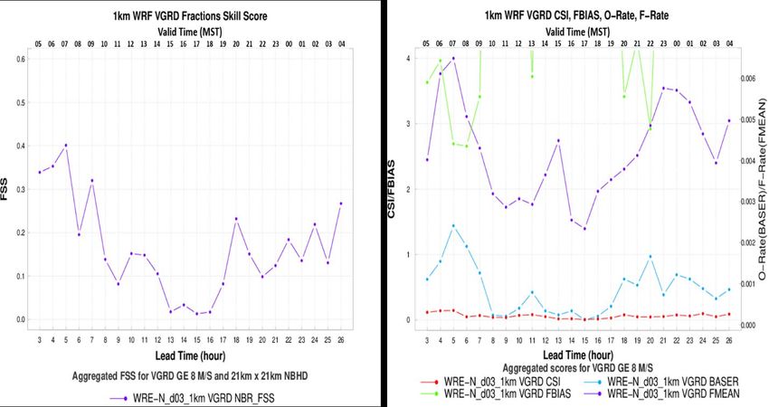
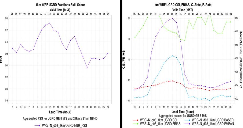
The scores and statistics for the remaining variables UGRD, VGRD, and SPFH all
present the same patterns in terms of high scores with lower thresholds and lower
scores with higher, event-limiting thresholds. Since there are no operational
thresholds for these variables, their scores will not be presented here, but are
presented in the Appendix.
4.2 3-km WRF Domain
The following graphics show the FSS, CSI, FBIAS, O-Rate, and F-Rate for all
variables for both thresholds and the analysis for the 3-km WRF domain. The
graphics showing the scores for TMP for both thresholds are presented in Figs. 14
and 15, respectively. Figure 14 shows the 2-m-AGL TMP scores for freezing and
above temperatures and Fig. 15 shows the scores for freezing and below
temperatures for each model lead time for the 99-day period.
20Fig. 14 FSS, CSI, FBIAS, O-Rate, and F-Rate for 3-km WRF for TMP GE 273 K
Fig. 15 FSS, CSI, FBIAS, O-Rate, and F-Rate for 3-km WRF for TMP LE 273 K
The FSS scores in the left graphics are for a 21- × 21-km neighborhood that is
within the “effective resolution” for a 3-km grid spacing, which is approximately
18–24 km, so the scores characterize the skill for smallest features that can be
resolved by the WRF in this domain. For above-freezing TMP, the FSS is near
perfect over the 24-h period. This is consistent with the CSI and FBIAS values in
the right graphics, which are very close to a perfect 1.0 value. The O-Rate and
F-Rate values show relative frequencies of occurrence of forecast and observed
events to be very high and nearly equal for the daytime period. At night, the
frequencies differ with the F-Rate being slightly higher than the O-Rate, which
results in a slight over-forecast tendency. For below-freezing TMP, the FSS is not
21as high and varies over the diurnal period. The highest FSS scores occur in the early
morning, which is consistent with higher frequencies of occurrence of O-Rate and
is an indication that when below-freezing temperatures are more likely to occur, the
WRF shows good skill. This is also reflected in the FBIAS values in the early
morning, which are fairly close to 1.0. From midmorning to late afternoon, for
below-freezing TMP, the FSS is lowest with the FBIAS showing an over-forecast
tendency when the relative frequency of occurrence of observed events is lowest.
By early evening, the FSS has increased to show good skill as the frequency of
occurrence of observed events starts to rise and the over-forecast tendency
decreases to a value near 1.0. At night, there is a steady increase in the frequency
of occurrence of observed events into the early morning hours, but the frequency
of forecast events does not match this steady increase resulting in the transition to
an under-forecasting tendency and slightly lower FSS values. The CSI for below-
freezing TMP is decidedly lower than for above-freezing TMP and remains steady
near a value of 0.6 over the 24-h period.
The graphics showing the FSS, CSI, FBIAS, O-Rate, and F-Rate for 2-m-AGL DPT
for the 3-km WRF for both thresholds are presented in Figs. 16 and 17, respectively.
Figure 16 shows the scores for DPT GE 265 K and Fig. 17 shows the scores for
DPT GE 280 K for each model lead time for the 99-day period.
Fig. 16 FSS, CSI, FBIAS, O-Rate, and F-Rate for 3-km WRF for DPT GE 265 K
22Fig. 17 FSS, CSI, FBIAS, O-Rate, and F-Rate for 3-km WRF for DPT GE 280 K
For DPT GE 265 K, the skill of the WRF is judged to be almost perfect as indicated
by the FSS being 1.0 and the CSI being very close to 1.0 over the 24-h period. The
FBIAS values show good agreement with the values being close to 1.0 over the
diurnal period. The overall tendency is for slight over-forecasting over most of the
day except for midmorning when the O-Rate and F-Rate are nearly equal resulting
in FBIAS values being closest to 1.0. Despite FBIAS being close to 1.0 over the
remaining portions of the day, the O-Rate and F-Rate do not track each other very
well as was the case for TMP, but the magnitude of their difference is not significant
as indicated by the FBIAS being close to 1.0. For DPT GE 280 K, the skill of the
WRF is not as good as that at the lower threshold as evidenced by the lower FSS
and CSI scores. The best skill is achieved in the early morning when the relative
frequency of these higher DPT values is at its lowest for the 24-h period. The
FBIAS values show an under-forecasting tendency in the early morning to the late
afternoon and then transitions to an over-forecasting tendency at night. This
transition is reflected in the behavior of the O-Rate and F-Rate with the former
increasing sharply during midmorning to a peak well above the latter by midday.
This is followed by a sharp decrease in O-Rate from the evening into early morning.
The F-Rate undergoes a similar pattern of an increase followed by a decrease, but
displaced later in time. Despite the seemingly small differences in the values of
O-Rate and F-Rate, the magnitude of the FBIAS before and after this transition is
relatively large.
The graphics showing the FSS, CSI, FBIAS, O-Rate, and F-Rate for 10-m-AGL
WIND for the 3-km WRF for both thresholds are presented in Figs. 18 and 19,
23You can also read