A comparison of apartment rent price prediction using a large dataset: Kriging versus DNN - arXiv
←
→
Page content transcription
If your browser does not render page correctly, please read the page content below

A comparison of apartment rent price prediction using
                 a large dataset: Kriging versus DNN

Hajime Seya
Departments of Civil Engineering, Graduate School of Engineering Faculty of Engineering, Kobe
University, 1-1, Rokkodai, Nada, Kobe, Hyogo, 657-8501, Japan,
E-mail: hseya@people.kobe-u.ac.jp; Tel.: +81-78-803-6278

Daiki Shiroi
Gunosy Inc., Roppongi Hills Mori Tower, 6-10-1, Roppongi, Minato, Tokyo, E-mail:
daikishiroi@gmail.com

Abstract
 The hedonic approach based on a regression model has been widely adopted for the prediction of real
 estate property price and rent. In particular, a spatial regression technique called Kriging, a method of
 interpolation that was advanced in the field of spatial statistics, are known to enable high accuracy
 prediction in light of the spatial dependence of real estate property data. Meanwhile, there has been a
 rapid increase in machine learning-based prediction using a large (big) dataset and its effectiveness
 has been demonstrated in previous studies. However, no studies have ever shown the extent to which
 predictive accuracy differs for Kriging and machine learning techniques using big data. Thus, this
 study compares the predictive accuracy of apartment rent price in Japan between the nearest neighbor
 Gaussian processes (NNGP) model, which enables application of Kriging to big data, and the deep
 neural network (DNN), a representative machine learning technique, with a particular focus on
 the data sample size (n = 104, 105, 106) and differences in predictive performance. Our analysis
 showed that, with an increase in sample size, the out-of-sample predictive accuracy of DNN
 approached that of NNGP and they were nearly equal on the order of n = 106. Furthermore, it is
 suggested that, for both higher and lower end properties whose rent price deviates from the
 median, DNN may have a higher predictive accuracy than that of NNGP.

Key Word: Apartment rent price prediction; Kriging; Nearest neighbor Gaussian processes
(NNGP); Deep neural network (DNN); Comparison

Acknowledgment
 This study was supported by the Grants-in-Aid for Scientific Research Grant No. 18H03628 and
 17K14738 from the Japan Society for the Promotion of Science. Furthermore, the “LIFULL
 HOME’S Data Set,” was provided for research purposes by LIFULL Co., Ltd. with the assistance of
 the National Institute of Informatics, Japan.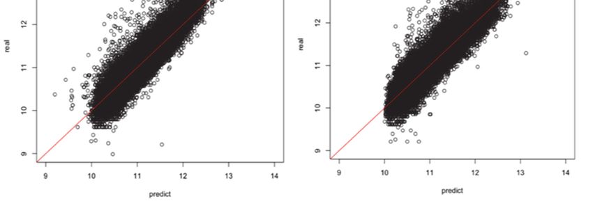
A comparison of apartment rent price prediction using

                           a large dataset: Kriging versus DNN

      1.    Introduction

           Real estate is an industry that has been said to relatively lag behind other businesses in

    terms of digitalization. During recent years, however, efforts to streamline operations using

    technologies have been gaining momentum. Online automated services for property price

    estimation is a recent technology and Zillow1, a service offered by Zillow Group in the US, is

    well known. Likewise, in Japan, there is a service termed Price Map2 from LIFULL. In Price Map,

    for example, properties are represented on a map with which one can review reference sale and

    rent prices by entering information such as room layout and lot size. Other similar services also

    exist and they are typically supported by huge property databases and statistics- or machine-learning-

    based sale and rent price prediction technologies. Against the backdrop of improved computer

    performance and expanded databases, these technologies have been termed as big data analysis or AI

    during recent years, and they are making rapid progress. As exemplified by the term ReTech, this has

    undoubtedly significantly impacted the real estate industry.

           Behind the increase in automated price assessment and prediction technologies using big

    data is the inefficiency of the current real estate industry. For example, in Japan, licensed real estate

    appraisers provide a property assessment based on an expected cash flows and comparison with

    similar properties. However, because all real estate properties have a uniqueness in the sense that

    there are no two identical properties and because an appraisal must be conducted considering the

    supply/demand balance, in addition to the property characteristics themselves, a tremendous effort

    must be made in explaining for the basis for the appraisal to consumers. Aside from appraisal costs,

    there is an issue of information asymmetry between real estate agencies and general consumers as

1   https://www.zillow.com/
2   https://www.homes.co.jp/price-map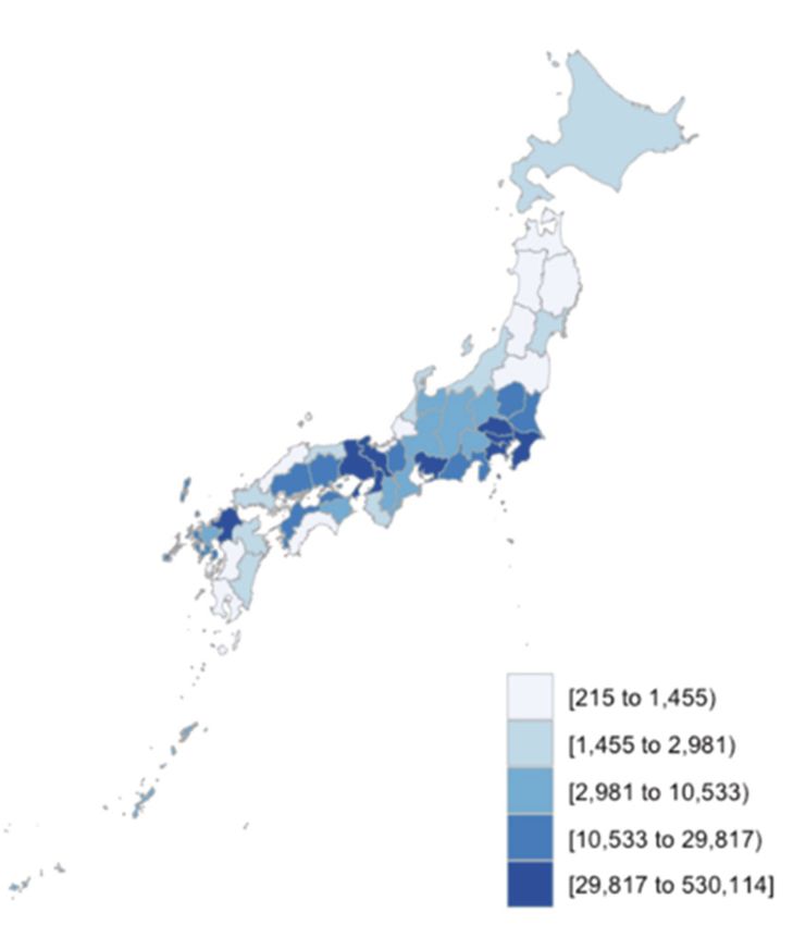
seen in the limited disclosure of purchase prices because of privacy policy3. This means that if real

 estate sale or rent prices can be reasonably and quickly predicted, then the information asymmetry

 between consumers and real estate agencies would disappear, leading to revitalization of the real-estate

 market. In other words, there is a need for an accurate prediction model of real estate sale and rent

 prices for businesses and consumers.

          While attention has been drawn to automated assessment of real-estate sale and rent prices

 using big data and machine learning techniques (Abidoye and Chan, 2017), conventionally, the

 hedonic approach has been widely used for predicting real estate sale and rent prices (Rosen, 1974).

 The hedonic approach takes the real estate sale or rent price to be a sum total of the values of

 attributes that comprise a property and typically estimates its price through regression analysis.

 Because it is an approach based on regression analysis, it can be implemented with relative ease and

 more importantly, marginal benefits of attributes can be evaluated using a calculated regression

 coefficient as a by-product. Meanwhile, from the perspective of prediction, simple functional forms such as

 logarithmic form or Box-Cox form are typically used4 . Thus, in a context where the sample size is

 sufficiently large, the big data plus machine learning approach, which can construct complex non-

 linear functions, is expected to outperform its alternatives. Indeed, as mentioned in the next section,

 several studies show this trend.

          For real estate appraisal, there are factors that are difficult to accommodate as explanatory variables

 such as local brand and historical context. It is therefore important to consider how these unobserved factors

 can be incorporated into the model. In spatial statistics, a method of handling these variables as the spatial

 dependence of error terms (neighboring properties are prone to a similar error), more strictly, a method of

 capturing spatial dependence by assuming a Gaussian process (GP), was established as Kriging (Dubin,

 1988). To name only a few, James et al. (2005), Bourassa et al. (2010), and Seya et al. (2011) have

 reported that Kriging provides high predictive accuracy compared to simple multiple regression

 models (hereinafter referred to as ordinary least squares (OLS)). Because model structure of OLS is

 rather simple, parameters can be properly set even with a relatively small sample size and there are

 not many benefits in using big data. By contrast, with Kriging, because pricing information of

 neighboring properties is reflected in the predicted results through spatial dependence, the situation is

3For example, although information on individual transactions of real estate properties is officially available in the Land

General Information System (http://www.land.mlit.go.jp/webland/) from the Ministry of Land, Infrastructure, Transport
and Tourism in Japan, location and price details are not available, and only approximate locations and prices are
available.
4 Semiparametric functional forms such as penalized spline can also be used (Seya et al., 2011).
different from that of OLS.
As previously noted, because the regression-based model can be used for evaluation, it is of high
practical use particularly in the social sciences. It is therefore important to test the extent to which its
predictive accuracy differs from that of the machine learning approach and understand the order.5 Thus, the
aim of this study was to compare and discuss the results of rent price prediction using three different
approaches—the [1] OLS, [2] spatial statistical (Kriging), and [3] machine learning approaches—for
various sample sizes. As the sample size increases, it is increasingly more difficult to straightforwardly
apply Kriging which requires the cost of O(n3) for inverting a variance–covariance matrix (for example,
when n = 105). Hence as a spatial statistical approach, the nearest neighbor Gaussian processes (NNGP)
model was used, which allows application of Kriging to big data (Datta et al., 2016; Finley et al., 2017;
Zhang et al., 2019). While there are various approaches for spatial statistical modeling using big data,
NNGP has been demonstrated to have better predictive accuracy and practicality in a
comparative study (Heaton et al., 2018).
As a machine learning approach, the deep neural network (DNN) was used. Neural networks
including the DNN are mathematical models of the information processing mechanism in the brain
composed of billions of neurons; multi-layered neural networks are termed the DNN. The DNN can
construct highly complicated non-linear functions and can consider spatial dependence through a
non-linear function for position coordinates without explicitly modeling the spatial dependence as in
the spatial statistical approach (e.g., Cressie and Wikle, 2011).
For validation, “LIFULL HOME'S Data Set”6, a data set for apartment rent prices in Japan
provided by LIFULL Co., Ltd. free of cost through the National Institute of Informatics, to
researchers, was used. Because there is generally less research regarding rental price than that
regarding sales price, it may be a valuable data set. The data set consists of snapshots (cross-section
data) that are either rental property data or image data as of September 2015. The former shows rent,
lot size, location (municipality, zip code, nearest station, and walk time to nearest station), year built,
room layout, building structure, and equipment for 5.33 million properties throughout Japan whereas
the latter is comprised of 83 million pictures that show the floor plan and interior details for each
property. In this study, only the former was used. One of our future tasks is to perform an experiment
using the latter.
5
There are models such as regression trees that are based on machine learning that can nevertheless provide useful
interpretations.
6 https://www.nii.ac.jp/dsc/idr/lifull/homes.htmlOut of approximately 5.33 million properties, 4,588,632 properties were obtained after
excluding missing data, from which n = 104,105, and 106 properties were randomly sampled. While
focusing on the difference in sample size, the accuracies of out-of-sample prediction for property rent
price based on approaches [1], [2], and [3] were compared through validation. The number of
explanatory variables K was 43 including constant terms. Our analysis showed that with an increase in
sample size, the predictive accuracy of DNN was observed to approach that of NNGP and on the order of
n = 106 they were nearly equal. During this experiment, standard explanatory variables that had been
incorporated into the regression-based hedonic model were used. Our findings suggested that, using these
standard settings, even if the sample size is on the order of n = 106, the use of regression-based NNGP is
sufficient.
In Chapter 2, we briefly review previous studies regarding related issues. Chapter 3 briefly explains
models used in this comparison study. Chapter 4 shows the results of the comparative analysis using the
LIFULL HOME'S data set. Lastly, Chapter 5 presents conclusions and provides future challenges to
address.
2. Literature review
This chapter offers a review of previous studies that compared the regression-based approach
and the neural-network-based approach in terms of prediction of real estate sale and rent prices.
Against, perhaps, readers’ anticipation, relatively limited research is available on this topic.
Kontrimas and Verikas (2011) compared the predictive accuracy of the machine-learning
approach including multi-layer perceptron (MLP), a subset of DNN, and OLS using data on home
sale transactions. They found that the mean absolute percentage difference (MAPD) for MLP and
OLS was 23% and 15%, respectively, and MLP was outperformed by OLS. However, the sample size
of their study was no greater than 100. Similarly, Georgiadis (2018) compared the predictive
accuracies of regression-based models and Artificial Neural Networks (ANN) on sales prices of 752
apartments in Thessaloniki, Greece, using cross valuation and found that the geographically weighted
regression model (Fotheringham et al., 2002) outperformed ANN. While these two studies have
shown that the regression-based approach outperformed the neural-network-based approach in terms ofpredictive accuracy, the sample sizes used for these studies were merely on the order of n = 102.
Meanwhile, Abidoye and Chan (2018) compared ANN and OLS using sales transaction
data for 321 residential properties in Lagos, Nigeria, and concluded that ANN outperformed
OLS. Likewise, Yalpır (2018) and Selim (2009) compared ANN and OLS and suggested that the
former performed better. Yalpır (2018) used 98 study samples, whereas Selim (2009) used fairly
large—5741 samples. In Yalpır (2018), they used three activation functions (the sigmoid, tangent
hyperbolic, and adaptive activation functions) to build ANN. However, hyperparameters other than
activation functions were fixed in validation.
As previously discussed, although several attempts have been made to compare and examine
the predictive accuracy of real estate sale and rent prices between a regression-based approach and a
neural-network-based approach, the results obtained were largely mixed. Limitations of previous
studies include [1] a small sample size (except for Selim (2009)), [2] disregard of spatial dependence
which is an essential characteristic of real-estate properties (except for Georgiadis (2018)), and [3]
tailored and ad hoc settings of hyperparameters in DNN (or ANN). To address these challenges, the
present study attempted to [1] perform an experiment at different and relatively large-scale sample
sizes (n = 104, 105, 106), [2] consider the spatial dependence either the application of NNGP (Kriging)
or the function of latitude/longitude coordinates (in case of DNN), and [3] optimize hyperparameters
in DNN.
3. Model
3.1. Nearest Neighbor Gaussian Processes (NNGP)
Let D be the spatial domain under study and let be a coordinate position (x, y coordinates).
Then, the spatial regression model, often termed as the spatial process model, can be expressed as
follows:
, ~ 0, , (1)
where is a variance parameter termed a nugget that represents micro scale variation and/or
measurement error. Normally, we assume that , where x is an explanatoryparameter vector at the point s and is the corresponding regression coefficient vector. is
assumed to follow the Gaussian process (GP) w ~ 0, ∙,∙ | , where the mean is zero and
the covariance function is ∙,∙ | ( is a parameter vector that normally includes the parameter
[where 1/ is called the range], which controls the range of spatial dependence, and the variance
parameter , which represents the variance of spatial process and termed partial sill). If a sample is
obtained at point s1, …, sn, w , ,…, follows the multivariate Gaussian
distribution:w~N(0, ), where the mean is zero and the covariance function is C(si, sj| ). Then
the spatial regression model can be expressed as y~N(X , , ), where
with I is an n n identity matrix. If the following relationship holds for any movement ∈ , w(s)
is considered a second-order stationarity spatial process.
0; ∀ ∈ , (2)
, | ;∀ , ∈ , (3)
, | ;∀ , ∈ . (4)
The second-order stationarity assumes that the covariance does not depend on position s and only
on h. When h depends only on the distance || || and not the direction, the spatial process is
said to have isotropy (||・|| is the vector norm). Covariance functions C(si, sj| ) that meet second-
order stationarity can be spherical, Gaussian, exponential, Matérn, etc. (Cressie, 1993).
The prediction of at any given point is termed Kriging 7 . The Kriging predictor
includes the n n variance-covariance matrix C with elements represented by C(si, sj| ) and the
calculation requires the cost of O(n3). The calculation will be difficult when n takes the value
around n = 105. By contrast, various approaches have been proposed that approximate the spatial
process w(s) (Heaton et al., 2018). Among other alternatives, this study used the NNGP model.
NNGP is based on Vecchia (1988) and assumes the following approximation to the joint
likelihood ∏ | , …, .8
∏ | . (5)
7Or , see Cressie (1993).
8Although the results depend on the ordering of the samples, Datta et al. (2016) showed that NNGP is insensitive to
ordering. We performed ordering based on the x-coordinate locations.Here, is a neighbors set of , and it is given as the k-nearest neighbors of in NNGP. Thus,
NNGP approximates the full GP expressed as a joint distribution using the nearest neighbors. Datta
et al. (2016) demonstrated that the approximation of formula (5) leads to approximation of the
precision matrix to provided in the following formula:
′ (6)
where A is a sparse lower triangular matrix with at most k-entries in each row and D = diag(dii) is a
diagonal matrix. Here, because A and D can be provided as m m matrices, it can significantly reduce
the computational load. The spatial regression model provided through NNGP may be written as
follows:
y~N(X , , ) (7)
where , .
The NNGP model parameters can be estimated using (Bayesian) Markov Chain Monte Carlo
(MCMC) (Datta et al., 2016), Hamiltonian Monte Carlo (Wang et al., 2018), and maximum
likelihood methods (Saha and Datta, 2018). This study uses MCMC. Because the NNGP parameters
are and , , ′ , ′, when using MCMC, we need to set a prior distribution for
each parameter and multiply it by the likelihood function to obtain conditional posterior distributions
(full Bayesian NNGP). Because this study addresses massive data up to a maximum of n = 106, it is
difficult to implement the full Bayesian NNGP within a practical computational time. Accordingly,
conjugate NNGP as proposed by Finley et al. (2017) was used. Suppose is a nearest
neighbors approximation of a correlational matrix corresponding to a nearest neighbors
approximation of a variance-covariance matrix— . Then the conjugate NNGP can be provided
as follows:
y~N(X , ) (8)
where and / . The point of using the conjugate NNGP is that, when
assuming that and are known, the conjugate normal-inverse Gamma posterior distribution for
and can be used and the predictive distribution for y( ) can also be obtained as a t-distribution;
thus, it is extremely easy to perform sampling.3.2. Deep neural network (DNN)
DNN is inspired by organism’s neural networks. It is a mathematical model that has a
network structure in which layered units are connected with neighboring layers. DNN allows
construction of extremely complicated non-linear functions. What follows is a schematic diagram
of a standard three-layered DNN created in reference to Raju et al. (2011):
[Figure 1: Three-layered feedforward neural network
(Created by author in reference to Raju et al. (2011))], around here
Each element that comprises a network is termed a unit or node and is represented as O (circle) in
Figure 1. The first layer is termed the input layer and the last the output; all of the other layers are
referred to as hidden layers. In DNNs, results of non-linear transformations on inputs received from
the previous layer are transmitted to the next layer to ultimately derive a single output as an
estimation result. In doing so, linear transformations via a weighted matrix ( )
and non-linear transformations via an activation function f(.) occur in each layer. The
transformation from the lth layer output zl ( 1) to the l + 1th layer output zl+1 ( 1)
can be computed according to the following formulas:
, 9
. 10
where b is a bias term. Suppose the number of layers is expressed as l = 1, …, L, output in the Lth
layer is the final output ( ≡ . f(.) is a non-linear function termed an activation function. Typical
activation functions include the sigmoid and Rectified Linear Unit, Rectifier (ReLU) functions; the
latter was used in this study. Any differentiable function can be used for the loss function of a DNN.
If regression is used as in this study, the Mean Squared Error (MSE) of the actual value and thepredictive value is often used.
1
11
For the loss function h, searching W and b that minimize h is termed DNN learning. Learning is
performed by the gradient algorithm, while backpropagation is used to calculate the gradient. In
contrast to the case of estimation, partial derivatives are computed in order from the output layer
(LeCun et al., 2011).
4. Comparison experiments: Kriging versus DNN
4.1. Dataset
As previously mentioned in Chapter 1, the LIFULL HOME’S data set was used in this study
for rent price prediction. Out of approximately 5.33 million properties, 4,588,632 properties obtained
by excluding missing data were used as original data. Although the original data did not explicitly
contain property positional coordinates s, they did contain zip codes and barycentric coordinates for
zip codes (X,Y coordinates of a WGS84 UTM54N type) were used on their behalf. This led to
inclusion of some positional errors in the positional coordinates. However, given that our study was
nationwide in scope, these errors are ignorable. The dependent variable is the natural logarithm of the
rent price (yen, including maintenance fees)) the explanatory variables shown in Table 1 were used.
The number of explanatory variables (K) was 43. Table 1 also shows descriptive statistics. Although the
classification of room layout in Table 1 could be more fine-grained, we used a slightly coarse classification
because we were more interested in comparing models than building a perfect hedonic model. Of all the
explanatory variables, information regarding use district (zoning) and floor-area ratio was often lacking in
the original database. Therefore, these data were separately prepared from the National Land NumericalInformation9. Figure 2 shows the number of properties per 1000 km2 and Figure 3 shows the natural
logarithm of the rent price (yen) for each prefecture.
[Table 1-1: Descriptive statistics (Continuous variables)], around here
[Table 1-2: List of explanatory variables (Discrete variables)], around here
[Table 1-3: Descriptive statistics (Discrete variables)], around here
[Figure 2: Number of properties per 1000 km2 for each prefecture], around here
[Figure 3: log (rent price) for each prefecture], around here
4.2. Experimental design
We compared the rent prediction accuracy based on three models: OLS, NNGP, and DNN.
For prediction, of 4,588,632 properties, properties were randomly selected at various sizes (n =104, 105,
106) and 80% of these data were used as training data for models for learning and the remaining 20%
were used as testing data (validation data) to test the prediction accuracy. The sample size for training and
testing data had three patterns: (8000 vs. 2000), (80,000 vs. 20,000), and (800,000 vs. 200,000). Because
sampling was completely randomly conducted, there were no containment relations such that, for
example, 104 samples are contained in 105 samples. However, because the data size was sufficiently big,
it would be highly unlikely that the sample bias would conceal trends, and thus this study design (based
not on conditionalization but on complete random sampling) would not greatly affect results.
For predictive accuracy assessment, the following error measures were used. Here, i, yi are
the out-of-sample predictive and observed values, respectively, for the ith data.
1
| | 12
1
13
1
14
9 http://nlftp.mlit.go.jp/ksj-e/index.html100
15
4.3. Model settings
4.3.1. OLS
OLS was added for comparison as a usual hedonic regression model that does not consider
spatial dependence. The explanatory variables are shown in Table 1 save the X and Y coordinates.
As a reference, Table 2 shows regression analysis results based on the OLS estimation when n = 106.
The adjusted R2 value was 0.5178 and fairly good given the sample size.
[Table 2: Regression analysis results using OLS (example of n = 106)], around here
4.3.2. NNGP
We used the conjugate NNGP proposed by Finley et al. (2017) as explained in Section
3.1. The conjugate NNGP is a pragmatic approach that accelerates sampling by assuming and
to be “known.” Needless to say, the full Bayesian NNGP is theoretically sound. In this study,
however, we addressed massive data with up to n = 106 of data; hence, it is practically difficult to
implement full Bayesian NNGP. In cases such as this, the conjugate NNGP offers a very useful
alternative. Finley et al. (2017) proposed to assign values to and via the grid point search
algorithm based on the cross-validation (CV) score. However, the computational load is high for
performing a grid point search for n = 106 of data. Therefore, in this study, the following simplified
10
procedure was undertaken in assigning values to and . From the remaining data that were not
used for comparison in this study, 10,000 properties were randomly sampled and parameters were
defined by iteratively re-weighted generalized least squares (Schabenberger and Gotway, 2005, pp.
256–259) in the semivariogram , which is in converse relation to the
covariance function. Figure 4 shows the fitting results. Starting from the left, the Gaussian,
spherical, and exponential models are shown. Of these, the Gaussian model had the best CV score,
and hence, was used. We can see that the Gaussian model is a particularly good fit to near-distance
10
One possible means to improve this is to apply the methods of hyper parameters value setting for the DNN as
mentioned in the next section. For the development of a concrete algorithm, we are leaving it for future study.that is subject to prediction results. Given these observations, the value for each parameter was as
follows: ϕ=1/25.8, τ 2 = 0.04, and σ2 = 0.03.
[Figure 4: Fitting of variogram functions
(Gaussian model; Spherical model; Exponential model)], around here
As a next step, the model parameters thus created were used to develop an NNGP
model. For implementation, the spConjNNGP function in the spNNGP package of R was used.
An NNGP model requires determining the number of nearest neighbors to consider. In the
default setting of the spConjNNGP function, it is 1511. When the relation between the number of
nearest neighbors k and CV score (MSE) was plotted12, there was a tendency for the MSE to
decrease to approximately k = 30 and then increase (Figure 5). Thus, the number of nearest neighbors
was set as k = 30 in performing the validation.
[Figure 5: Change in the MSE according to the number of nearest neighbors (in the case of n=105)]
4.3.3. DNN
This subsection explains the DNN settings. DNN has a number of parameters to be
determined, including the number of layers, the number of units in the hidden layers, learning rate,
and batch size. In addition, the DNN parameter space has a tree structure, which means that we must
be aware of the presence of conditional parameters. For example, the number of units in each layer
cannot be determined until the determination of the number of layers. The presence of these hyper
parameters is undoubtedly a source of the plasticity and high predictive accuracy of a DNN.
Conversely, there is no denying that the difficulty in and personalization of settings are obstacles for
applied researchers and practitioners who are interested in the prediction of real estate sale and rent
prices.
Thus, in this study, optimization for hyperparameters setting were considered. The grid and
11 In the default setting of the spConjNNGP function, the value is 15.
12 Because n = 104 and n = 106 did not produce large differences, the results of n = 105 are shown here.random searches are widely known as typical methods for DNN parameter tuning (Bergstra and
Bengio, 2012). In this study, a more efficient optimization technique known as the tree-structured
Parzen estimator (TPE) was adopted (Bergstra et al., 2011). The reason for adoption is its ability
to well address the tree-structured parameter space of DNNs and its numerous records of adoption
with proven performance to some degree (Bergstra et al., 2011; Bergstra et al., 2013). Nevertheless,
the parameter space (range of search) must be given a priori, and after much trial and error, it was
set as shown in Table 3.
[Table 3: DNN hyper parameter and search range], around here
ReLU 13 and MSE (refer to §3.2) were used for the activation function and loss function,
respectively. Regarding the optimizer for the DNN, because relatively large differences were found in the
results according to the type of algorithm used, results using typical algorithms, RMSprop (Tieleman and
Hinton, 2012) and Adam (Adaptive moment estimation) (Kingma and Ba, 2014), are shown.
Techniques designed to prevent overtraining such as regularized terms and dropout were not used
in this study. Keras 14 was used for the development of a DNN, and Optuna 15 , a framework
developed via Preferred Networks, Inc., was used for TPE implementation.
The learning procedure for a concrete model was undertaken as follows. First, based on the t th
hyper-parameter candidate vectors and the results of applying a five-fold cross validation with training
data for each (MSE, eq. (11)), a 50-fold search was performed using TPE. Second, a model was
created once again using the optimal hyper-parameter vector thus obtained and all the training
data to assess the predictive accuracy of the testing data. The explanatory variables used were
standardized in advance. Table 4 shows the optimization results of the hyper parameters.
[Table 4: DNN hyper parameters after optimization], around here
13 Historically, Sigmoid and Tanh were primarily used. Currently, ReLU has been accepted as a standard activation
function (LeCun et al., 2011).
14 https://keras.io
15 https://optuna.org4.4. Results
The predictive accuracies by sample size for each model are shown in Table 5.
[Table 5: Prediction results by sample size for each model], around here
As shown in Table 5, as a DNN optimizer, Adam had considerably higher predictive accuracy
compared to that of RMSprop. Therefore, for comparison to other models, Adam was used as a
reference. The predictive accuracies of OLS did not display large differences even if the sample size
increased. This would be because OLS, which did not use local spatial information, has a simple
model structure such that n = 104 was sufficiently large for determining parameters. NNGP
demonstrated the best results of all three models, for any sample size and any error measures. Even
with a relatively smaller sample size (n = 104), it showed high accuracy (MAPE = 1.152). At n =104,
DNN had a larger error than that of OLS when considering the root mean square error (RMSE)
(OLS: RMSE = 0.273, DNN: RMSE = 0.289). However, it had a larger margin of improvement in
accuracy with an increase in sample size, and at n = 106, it reached the same level as that of NNGP.
These results implied that DNN could be useful particularly in a context in which the sample size is
large. In other words, in a context in which the sample size is small, its predictive accuracy does not
differ much from that of OLS and this is considered to have led to the mixed findings of previous
studies as discussed in Chapter 2. Figure 6 shows scatter plots depicting predicted and actual rent
prices at n = 106.
[Figure 6: Scatter plot of predicted (horizontal axis) and actual (vertical axis) rent prices for each
model (in a case of n = 106)], around here
From Figure 6, we can see that, across all models, the predictive accuracy is poor particularly inareas where the rent price is high. To more closely evaluate, the MAPE per logarithmic rent price
range for each model is shown in Table 6. The comparison between NNGP and DNN shows that
DNN was more accurate in the high-rent areas with a logarithmic rent price of 12 or greater and
low-rent areas with a logarithmic rent price of 10-11. By contrast, NNGP performed better in the
median-rent areas with a logarithmic rent price of 11-12.
Table 7 shows the relative frequency of the prediction error: 100 % for n = 106.
According to Table 7, DNN had a higher percentage of samples with an error rate of 3.5% or greater
than that of NNGP (DNN: 2.461, NNGP: 2.133). Regarding the entire mean prediction result, DNN
and NNGP showed similar levels of accuracy (MAPE). These results suggest that DNN shows
robustness for rent price outliers but relatively high prediction errors in the vicinity of the median
(rent) value. However, NNGP tends to have low predictive accuracy for samples that deviate from
the median value. This would probably be because DNN is a non-linear model while NNGP is a
semi-log-linear model.
These results suggest that, regarding rent price prediction models using standard
explanatory variables, if the sample size is moderate (n = 104, 105), Kriging (NNGP) is useful,
whereas if a sufficient sample size is secured (n = 106), DNN may be promising.
[Table 6: MAPE per log (rent) range], around here
[Table 7: Relative frequency (%) (n=106) of prediction error rate (%)], around here
5. Concluding remarks
As mentioned in Chapter 1, there is a need for an accurate prediction model of real-estate sale
and rent price prices for businesses and consumers. The aim of this study was to compare and discuss
rent price prediction results based on regression approaches ([1] OLS and [2] spatial statistical approach
(Kriging)) and [3] the machine learning approach (DNN) using various sample sizes. As the sample size
increases (for example, n = 105), it is increasingly more difficult to straightforwardly apply Kriging which
requires the cost of O(n3) for the inverse matrix calculation of a variance–covariance matrix. Hence as a
spatial statistical approach, NNGP was used which allows application of Kriging to big data. For the
machine learning approach, DNN, a representative technique, was used. DNN can consider spatialdependence through a non-linear function for position coordinates without explicitly modeling the
spatial dependence as in NNGP.
For validation, from the “LIFULL HOME'S Data Set”16, a data set for apartment rent prices
in Japan—rent, lot size, location (municipality, zip code, nearest station, and walk time to nearest
station), year built, room layout, building structure, and equipment for approximately 5.33 million
properties across Japan—was used. To assess the effect that the sample size has on the difference in
predictive accuracy, properties with missing data were eliminated and then, n = 104, 105, and 106
properties were completely randomly sampled to compare the rent price prediction accuracy based on
approaches [1], [2], and [3]. The number of explanatory variables, K, was 43 including constant terms.
Our analysis showed that, with an increase in sample size, the predictive accuracy of DNN
approached that of NNGP and they were nearly equal on the order of n = 106. During this experiment,
standard explanatory variables that typically had been incorporated into the regression-based hedonic
model were used. It is no exaggeration to say that, under these standard settings, the use of regression-
based NNGP is sufficient even if the sample size is on the order of n = 106. Note, however, that DNN is
expected to be useful in contexts where K is even larger, e.g., when image data is used for explanatory
variables. The possibility of DNN must await further investigation.
In addition, regarding both higher-end and lower-end properties whose rent prices deviate from the
median, our study suggested that DNN may have a higher predictive accuracy than that of NNGP. This
is because unlike NNGP, DNN can explicitly consider the non-linearity of the function form.
Regarding this, the usefulness of the regression approaches that consider the non-linearity of the
function form, as in the geoadditive model (Kammann and Wand, 2003), was demonstrated by the
experiment conducted by Seya et al. (2011) using small samples. It will be worthwhile to test this
using big data in the future.
In this study, many DNN hyper parameters were determined using optimization techniques to
eliminate tailored and ad hoc setting as much as possible. Nevertheless, a certain portion of this
procedure, including the setting of parameter search range, had to depend on trial and error.
Because the difficulty of setting hyper parameters in DNNs poses an obstacle to their actual
operation for applied researchers and practitioners who are involved in the prediction of real estate
sale and rent prices, there is an urgent need to accumulate study results to resolve this issue.
Additionally, it is also important to establish an effective means to set NNGP hyper parameters.
16 https://www.nii.ac.jp/dsc/idr/lifull/homes.htmlReferences
Abidoye, R.B. and Chan, A.P. (2017) Artificial neural network in property valuation:
application framework and research trend, Property Management, 35(5), 554–571.
Abidoye, R.B. and Chan, A.P. (2018) Improving property valuation accuracy: a comparison
of hedonic pricing model and artificial neural network, Pacific Rim Property Research
Journal, 24 (1), 71–83.
Banerjee, S., Carlin, B.P. and Gelfand, A.E. (2014) Hierarchical Modeling and
Analysis for Spatial Data, Second edition, Chapman & Hall/CRC, Boca Raton.
Bergstra, J.S. and Bengio, Y. (2012) Random search for hyper-parameter optimization,
Journal of Machine Learning Research, 13, 281–305.
Bergstra, J.S., Bardenet, R., Bengio, Y. and Kégl, B. (2011) Algorithms for hyper-parameter
optimization, In Proceedings for Advances in Neural Information Processing Systems,
2546–2554.
Bergstra, J.S., Yamins, D., and Cox, D. (2013) Hyperparameter optimization in hundreds of
dimensions for vision architectures, In Proceedings for International Conference on
Machine Learning, 115–123.
Bourassa, S., Cantoni, E. and Hoesli, M. (2010) Predicting house prices with spatial
dependence: A comparison of alternative methods, Journal of Real Estate Research, 32 (2),
139–159.
Cressie, N. (1993) Statistics for Spatial Data, Wiley, New York.
Cressie, N. and Wikle, C.K. (2011) Statistics for Spatio-Temporal Data, John Wiley
and Sons, Hoboken.
Datta, A., Banerjee, S., Finley, A.O. and Gelfand, A.E. (2016) Hierarchical nearest-
neighbor Gaussian process models for large geostatistical datasets, Journal of the
American Statistical Association, 111 (514), 800–812.
Dubin, R.A. (1988) Estimation of regression coefficient in the presence of spatially
autocorrelated error terms, The Review of Economics and Statistics, 70 (3), 466–474.
Finley, A.O., Datta, A., Cook, B.C., Morton, D.C., Andersen, H.E. and Banerjee, S.
(2017) Applying nearest neighbor Gaussian processes to massive spatial data sets:
Forest canopy height prediction across Tanana Valley Alaska’(https://arxiv.org/pdf/1702.00434.pdf)
Fotheringham, A.S., Brunsdon, C. and Charlton, M. (2002) Geographically Weighted
Regression, John Wiley and Sons, Chichester.
Georgiadis, A. (2018) Real estate valuation using regression models and artificial neural
networks: An applied study in Thessaloniki, RELAND: International Journal of Real Estate
& Land Planning, 1, online.
Heaton, M.J., Datta, A., Finley, A.O., Furrer, R., Guhaniyogi, R., Gerber, F., Gramacy,
R.B., Hammerling, D., Katzfuss, M., Lindgren F., Nychka, D.W., Sun, F. and Zammit-
Mangion, A. (2018) A case study competition among methods for analyzing large
spatial data, Journal of Agricultural, Biological and Environmental Statistics, in print.
James, V., Wu, S., Gelfand, A. and Sirmans, C. (2005) Apartment rent prediction using
spatial modeling, Journal of Real Estate Research, 27 (1), 105–136.
Kammann, E.E. and Wand, M. P. (2003) Geoadditive models, Journal of the Royal
Statistical Society: Series C (Applied Statistics), 52 (1), 1–18.
Kingma, D.P. and Ba, J. (2014) Adam: A method for stochastic optimization. arXiv preprint
arXiv:1412.6980.
Kontrimas, V. and Verikas, A. (2011) The mass appraisal of the real estate by
computational intelligence, Applied Soft Computing, 11 (1), 443–448.
LeCun, Y., Bengio, Y. and Hinton, G. (2015) Deep learning. Nature, 521 (7553), 436.
Raju, M.M., Srivastava, R.K., Bisht, D., Sharma, H.C. and Kumar, A. (2011) Development
of artificial neural-network-based models for the simulation of spring discharge, Advances
in Artificial Intelligence, 2011, Article ID 686258, online.
Rosen, S. (1974) Hedonic prices and implicit markets: Product differentiation in pure
competition, Journal of Political Economy, 82 (1), 34–55.
Saha, A. and Datta, A. (2018) BRISC: Bootstrap for rapid inference on spatial
covariances, Stat, 7 (1), e184.
Schabenberger, O. and Gotway, C.A. (2005) Statistical Methods for Spatial Data
Analysis, Chapman Hall/CRC, Boca Raton.
Selim, H. (2009) Determinants of house prices in Turkey: Hedonic regression versus
artificial neural network, Expert Systems with Applications, 36 (2), 2843–2852.
Seya, H., Tsutsumi, M., Yoshida, Y. and Kawaguchi, Y. (2011) Empirical comparisonof the various spatial prediction models: in spatial econometrics, spatial statistics, and
semiparametric statistics, Procedia-Social and Behavioral Sciences, 120–129.
Tieleman, T. and Hinton, G. (2012) Lecture 6.5-rmsprop: Divide the gradient by a
running average of its recent magnitude, COURSERA: Neural Networks for Machine
Learning, 4 (2), 26–31.
Vecchia, A.V. (1988) Estimation and model identification for continuous spatial
processes, Journal of the Royal Statistical Society: Series B (Methodological), 50 (2),
297–312.
Wang, C., Puhan, M.A., Furrer, R. and SNC Study Group. (2018) Generalized spatial
fusion model framework for joint analysis of point and areal data, Spatial Statistics, 23,
72–90.
Yalpır, Ş. (2018) Enhancement of parcel valuation with adaptive artificial neural network
modeling, Artificial Intelligence Review, 49 (3), 393–405.
Zhang, L., Datta, A. and Banerjee, S. (2019) Practical Bayesian modeling and inference
for massive spatial datasets on modest computing environments, Statistical Analysis
and Data Mining, in print1
Tables
Table 1-1: Descriptive statistics (Continuous variables)
Min Max Median Mean SD
log(rent price) (yen) 8.57 20.9 11.1 11.1 0.402
Years built (month) 5 1812 228 236 135.6
Walk time to nearest (train) station (m) 1 88000 640 781.5 661.3
Number of rooms (#) 1 50 1 1.48 0.71
Floor-area ratio (%) 50 1000 200 234.1 130.6
X (km) -841 783.1 352.2 181.5 273.3
Y (km) 2958 5029 3931 3942 195.3
The “rent price” includes maintenance fees2
Table 1-2: List of explanatory variables (Discrete variables)
Direction North, Northeast, East, Southeast, South, Southwest, West, Northwest,
Other
Building W,B,S,RC,SRC,PC,HPC,
structure LS,ALC,RCB,Others
Room layout R, K, SK, DK, SDK, LK, SLK, LDK, SLDK
Category exclusively low residential zone (1 Exc Low), Category II
exclusively low residential zone (2 Exc Low), Category exclusively
Use district
high-medium residential zone (1 Exc Med), Category II exclusively high-
medium residential zone (2 Exc Med), Category I residential zone (1 Res),
Category II residential zone (2 Res), Quasi-residential zone (Quasi-Res),
Neighborhood commercial zone (Neighborhood Comm), Commercial zone
(Commercial), Quasi-Industrial zone (Quasi-Ind), Industrial zone
(Industrial), Exclusive industrial zone (Exc Ind), Others (Others)
For building structure: W: Wooden; B: Concrete block; S: Steel frame; RC: Reinforced concrete; SRC:
Steel frame reinforced concrete; PC: precast concrete; HPC: Hard precast concrete; LS: Light steel, RCB:
Reinforced concrete block
For room layout: The R refers to a room where there is only one room and there is no wall to separate the
bedroom from the kitchen. For the others, K: includes a kitchen; D: includes a dining room: L: includes a
living room; S: additional storage room. For example, LDK is a Living, Dining, and Kitchen area.
For use district: Category I exclusively low residential zone, Category II exclusively low residential zone,
Category I exclusively medium-high residential zone, Category II exclusively medium-high residential zone,
Category I residential zone, Category II residential zone, Quasi-residential zone, Neighborhood commercial
zone, Commercial zone, Quasi-industrial zone, Industrial zone, Exclusively industrial zone3
Table 1-3: Descriptive statistics (Discrete variables)
# denotes the number of cases
Direction Structure Use district Room layout
North 156843 W 1024081 1 Exc Low 780638 R 423815
Northeast 81173 B 570 2 Exc Low 25793 K 1729903
East 595252 S 844184 1 Exc Med 689879 SK 6919
Southeast 473041 RC 1892428 2 Exc Med 321441 DK 890584
South 1749315 SRC 190048 1 Res 1030319 SDK 5123
Southwest 458125 PC 11924 2 Res 211076 LK 516
West 404994 HPS 802 Quasi-Res 59863 SLK 138
Northwest 78836 LS 559974 Neighborhood Comm 386531 LDK 1505821
Others 591053 ALC 58373 Commercial 615630 SLDK 25813
RCB 597 Quasi-Ind 371672
Others 5651 Industrial 83826
Exc Ind 11949
Others 154
Table 2: Regression analysis results using OLS (example of n = 106)
Variable name Coef. t value
Constant term 10.81 4505
Years built -0.001155 -444
Walk time to nearest station -0.00004840 -98.3
Floor-area ratio 0.001294 228
Number of rooms 0.1486 257
Direction_Northeast 0.08202 28.3
Direction_East -0.006518 -3.41
Direction_Southeast 0.0008989 0.454
Direction_South -0.02640 -14.7
Direction_Southwest 0.001473 0.740
Direction_West 0.01494 7.49
Direction_Northwest 0.07861 26.9
Direction_Others -0.07103 -36.7
Structure_B 0.2078 7.00
Structure_S 0.09511 94.9
Structure_RC 0.2418 274
Structure_SRC 0.3670 206
Structure_PC 0.2161 35.1
Structure_HPC 0.1186 5.27
Structure_LS 0.05787 51.5
Structure_ALC 0.09498 32.9
Structure_RCB 0.08847 3.31
Structure_Others 0.1716 18.9
Room layout_K 0.0414 35.4
Room layout_SK 0.1010 12.5
Room layout_DK 0.1370 100
Room layout_SDK 0.3696 39.6
Room layout_LK 0.3052 9.87
Room layout_SLK 0.3322 5.82
Room layout_LDK 0.2765 213
Room layout_SLDK 0.5988 138
Use district_2 Exc Low -0.1231 -29.0
Use district_1 Exc Med -0.1494 -120
Use district_2 Exc Med -0.2747 -180
Use district_1 Res -0.2341 -196
Use district_2 Res -0.2444 -137
Use district_ Quasi-Res -0.2884 -98.4
Use district_ Neighborhood Comm -0.2594 -153
Use district_ Commercial -0.4571 -180
Use district_ Quasi-Ind -0.1891 -125
Use district_ Industrial -0.2451 -97.2
Use district_ Exc Ind -0.3047 -49.2
Use district_Others -0.3482 -1.76
Adjusted R2 0.51785
Table 3: DNN hyper parameters and search range
Hyper parameters Search range Type
# of hidden layers [1, 5] Integer
# of unites [10, 50] Integer
Batch size [32, 128] Integer
# of epochs [10, 30] Integer
Learning rate [10 , 10−2] (log)
−5 Real6
Table 4: DNN hyper parameters after optimization
n = 104 n = 105 n = 106
# of hidden layers 5 3 5
# of unites [46,16,32,30,43] [26,15,27] [37,22,24,31,50]
Batch size 33 45 125
# of epochs 15 19 25
Learning rate 0.009616156 0.005601793 0.0008054167
Table 5: Prediction results by sample size for each model
OLS NNGP DNN(Adam) DNN(RMSprop)
4
n = 10 MAE 0.215 0.127 0.212 0.227
MSE 0.074 0.032 0.083 0.102
RMSE 0.273 0.178 0.289 0.319
MAPE 1.938 1.152 1.920 2.041
5
n = 10 MAE 0.216 0.118 0.155 0.165
MSE 0.077 0.025 0.043 0.048
RMSE 0.279 0.159 0.208 0.219
MAPE 1.948 1.062 1.394 1.483
6
n = 10 MAE 0.217 0.112 0.114 0.132
MSE 0.078 0.024 0.025 0.033
RMSE 0.280 0.155 0.159 0.182
MAPE 1.955 1.013 1.031 1.1958
Table 6: MAPE per log (rent) range
Log(rent) OLS NNGP DNN
∼10 6.787 3.936 3.940
10∼10.5 3.456 1.704 1.508
10.5∼11 1.657 0.959 0.931
11∼11.5 1.602 0.852 0.920
11.5∼12 2.712 1.113 1.328
12∼12.5 4.718 1.784 1.734
12.5∼13 7.549 3.810 3.265
13∼ 13.505 8.335 7.7929
Table 7: Relative frequency (%) (n=106) of prediction error rate (%)
Prediction
OLS NNGP DNN
error rate %
0 ∼0.5 16.65 34.33 33.16
0.5 ∼1.0 15.77 26.38 26.49
1.0∼ 1.5 14.41 17.08 17.53
1.5 ∼ 2.0 12.52 10.1 10.09
2.0 ∼ 2.5 10.56 5.485 5.605
2.5 ∼ 3.0 8.646 2.919 3.026
3.0 ∼3.5 6.47 1.567 1.634
3.5 ∼ 14.98 2.133 2.461
Total (%) 100 100 1001
Figures
Figure 1: Three-layered feedforward neural network
(Created by author in reference to Raju et al. (2011))2 Figure 2: Number of properties per 1000 km2 for each prefecture
3

Figure 3: log (rent prices) for each prefecture
4

       Figure 4: Fitting of variogram functions
(Gaussian model; Spherical model; Exponential model)
5
Figure 5: Change in the MSE according to the number of nearest neighbors
(in the case of n=105)6
Figure 6: Scatter plot of predicted (horizontal axis) and observed (vertical axis) rent prices
for each model (in a case of n = 106)You can also read