A comparison of predicted and observed ocean tidal loading in Alaska
←
→
Page content transcription
If your browser does not render page correctly, please read the page content below
Geophys. J. Int. (2020) 223, 454–470                                                                                              doi: 10.1093/gji/ggaa323
Advance Access publication 2020 June 27
GJI Gravity, Geodesy and Tides

A comparison of predicted and observed ocean tidal loading in
Alaska
                           1
H.R. Martens                   and M. Simons2
1 Department   of Geosciences, University of Montana, Missoula, MT 59812, USA. E-mail: hilary.martens@umontana.edu

                                                                                                                                                             Downloaded from https://academic.oup.com/gji/article-abstract/223/1/454/5863947 by California Institute of Technology user on 21 July 2020
2 Seismological  Laboratory, Division of Geological and Planetary Sciences, California Institute of Technology, Pasadena, CA 91125, USA

Accepted 2020 June 24. Received 2020 June 24; in original form 2019 September 20

                                         SUMMARY
                                         We investigate the elastic and anelastic response of the crust and upper mantle across Alaska
                                         to mass loading by ocean tides. GPS-inferred surface displacements recorded by the Plate
                                         Boundary Observatory network are compared with predictions of deformation associated with
                                         the redistribution of ocean water due to the tides. We process more than 5 yr of GPS data from
                                         131 stations using a kinematic precise point positioning algorithm and estimate tidal contri-
                                         butions using harmonic analysis. We also forward calculate load-induced surface displace-
                                         ments by convolving ocean-tide models with load Green’s functions derived from spherically
                                         symmetric Earth models. We make the comparisons for dominant tidal harmonics in three
                                         frequency bands: semidiurnal (M2 ), diurnal (O1 ) and fortnightly (Mf ). Vector differences be-
                                         tween predicted and observed ocean tidal loading (OTL) displacements are predominantly
                                         sub-mm in magnitude in all three frequency bands and spatial components across the network,
                                         with larger residuals of up to several mm in some coastal areas. Accounting for the effects
                                         of anelastic dispersion in the upper mantle using estimates of Q from standard Earth models
                                         reduces the residuals for the M2 harmonic by an average of 0.1–0.2 mm across the network
                                         and by more than 1 mm at some individual stations. For the relatively small Mf tide, the effects
                                         of anelastic dispersion (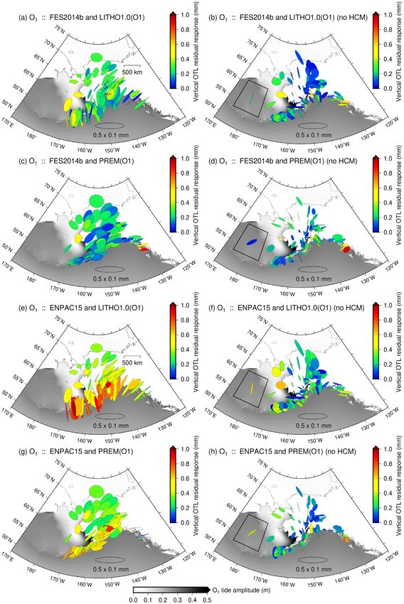
Ocean tidal loading in Alaska           455

                                                                        measure deformation with sufficient accuracy (e.g. Darwin 1898;
1 I N T RO D U C T I O N
                                                                        Farrell 1972b; Okubo & Saito 1983). Recent advances in satellite
Earth deforms in response to the redistribution of ocean water due      geodesy, however, including the proliferation of GNSS receivers
to tidal forcing in a process known as ocean tidal loading (OTL).       worldwide, have now made structural investigations tractable. Ito &
OTL-induced deformation can be measured using a variety of              Simons (2011) inverted residual OTL displacements in the western
geodetic techniques, including Global Navigation Satellite Systems      United States for refined elastic and density parameters through the
(GNSS), gravimeters, tiltmeters, strainmeters and very long base-       asthenosphere, albeit using a relatively short time span of data and
line interferometers (e.g. Baker 1984; Baker et al. 1996; Ito & Si-     without accounting for load-induced geocentre motions. Bos et al.
mons 2011; Yuan et al. 2013; Agnew 2015; Bos et al. 2015; Penna         (2015) used observations of OTL response in western Europe to

                                                                                                                                                 Downloaded from https://academic.oup.com/gji/article-abstract/223/1/454/5863947 by California Institute of Technology user on 21 July 2020
et al. 2015; Martens et al. 2016b). GNSS has emerged in recent years    probe upper mantle anelasticity at semidiurnal tidal periods. Yuan
as a preferred method for investigating tidally induced Earth defor-    et al. (2013) computed residuals between observed and predicted
mation (e.g. Agnew 2015). Advantages of GNSS include: receivers         OTL response for a global network of GNSS receivers and found
deployed around the world with a relatively high spatial density in     regional-scale spatial coherency, suggesting possible deficiencies
many regions; surface deformation monitored continuously at rel-        in the assumed spherically symmetric and elastic Earth model. An
atively high sampling rates (typically subsecond to 30-s intervals);    investigation into OTL response in South America also revealed
direct inference of surface displacements, rather than derivatives of   spatially coherent vector differences between OTL observations and
displacements (i.e. strain and tilt) that can be highly sensitive to    predictions, which were generally on the order of 0.3 mm or less
local structural variations; and processing methods capable of pro-     in all three spatial components of surface displacement (Martens
ducing precise estimates of surface displacement, typically on the      et al. 2016b). Moreover, Martens et al. (2016b) found similarities
order of 1 mm or better for each epoch (e.g. Agnew 2015; Herring        between predictions and observations even for the small-amplitude
et al. 2016).                                                           principal lunar fortnightly tide (Mf ), although measurement uncer-
   OTL-induced deformation is sensitive to both the distribution and    tainties were larger in this frequency band than for the semidiurnal
weight of the surface load as well as to the mechanical and density     and diurnal tides. Sensitivity analyses of Earth’s response to sur-
properties of Earth’s interior (e.g. Farrell 1972a; Agnew 2015). We     face loading indicate peak sensitivities to structure within the crust
can therefore use precise observations of OTL to constrain allow-       and upper mantle (Ito & Simons 2011; Martens et al. 2016a). As
able models for Earth structure as well as to refine models of the      such, OTL-induced deformation provides a valuable opportunity to
ocean tides. Ocean tides exhibit significantly greater spatial com-     perform inversions for structure using geodetic data sets that are
plexity than the solid-Earth body tides due to continental boundaries   complementary to traditional seismic methods.
and bathymetry, which interrupt the tidally driven flow of the wa-         Here, we perform a detailed case study of ocean tidal loading in
ter (e.g. Pugh & Woodworth 2014). The spatial complexity of the         Alaska using continuous GNSS data from the Global Positioning
ocean load allows the structure of the Earth to be sampled at a         System (GPS). We process the raw GPS data to derive time-series of
wide variety of spatial wavelengths, including at shallower depths      surface displacements with subdaily resolution in three dimensions
important to mantle convection and plate tectonics. Body tides are      (east, north and up). We then perform a tidal harmonic analysis to
long-wavelength features that sample larger scale averages of Earth     estimate the amplitudes and phases of individual tidal harmonics,
structure with sensitivity to deep-Earth properties (e.g. Latychev      taking care to correct for harmonic modulations and non-linear ef-
et al. 2009; Lau et al. 2017). Moreover, the broad temporal spec-       fects in shallow water. We then compare the observed OTL surface
trum of the total ocean tide allows the deformation response of the     displacements with forward calculations of deformation in three
Earth to be probed across a range of periods between characteristi-     tidal-frequency bands: semidiurnal, diurnal and fortnightly. Since
cally seismic (seconds to hours) and glacial (thousands of years).      tidal patterns are similar within each frequency band, we consider
   On average, tidal height variations in the ocean reach up to a few   only a dominant tidal harmonic from each band: the principal lunar
meters and amplitudes of surface displacements caused by OTL            semidiurnal harmonic, M2 , with a period of 12.42 hr; the principal
reach up to several centimeters in coastal areas (e.g. Lyard et al.     lunar diurnal harmonic, O1 , with a period of 25.82 hr; and the prin-
2006; Ito & Simons 2011; Yuan et al. 2013; Bos et al. 2015; Martens     cipal lunar fortnightly harmonic, Mf , with a period of 13.66 d. We
et al. 2016b). Ocean-tide models, constrained in part by satellite      then interpret the residual displacements in the context of GPS un-
measurements of sea-surface height, are now highly accurate in the      certainty estimates, modelling assumptions, ocean-tide distribution
deep ocean and no longer considered to be a dominant source of          and regional Earth structure.
error in OTL analyses in most regions (e.g. Stammer et al. 2014;           Ocean tidal loading has previously been explored in Alaska, al-
Bos et al. 2015; Martens et al. 2016b). The accuracy of ocean-          beit with a limited number of stations, short record lengths, outdated
tide models generally becomes degraded around complex coastlines        ocean-tide models, and a focus on only the semidiurnal tidal species.
and shallow seas, where satellite measurements are challenging and      Khan & Tscherning (2001) and Khan & Scherneck (2003) inves-
non-linear effects become important (e.g. Egbert et al. 2010; Pugh      tigated Earth’s displacement response to semidiurnal ocean tidal
& Woodworth 2014; Stammer et al. 2014). Furthermore, ocean-             loading at two GPS stations in Alaska over a period of 49 d, and
tide models are generally specified on regular, global grids with       found discrepancies between observations and predictions of about
resolutions that do not precisely match the geometries of intricate     2 mm in the up component and 1 mm in the north component for the
coastlines. Large vector differences between OTL observations and       M2 harmonic. Zürn et al. (1976) considered discrepancies between
predictions, particularly in coastal areas (e.g. Khan & Tscherning      the observed and modelled gravity response of the Earth to direct
2001; King et al. 2005; Martens et al. 2016b), present opportunities    tidal forcing at five gravimeter stations in southern Alaska, and
to use geodetic data to further refine the ocean-tide models.           found that much of the residual could be explained by the effects of
   Also of interest is using geodetic observations of OTL response      ocean tidal loading. We build upon and modernize the prior studies
to constrain allowable models for Earth structure (Ito & Simons         by processing data from 131 GPS receivers in the Plate Boundary
2011; Bos et al. 2015; Martens et al. 2016a, 2019). The theory          Observatory (PBO) network throughout Alaska for a period of over
behind load-induced Earth deformation long predates the ability to      5 yr: 1 January 2012 to 28 February 2017. Fig. 1(a) shows the
456       H.R. Martens and M. Simons

                                                                                                                                                                     Downloaded from https://academic.oup.com/gji/article-abstract/223/1/454/5863947 by California Institute of Technology user on 21 July 2020

Figure 1. (a) Map of Alaska showing GPS station locations and key geographic regions. GPS stations considered in our analysis are plotted as coloured
dots. The red dot denotes the station considered in panel (b). The yellow dots denote stations that are excluded from statistical and comparative analyses of
predictions and observations due to anomalous signals in the time-series; predictions and observations for all stations shown in the map are provided in the
Supporting Information. (b) GPS-inferred displacement time-series and tidal-harmonic model fit for PBO station AC79, which is located on Montague Island
in the Gulf of Alaska. The tidal-harmonic fit has been made to the full time-series of processed data (≈5 yr), but the figure shows an arbitrary snapshot of one
week from summer 2014. The panels on the left side depict the GPS time-series: the upper two panels show the east component of displacement; the centre
two panels show the north component of displacement; and the bottom two panels show the up component of displacement. For each pair, the top panel shows
the GPS time-series for the station (blue dots) at 5-min temporal resolution with the tidal-harmonic fit to the data overlaid (red line). The bottom panel in each
pair shows the residual time-series after the fitted tidal harmonics are removed (black dots). The panels on the right side depict residual displacements in the
east (top panel), north (middle panel) and up (bottom panel) components for the full time-series (≈5 yr). The residual value at one standard deviation from the
mean is annotated on each panel. Particularly for long data records, estimates of uncertainties for individual tidal harmonics (eqs 2 and 3) can be much less
than the standard deviation for all residuals due to the periodicity of the tides.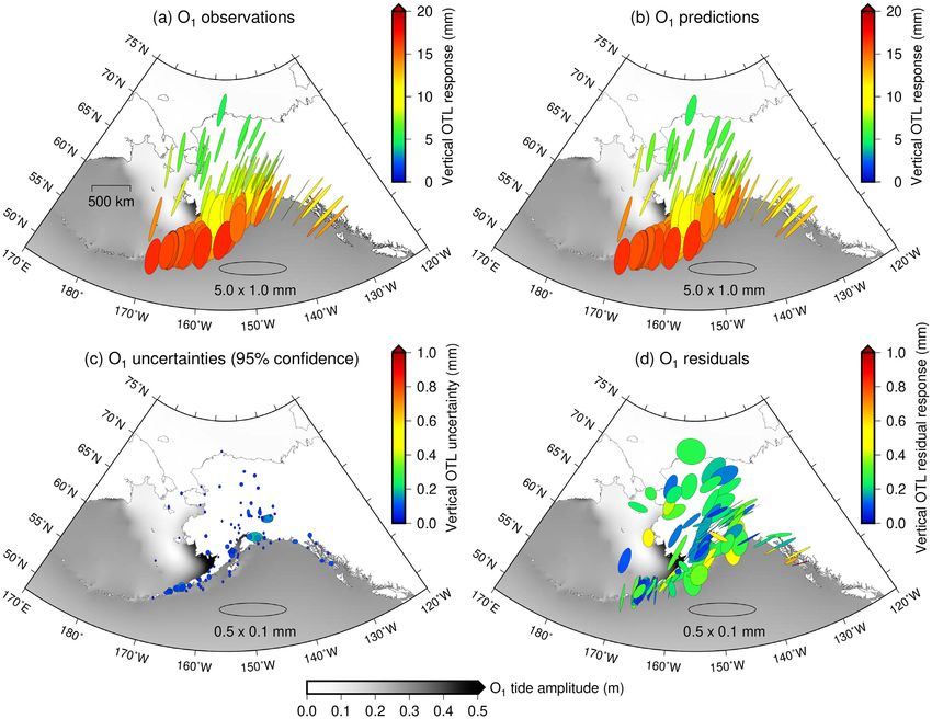
Ocean tidal loading in Alaska        457

Alaska network along with key geographic locations. We consider             lower elevations using the VMF1 mapping functions. We then es-
three distinct tidal species (semidiurnal, diurnal and fortnightly)         timate the tropospheric zenith delay stochastically, simultaneously
as well as all three displacement components (east, north and up).          with the coordinate positions, relative to the nominal delay values
                                                                                                                                  −1
Furthermore, we take advantage of contemporary, high-resolution             using a process noise setting of 5.0 × 10⁻⁸ km s 2 (cf. Martens
ocean-tide models to generate improved predictions of Earth’s re-           et al. 2016b). Horizontal gradients in the tropospheric wet delay
sponse to OTL. We also explore a range of different ocean-tide              are also estimated stochastically using a process noise setting of
and Earth-structure models, and evaluate the discrepancies between                              −1
predictions and observations for each model pair.                           5.0 × 10⁻⁹ km s 2 (Bar-Sever et al. 1998). Furthermore, we apply
                                                                            2nd-order corrections to the signal-propagation delay through the
                                                                            ionosphere with an effective shell height of 600 km.

                                                                                                                                                      Downloaded from https://academic.oup.com/gji/article-abstract/223/1/454/5863947 by California Institute of Technology user on 21 July 2020
2 K I N E M AT I C G P S P R O C E S S I N G
Standard GPS-processing methods involve modelling and removing              3 T I D A L H A R M O N I C A N A LY S I S
both the solid Earth tides and the ocean load tides prior to estimating
                                                                            We use the analysis methods described in Martens et al. (2016b)
receiver positions, most often using a static parameter-estimation
                                                                            to estimate the tidal harmonics in three dimensions (east, north
approach (e.g. Herring et al. 2016). Here, we seek to retain the ocean
                                                                            and up). We model the total tidal displacement for each spatial
load tides in the GPS time-series and estimate the load-tide har-
                                                                            component as a function of time, P(t), as a sum of sinusoids:
monics at the post-processing stage using harmonic-analysis tech-
niques. We therefore developed a custom GPS-processing strategy
                                                                                     N

for the specific purpose of analysing OTL-induced deformation,              P(t) =         cn f n (t) cos(Vn (t) + u n (t))
which closely follows the methods of Martens et al. (2016b). In                      n=1

particular, we process the raw RINEX-formatted GPS data using                        + sn f n (t) sin(Vn (t) + u n (t)),                       (1)
the GIPSY software (version 6.4), which uses a precise point posi-          where cn and sn are the in-phase and quadrature amplitudes of
tioning algorithm (Zumberge et al. 1997).                                   tidal harmonic n, Vn is the astronomical argument, N is the total
   The 15-s data are processed in kinematic mode to estimate re-            number of harmonics considered, t is time and fn and un are the
ceiver positions at 5-min intervals. Using GIPSY, we remove the             nodal factors needed to express modulation of the tidal harmonic
solid-Earth body and pole tides according to calculations provided          (Foreman et al. 2009; Martens et al. 2016b). We evaluate V, f and
by the International Earth Rotation Service (IERS, Petit & Luzum            u at each epochin the time-series. The amplitudes and phases are
2010). We do not model and remove the ocean load tides. Station             given by An = cn2 + sn2 and φ n = atan2(sn , cn ), respectively.
positions are estimated stochastically using a random-walk proce-              For the selection of primary harmonics to include in the inver-
                                                                     −1
dure with a coordinate process noise setting of 5.7 × 10⁻⁷ km s 2 ,         sion, we consider the Rayleigh frequency-resolution criterion with
which is a GIPSY-recommended value for slow-moving platforms                a cut-off value of 1.1 cycles for the Rayleigh parameter (e.g. Godin
(software documentation) and also consistent with the synthetic             1972; Foreman 1977). Harmonics with the largest equilibrium-
tests of Martens et al. (2016b).                                            tide amplitudes are prioritized over smaller-amplitude harmonics
   Nominal station positions are first obtained from the headers of         within the same frequency band. We base the amplitude rankings
RINEX files, and then updated after a preliminary run of GIPSY for          on the Cartwright–Taylor–Edden (CTE) equilibrium tide catalogue
each station. In order to mitigate potential inaccuracies in position       (Cartwright & Taylor 1971; Cartwright & Edden 1973).
estimation at the start and end of each day, we process data in 30 hr          In shallow seas and estuaries, non-linear effects can become im-
batches (i.e. a full day plus 3 hr on either side of the day) and extract   portant due to the increasing influence of friction between the water
only the central 24 hr of position estimates. We use precise satellite      and the sea floor (e.g. Pugh & Woodworth 2014). We account for
orbit and clock products from the Jet Propulsion Laboratory (JPL)           contributions to the time-series by a selection of shallow-water har-
in final and fiducial form (‘flinnR’ format; version ‘repro2.1’). We        monics that arise from distortions and interactions of the semidiur-
adopt a minimum elevation cutoff of 7◦ above the horizon, below             nal and diurnal astronomical tides. A list of the nonlinear harmonics
which satellite signals are discarded by the position-estimation al-        considered in our study is provided with the Supporting Information
gorithm. Satellite signals are weighted with the square root of the         of Martens et al. (2016b).
sine of the elevation. We also apply phase-centre corrections to the           Prior to fitting tidal harmonics to the time-series, we first remove
receiver antennas, extrapolating the models down to 7◦ -elevation as        offsets associated with known earthquakes and equipment changes
needed. GIPSY performs single-receiver integer-phase ambiguity              using a catalogue of events and offset amplitudes provided by the
resolution using pre-computed wide-lane and phase-bias estimates            UNAVCO consortium (Herring et al. 2016). We also account for
from a global network of reference receivers (Bertiger et al. 2010).        long-term plate motions and regional-scale glacial isostatic adjust-
   To limit the unintentional absorption of tidal signal into the es-       ment by estimating and removing a linear trend from each time-
timate of tropospheric delays, or vice versa, we estimate the tro-          series. In addition, we discard isolated segments of data that are
pospheric delays stochastically and simultaneously with the coordi-         fewer than 60 d in length and separated from data on both sides by
nate positions relative to nominal values at high temporal resolution       at least 60 d, since isolated segments of data can sometimes be asso-
(Penna et al. 2015; Martens et al. 2016b). Specifically, we estimate        ciated with instrument malfunction. Moreover, we flag and remove
signal-propagation delays through the troposphere using numerical           the most egregious outliers from each time-series using a median
weather models in combination with stochastic modelling. Nom-               absolute deviation technique with a conservative cutoff of 15 stan-
inal values for the wet and dry tropospheric zenith delay are ex-           dard deviations. Fewer than 0.1 per cent of the data are flagged as
tracted from the Vienna Mapping Function (VMF1) grids, which                outliers for more than 75 per cent of the stations.
are based on numerical weather models from the European Centre                 The harmonic analysis that we perform is relatively robust to
for Medium Range Weather Forecasts (ECMWF) with 6-hr tem-                   anomalous data, particularly given long time windows of data and
poral resolution (Boehm et al. 2006). Zenith delays are mapped to           the use of an iterative reweighted least-squares (IRLS) regression
458      H.R. Martens and M. Simons

algorithm that converges to an L1-norm solution (e.g. Aster et al.        diurnal periods, we show only an arbitrarily selected one-week snap-
2013; Martens et al. 2016b). Thus, we can generally estimate tidal        shot of the total tidal fit in Fig. 1(b). The histograms in Fig. 1(b)
parameters with reasonable precision even for stations with poorer        depict the distributions of residuals from the entire time span of
data quality or additional un- and mismodelled signals. Neverthe-         data for AC79.
less, we discarded several stations from the analysis due to identi-
fiable and explicable unwanted signals that could potentially bias
the estimates of the tides. Specifically, we exclude AB11, AB12,
                                                                          4 F O RWA R D M O D E L L I N G O F E L A S T I C
AB53, AC32, AC33, AC47, AV04, AV20, AV25, AV27, AV29 and
                                                                          OTL RESPONSE
AV35 on the basis of abnormal seasonal spikes in the displace-

                                                                                                                                                     Downloaded from https://academic.oup.com/gji/article-abstract/223/1/454/5863947 by California Institute of Technology user on 21 July 2020
ment time-series that are likely caused by the build-up of snow           We model the 3-D (east, north and up) surface displacements
and ice on the GPS receivers. Stations with minor or short-term           caused by mass loading from ocean tides using the LoadDef soft-
anomalies are retained. We also exclude AV12, AV14, AV36, AV37            ware (Martens et al. 2019). LoadDef requires only an ocean-tide
and AV39 as well as AC03, AC06, AC11, AC15, AC23, AC35,                   model and a radial profile of Earth structure to calculate the surface
AC36, AC44, AC53, AC75, ATW2 and SELD due to the presence                 displacements induced by the load tide. The Earth model is as-
of long-period non-linear signals in the time-series that likely re-      sumed to be spherically symmetric, non-rotating, elastic, isotropic
flect transient volcanic and tectonic deformation, respectively (e.g.     (SNREI), self-gravitating and hydrostatically pre-stressed. Load
Fu & Freymueller 2013). Long-period (e.g. weekly to multiyear)            Love numbers are computed by integrating the equations of mo-
transients have practically no effect on estimates of short-period        tion for spheroidal deformation through the interior layers of the
tides due to the large separation in frequency, but may influence         Earth (e.g. Alterman et al. 1959; Longman 1962, 1963; Takeuchi
estimates of long-period tides. In total, we are left with 102 stations   & Saito 1972; Farrell 1972a; Martens et al. 2016a). Boundary
after the exclusions. Although we exclude the aforementioned sta-         conditions appropriate for mass loading (i.e. a normal stress and
tions from further statistical analysis, we provide the complete set of   a gravitational body force) are applied at the surface (e.g. Far-
tidal observations and predictions for all stations in the Supporting     rell 1972a; Okubo & Saito 1983; Guo et al. 2004; Martens et al.
Information.                                                              2016a).
   To quantify uncertainties in tidal parameters estimated from the          Load Love numbers are then combined in spherical-harmonic
GPS data, we perform a spectral analysis of each residual time-series     expansions to compute load Green’s functions (LGFs) for vertical
(i.e. with all fitted harmonics removed) and estimate the noise within    and horizontal displacement, which characterize the deformation
a frequency window of half-width 0.5 cycles per month centred on          response of the SNREI Earth to a point load of unit mass (e.g.
each tidal band (Pawlowicz et al. 2002; Martens et al. 2016b).            Farrell 1972a; Martens et al. 2016a). Beyond spherical-harmonic
Power spectral densities are calculated using multitaper methods          degree 10 000, we assume asymptotic values for the load Love
from the NiTime Python library, implemented with adaptive weight-         numbers. To speed convergence, we apply a second-order Kummer’s
ing of tapers and a default bandwidth of four times the fundamental       transformation to the infinite series as well as a disk factor of radius
frequency of each time-series (Thomson 2007; NiTime Developers            0.1◦ beyond an angular distance of 10◦ from the load point (e.g.
2020). The average of the noise power spectrum around each tidal          Martens et al. 2016a). We transform the degree-1 load Love numbers
harmonic provides an estimate of the variance in the harmonic co-         into the CM reference frame prior to computation of the LGFs
efficients (cn and sn from eq. 1). We propagate the errors to map the     (Blewitt 2003; Fu et al. 2012; Martens et al. 2016b). The LGFs
variance of the harmonic coefficients into the variance of amplitude      only vary as a function of angular distance from the load point;
and phase:                                                                since spherical symmetry of the Earth has been assumed and the
                                                                         applied force is vertical, the LGFs are symmetric about the load

             ∂ An 2 2              ∂ An 2 2                               point with respect to azimuth.
σ An =                  σc n +            σsn
              ∂cn                  ∂sn                                       To model displacements caused by the full distribution of the
          1  2 2                                                         tidal load, we convolve the LGFs with models of the ocean tides.
      =          cn σcn + sn2 σs2n                                  (2)   Convolutions are made separately for the real and imaginary
         An
                                                                         components of ocean-tide height; surface displacements are con-

             ∂φn 2 2              ∂φn 2 2                                 verted back to amplitude and phase at the post-processing stage.
σφn =                  σc n +            σsn
             ∂cn                  ∂sn                                     We assume a globally uniform value for sea water density of
         1                                                               1035 kg m−3 . LoadDef creates a template grid over Earth’s sur-
      = 2 sn2 σc2n + cn2 σs2n ,                                     (3)   face, centred on the location of the observation point, to perform
         An
                                                                          the discrete convolution. Surface displacements are most sensitive
where σ An represents the standard deviation in the amplitude, σφn        to colocated and nearby loads; thus, we generate the template grid
represents the standard deviation in the phase and σcn and σsn repre-     with highest resolution in the immediate vicinity of the station
sent the standard deviations in the harmonic coefficients (assumed        (≈10 m within 2 km of the station) and gradually decrease the res-
equivalent for a given tidal harmonic n).                                 olution with greater distance from the station (to ≈50 km beyond
   Fig. 1(b) shows an example of the tidal-harmonic fits to three-        90◦ angular distance). The ocean-tide heights are interpolated onto
component displacement time-series from station AC79 on Mon-              the template grid, and multiplied by the integrated LGF and load
tague Island in the Gulf of Alaska. We performed the tidal-harmonic       density associated with each grid cell. Within each grid cell, the
inversions using the full 5.16-yr span of data considered in our anal-    LGF is assumed to be constant. To ensure that cells over land do not
ysis. Station AC79 includes several data gaps; the lengths and times      contribute to the ocean load, we apply a land–sea mask based on
of data gaps for all stations, which do not affect the inversion other    ETOPO1 (Amante & Eakins 2009) and the SCAR Antarctic Digital
than to reduce the amount of available data, are provided in the          Database (https://www.add.scar.org).
Supporting Information (Figs S10-S13). To visualize the tidal har-           The assumed grid resolution for the discrete convolution as well
monics clearly, which are dominated by energy at semidiurnal and          as the uniform value adopted for sea water density can affect the
Ocean tidal loading in Alaska 459
predicted OTL displacements. Increasing the resolution of the tem- and larger observational uncertainties, the observed and predicted
plate grid for the discrete convolution by a factor of two has only Mf PMEs also exhibit marked consistencies: the semimajor axes
a small effect on the predicted OTL displacements: median differ- of both the observed and predicted PMEs are aligned predomi-
ences of 0.01 mm in amplitude for the M2 tide (or about 0.1 per cent) nantly in the north–south direction and the largest vertical dis-
and an even smaller effect on the O1 and Mf tides (less than a few placements are found along the Aleutian Island chain and diminish
microns). We also tested two separate values for the density of sea toward the east.
water: 1035 and 1030 kg m−3 . Median vector differences between
predicted OTL displacements for the M2 harmonic computed with
the two different values for sea water density are 0.02 mm in the
5.1 Effects of solid Earth structure and mantle anelasticity
Downloaded from https://academic.oup.com/gji/article-abstract/223/1/454/5863947 by California Institute of Technology user on 21 July 2020
horizontal components and 0.06 mm in the up component, which
are about one order of magnitude smaller than differences between For the comparisons in Figs 2–4, we predict OTL displacements
predicted OTL displacements computed from different Earth and using an oceanless variant of the elastic Preliminary Reference Earth
tide models. For the O1 and Mf tides, the median differences are Model (PREM, Dziewonski & Anderson 1981) and the FES2014b
even smaller (see Supporting Information). ocean-tide model (Lyard et al. 2006; Carrère et al. 2012). We create
the oceanless variant of PREM by averaging the ocean layer and
outermost crustal layer to form a single top layer that conserves
total mass and has elastic properties equal to the original outermost
5 P R E D I C T E D A N D O B S E RV E D O C E A N
crustal layer (Guo et al. 2004; Martens et al. 2019).
T I DA L L OA D I N G
Next, we compare observed OTL displacements with predictions
Fig. 2 shows OTL displacements, both observed by GPS (panel made using other models for the structure of the Earth. In particular,
a) and predicted by LoadDef (panel b), for the M2 harmonic. We we consider two additional standard Earth models: STW105 (Kus-
portray the load-tide displacements using particle motion ellipses towski et al. 2008) and ak135f (Kennett et al. 1995; Montagner &
(PMEs, e.g. Ito & Simons 2011; Martens et al. 2016a,b, 2019). Kennett 1996). We create oceanless variants of STW105 and ak135f
Since the period of the M2 tidal forcing and response (12.42 hr) is using the same methods described above for PREM. Moreover, we
the same in all three spatial components, the PMEs are closed in 3-D consider a model for lithospheric structure specific to the Anchorage
space. The largest M2 load-tide displacements, which exceed 3 cm area, which we extract from LITHO1.0 at 61.2181◦ N, 149.9003◦ W
in vertical amplitude, are observed along the coastlines adjacent to (Pasyanos et al. 2014). Below about 60 km depth, we supplement
the Gulf of Alaska where the M2 ocean-tide amplitudes are relatively the LITHO1.0 model with ak135f. Finally, we consider the effects
large. M2 OTL displacements diminish to less than 1 cm in northern of anelastic dispersion in the asthenosphere at tidal periods (e.g.
Alaska because the M2 ocean-tide amplitudes are smaller in that Dahlen & Tromp 1998; Bos et al. 2015; Wang et al. 2020), which
region. The semimajor axis of each PME is aligned towards the reduces the shear modulus in the asthenosphere by about 8.5, 9.1
region of maximum tidal loading and unloading. and 11.1 per cent at the periods of the M2 , O1 and Mf harmonics,
Panel (c) of Fig. 2 displays the estimated uncertainties in the ob- respectively. We consider only the real part of the perturbation to
served load-tide displacement amplitudes, which are on the order of the shear and bulk moduli due to anelastic dispersion. Details of
a fraction of a millimeter in all three spatial components (quadratic the Earth models used in our study are provided in the Supporting
means of ±0.03 mm in the horizontal components and ±0.07 mm Information (Fig. S1 and Dataset 3).
in the vertical component); phase-uncertainty information is not Fig. 5 shows empirical cumulative distribution functions
shown in the figure. Vector differences between the predicted and (ECDFs) of the residuals between predicted and observed OTL
observed displacements are shown in panel (d) of Fig. 2. The resid- displacements, with different models for Earth structure assumed.
ual surface displacements exceed the observational uncertainties by Of the three harmonics we consider, the residuals are largest for
more than one order of magnitude, indicating that the tidal defor- M2 , due primarily to its relatively large amplitude. In the M2 up
mations are well measured by the GPS and that the residuals convey component, the regionally appropriate LITHO1.0 model provides
information about deficiencies in the forward model. the best overall fit to the observed data, with STW105 and anelastic
Figs 3 and 4 show observed and predicted OTL displacements PREM yielding relatively small misfits as well. The LITHO1.0 and
and estimated uncertainties for the O1 and Mf ocean-load tides, STW105 models, however, yield relatively poor fits to the observed
respectively. The residual displacements for the O1 harmonic, which data in the horizontal components. For the M2 tide overall, anelastic
are sub-mm in scale, are several-fold larger than the two-sigma PREM yields the smallest residuals across all three spatial compo-
observational uncertainties at most stations (quadratic means of nents. Assuming anelastic PREM and FES2014b, median residuals
±0.03 mm in the horizontal components and ±0.08 mm in the between predicted and observed displacements are 0.34, 0.27 and
vertical component). For the Mf harmonic, the sub-mm residuals 0.55 mm in the east, north and up components, respectively.
are marginally larger than the two-sigma observational uncertainties For the O1 tide, anelastic PREM provides a relatively good fit
(quadratic means of ±0.07 mm in the horizontal components and to the observed data in the north and up components, but a rela-
±0.21 mm in the vertical component). Interpretations of spatial tively poor fit in the east component. No single Earth model per-
variability for the O1 and Mf residuals are therefore more tenuous forms consistently well in all three spatial components for the O1
than for the M2 harmonic, but are nevertheless practicable. Tables harmonic. For the Mf tide, the choice of Earth model is not sig-
with complete amplitude and phase information for the observed nificant: the ECDF curves are effectively identical. Differences in
OTL displacements and estimated uncertainties at all stations are the Earth models considered here affect the predicted Mf load-tide
provided in the Supporting Information. displacements at the level of tens of microns or less, which is ap-
Overall, observed OTL displacements inferred from GPS data proximately an order of magnitude smaller than present-day GPS
bear strong (M2 and O1 ) or moderate (Mf ) resemblance to the pre- precision.
dicted OTL displacements (Figs 2–4a and b). Although the correla- Residuals normalized by the amplitudes of the observed OTL
tions are weaker for the Mf harmonic due to smaller tide amplitudes response at each station are shown in the Supporting Information.460 H.R. Martens and M. Simons
40 40
Vertical OTL response (mm)
Vertical OTL response (mm)
(a) M2 observations (b) M2 predictions
75 35 75 35
˚N ˚N
30 30
70 70
˚N 25 ˚N 25
65
20 65
20
˚N ˚N
15 15
60 10 60 10
˚N ˚N
5 5
55 55
˚N 0 ˚N 0
Downloaded from https://academic.oup.com/gji/article-abstract/223/1/454/5863947 by California Institute of Technology user on 21 July 2020
500 km
50 50
˚N ˚N
17 W 17 W
0˚ 0˚ 0˚ 0˚
E 12 E 12
180 10.0 x 2.0 mm ˚W 180 10.0 x 2.0 mm ˚W
˚ 130 ˚ 130
170˚ W 170˚ W
W
160˚W 140˚ W
160˚W 140˚
150˚W 150˚W
Vertical OTL residual response (mm)
Vertical OTL uncertainty (mm)
(c) M2 uncertainties (95% confidence) 1.5 (d) M2 residuals 1.5
75 75
˚N 1.2 ˚N 1.2
70 70
˚N 0.9 ˚N 0.9
65 65
˚N 0.6 ˚N 0.6
60 60
˚N 0.3 ˚N 0.3
55 55
˚N 0.0 ˚N 0.0
50 50
˚N ˚N
17 W 17 W
0˚ 0˚ 0˚ 0˚
E 12 E 12
180 1.0 x 0.2 mm ˚W 180 1.0 x 0.2 mm ˚W
˚ 130 ˚ 130
17 0˚ W 1 70˚ W
W
160˚W 1 40˚ W
160˚W 1 4 0˚
150˚W 150˚W
M2 tide amplitude (m)
0.0 0.3 0.6 0.9 1.2 1.5
Figure 2. (a) Observed and (b) predicted surface displacements at PBO GPS stations in Alaska caused by mass loading from the M2 ocean tide. The
predictions are computed by assuming an oceanless variant of PREM and the FES2014b ocean-tide model in the CM reference frame. Panels (c) and (d) depict
the two-sigma observational uncertainties and the vector differences between the predicted and observed deformation, respectively. We depict the deformation
as PMEs: the sizes, shapes, and orientations of the PMEs denote horizontal displacement and the colours depict vertical displacement. Reference PMEs are
shown at the bottom of each panel; note that the horizontal scales for the reference PMEs vary from panel to panel. The colour scales depicting vertical
deformation also change from panel to panel. Observations and predictions are depicted at the same scale for direct comparison (panels a and b); uncertainties
and residuals are depicted at the same scale for direct comparison (panels c and d). The observational uncertainties (panel c) are significantly smaller than the
M2 OTL residuals (panel d). The uncertainties do not include phase information; the east- and north-amplitude uncertainties define the size of the ellipse and
the vertical-amplitude uncertainty defines the colour.
The normalized residuals for the Mf tide are several-fold larger than structure appears remarkably similar to the pattern for the M2 har-
for the M2 and O1 tides due to relatively large observational uncer- monic, which relates to the similar distributions of the two ocean
tainties at the Mf period and relatively small Mf tidal amplitudes. tides in the region (Figs S2 and S3). When considering two sets of
Furthermore, the normalized residuals for the Mf tide are approx- residuals between OTL predictions computed from the same pair
imately twice as large in the east component as in the north and of Earth models, the spatial discrepancies between the residuals for
up components. Even though the east component accounts for the different tidal harmonics stem only from the load distribution. The
smallest unnormalized residuals (Fig. 5), the east component of the amplitudes of the residuals, however, are smaller for the O1 har-
Mf OTL response has the smallest amplitude. The long-period Mf monic than for the M2 harmonic due to smaller ocean-tide heights.
tide primarily flows between polar and equatorial regions with a
zonal pattern, and produces only small amounts of east-west dis-
5.2 Effects of discrepancies between ocean-tide models
placement (Fig. S5 in the Supporting Information).
Comparisons between pairs of predicted OTL displacements in Markedly large discrepancies between OTL predictions and ob-
map view are shown in the Supporting Information. The largest servations for the M2 harmonic are found around Glacier Bay in
discrepancies in predicted displacements are found in coastal re- southeastern Alaska as well as in Cook Inlet and Prince William
gions around the Gulf of Alaska, where the ocean-tide heights are Sound near the city of Anchorage (Figs 1a and 2d). The residu-
large and load-to-station distances are short. For the O1 harmonic, als reflect both observational and modelling errors; however, since
the pattern of residual OTL displacements when comparing Earth the observational errors are not abnormally large for the GlacierOcean tidal loading in Alaska 461
Downloaded from https://academic.oup.com/gji/article-abstract/223/1/454/5863947 by California Institute of Technology user on 21 July 2020
Figure 3. Same as Fig. 2, but for the O1 tidal harmonic. Note that the reference PMEs and colour bars are scaled differently relative to Fig. 2 because the O1
tide has smaller amplitudes overall than the M2 tide (see also the ocean-tide amplitude scale at the base of each figure).
Bay, Cook Inlet or Prince William Sound GPS stations (Fig. 2), we Fig. 6 shows ECDFs of the residuals between predicted and ob-
hypothesize that most of the error stems from forward-modelling served OTL displacements, assuming different ocean-tide models.
assumptions. A likely explanation for the larger-than-average dis- For the up component of the M2 tide, the regional ENPAC15 model
crepancies in each region is the precision of the ocean-tide model, yields the best fit to the observations at most stations. In particular,
since ocean-tide models are notoriously difficult to constrain in re- the ENPAC15 model reduces some of the largest residuals that are
gions of shallow water and complex coastlines (Inazu et al. 2009; found in coastal areas around the Gulf of Alaska and Glacier Bay
Sato 2010; Stammer et al. 2014). by up to 5 mm at some stations (e.g. station AB51). The GOT4.10c
To investigate the effects of tide-model discrepancies on predic- model, which has the lowest spatial resolution of all tide models
tions of OTL, we consider a representative sampling of modern considered here, performs relatively poorly at coastal stations, but
global tide models: FES2014b (Lyard et al. 2006; Carrère et al. relatively well at inland sites. Vector differences between predicted
2012), TPXO9-Atlas (Egbert & Erofeeva 2002; Egbert et al. 2010), M2 up displacements computed using different ocean tide models
EOT11a (Savcenko & Bosch 2012) and GOT4.10c (Ray 1999, (e.g. ENPAC15 and GOT4.10c) can exceed 6 mm at some coastal
2013). EOT11a and GOT4.10c are empirical tide models con- stations (e.g. station LEV6), but are generally less than 1.5 mm at
strained primarily by satellite altimetry data, whereas FES2014b inland stations. Coastal and shelf regions commonly exhibit vari-
and TPOX9-Atlas are derived from hydrodynamic models that as- ability between ocean-tide models because of challenges in making
similate empirical data. Since TPXO9-Atlas does not include the Mf satellite altimetry measurements near to the shore, non-linear effects
harmonic (at the time of our analysis), we use the Mf harmonic from in shallow water, and model resolution around complex coastlines
a previous version of the TPXO suite of models: TPXO8-Atlas. We (e.g. Stammer et al. 2014). Furthermore, OTL displacements are
also consider a regional hydrodynamic tide model specific to the most sensitive to near-field loads (e.g. Farrell 1972b).
Eastern North Pacific Ocean from the ADCIRC tidal database: EN- For the horizontal components of the M2 tide, the TPXO9-Atlas
PAC15 (Szpilka et al. 2018). Outside the bounds of the regional model provides the best overall fit to the observed OTL displace-
ENPAC15 model, we assume tide amplitudes and phases according ments. For the O1 tide, the FES2014b model outperforms the other
to FES2014b (see the Supporting Information). tide models in the north and up components. TPXO9-Atlas yields462 H.R. Martens and M. Simons
Downloaded from https://academic.oup.com/gji/article-abstract/223/1/454/5863947 by California Institute of Technology user on 21 July 2020
Figure 4. Same as Fig. 2, but for the Mf tidal harmonic. Note that the reference PMEs and colour bars are scaled differently relative to Fig. 2 because the Mf
tide has significantly smaller amplitudes than the M2 tide (see also the ocean-tide amplitude scale at the base of each figure).
some of the poorest fits to the observed OTL displacements in the due to narrow inlets and high energy dissipation through bottom
north and up components of the O1 tide, but among the best fits in friction (Inazu et al. 2009), as well as near the shoreline of the Gulf
the east component. For the Mf tide, all tide models perform simi- of Alaska and along the Aleutian Island chain (see Fig. 1a). The O1
larly in the east component, with larger differences of up to about and Mf residuals are also relatively large near the Gulf of Alaska,
0.1–0.2 mm in the north and up components. Although the regional Aleutian Islands and Bering Sea (Figs S8 and S9). Although the
ENPAC15 model outperforms other models in the north component resolutions of ocean-tide models have improved markedly in recent
of the Mf harmonic, ENPAC15 yields relatively large residuals in years (Stammer et al. 2014), the models, to varying degrees, still
the up component. The GOT4.10c suite of ocean-tide models does cannot account for highly intricate coastal geometries with shoreline
not include the Mf harmonic, and is therefore not included in the shapes varying on the order of a few kilometers or less.
bottom row of panels in Fig. 6. Residuals normalized by the am-
plitudes of the observed OTL response at each station are shown in
5.3 Network-coherent residual displacements
the Supporting Information.
On the whole, no single ocean-tide model emerges as a pre- We find that vector differences between predicted and observed
ferred model in all three spatial components and for all three tidal OTL displacements are sometimes well correlated in amplitude and
harmonics. The TPXO9-Atlas model, which has local tide models phase across the network (e.g. Fig. 2d), which suggests that an OTL
integrated into a global solution, and the regional ENPAC15 model displacement common to all stations could be isolated and removed
provide the best fits to the observed OTL displacements for the M2 from the residuals. We are primarily interested in identifying spa-
harmonic. The FES2014b model yields relatively small residuals tial variations in OTL residuals across Alaska because they are most
overall for the O1 and Mf harmonics. relevant to revealing deficiencies in key forward-modelling assump-
Direct comparisons between pairs of predicted OTL displace- tions, such as mismodelled ocean tides and solid-Earth structure,
ments that assume different ocean-tide models (Fig. S7) confirm at the local to regional scale. Of lesser interest would be network-
that the largest M2 residuals consistently appear in the vicinity of uniform residual displacements that may relate to long-wavelength
Glacier Bay, where the ocean tides are known to be complicated errors in GPS processing and in the creation of ocean-tide models.Ocean tidal loading in Alaska 463
Downloaded from https://academic.oup.com/gji/article-abstract/223/1/454/5863947 by California Institute of Technology user on 21 July 2020
Figure 5. Empirical cumulative distribution functions (ECDFs) of residuals between predicted and observed OTL displacements for the M2 , O1 and Mf tidal
harmonics. For each prediction, the ocean-tide model is held fixed (FES2014b) and the Earth model is varied (see legend at top). Each row depicts residuals
for a different tidal harmonic (top: M2 ; middle: O1 ; bottom: Mf ) and each column depicts residuals for a different spatial component (left: east; centre: north;
right: up). Note that the scales of the x-axes vary by harmonic and spatial component.
Figure 6. Empirical cumulative distribution functions (ECDFs) of residuals between predicted and observed OTL displacements for the M2 , O1 and Mf tidal
harmonics. For each prediction, the Earth model is held fixed (PREM) and the ocean model is varied (see legend at top). Each row depicts residuals for a
different tidal harmonic (top: M2 ; middle: O1 ; bottom: Mf ) and each column depicts residuals for a different spatial component (left: east; centre: north; right:
up). Note that the scales of the x-axes vary by harmonic and spatial component. For comparison, the scales of the axes are identical to those in Fig. 5.464 H.R. Martens and M. Simons
For example, Martens et al. (2016b) showed that tide-model defi- reduces the magnitude and improves the spatiotemporal consistency
ciencies in high-latitude regions due to sparse altimetry constraints, of residuals derived from different forward models, particularly for
inaccuracies in the assumed uniform value for sea water density, the O1 harmonic.
reference-frame inconsistencies between predicted and observed None of the forward-model combinations could reduce the M2
OTL displacements, and reference-frame inconsistencies at various and O1 residuals below the estimated GPS observational uncertain-
stages of the GPS data processing and tide-model development can ties; most of the Mf residuals also exceed estimated observational
contribute to a network-uniform harmonic displacement. uncertainties. Furthermore, residuals for the M2 , O1 and Mf har-
We refer to a network-uniform tidal-harmonic displacement as a monics exhibit non-random spatial patterns, suggesting that the
‘harmonic common-mode’ component (cf. Martens et al. 2016b), residuals might be used in future studies to further refine regional
Downloaded from https://academic.oup.com/gji/article-abstract/223/1/454/5863947 by California Institute of Technology user on 21 July 2020
but caution that the harmonic common mode differs from a tradi- ocean-tide models and/or Earth-structure models. In generating pre-
tional common mode in GPS data analysis (e.g. some form of a dicted displacements, for example, we did not consider deviations
network-averaged displacement time-series). We compute the har- from spherically symmetric structure. To explore 3-D variations in
monic common mode, separately for each spatial component and structure, which could better capture the complex tectonic and vol-
for each set of vector differences between predicted and observed canic environments of Alaska (cf. Khan & Scherneck 2003), it is
displacements, by averaging independently the in-phase and quadra- necessary to move beyond the load Green’s function approach and
ture components of the OTL residuals across the network. to adopt fully numerical methods. We hypothesize that the influence
Fig. 7 depicts residual displacements for several ocean-tide and of 3-D structure on OTL displacements may be significant at the
Earth model combinations (M2 harmonic). The left-hand column current levels of modelling and observational precision, and eval-
shows the full vector differences between predicted and observed uating sensitivities to 3-D structure should be a priority in future
OTL displacement at each station. The right-hand column repro- studies.
duces the residuals, but with the harmonic common mode removed.
In Fig. 7, we consider the FES2014b and ENPAC15 ocean-tide
6 C O N C LU S I O N S
models and the LITHO1.0 and PREM Earth models; both Earth
models are adjusted to account for anelastic dispersion in the upper We demonstrate that GPS can detect OTL deformation across
mantle at the period of the M2 tide using estimates of Q from Alaska in three frequency bands: M2 , O1 and Mf . Even though the
ak135f and PREM, respectively. Removing the harmonic com- amplitude of the Mf ocean tide reaches only a few centimeters in the
mon mode can reduce the median residuals by several tenths of Alaska region, residuals between predicted and observed Mf dis-
a millimeter. Even after removing the harmonic common mode, M2 placements slightly exceed the estimated two-sigma observational
residuals in Alaska exceed the observational uncertainties (Fig. 2c) uncertainties at most stations (e.g. Fig. 4). Estimated RMS observa-
and exhibit patterns of regional spatial coherency. We conclude tional uncertainties for the Mf tide are ±0.21 mm at the two-sigma
that GPS measurement errors do not limit the ability to probe level in the vertical component and ±0.07 mm in the horizontal
M2 OTL residuals for information about tide- and Earth-model components (see Table S1 in the Supporting Information). Residual
deficiencies. displacements vary depending on the forward model, but median
The PMEs in the northern part of Alaska (prior to removal of the vector differences between predicted and observed Mf displace-
harmonic common mode; Fig. 7, left-hand column) are consistently ments generally range from 0.3 to 0.6 mm in the vertical component
aligned toward the Bering Sea and Bering Strait, suggesting that and 0.1–0.2 mm in the horizontal components (e.g. Figs 5 and 6).
the ocean-tide models in the Bering Sea and Bering Strait may Particularly for the larger M2 and O1 tides, the residuals mostly
contribute a dominant source of error. However, the semimajor axis exceed the observational uncertainties by at least several-fold (e.g.
orientations of the PMEs remain mostly consistent when adopting Figs 2 and 3). Estimated RMS observational uncertainties for the
different ocean-tide models. After the harmonic common mode is M2 and O1 tides are remarkably small: ±0.08 mm at the two-sigma
removed, the choice of Earth model (i.e. anelastic LITHO1.0 versus level in the vertical component and ±0.03 mm in the horizontal
anelastic PREM) is found to exert greater control on the orientations components. Median vector differences between predicted and ob-
of the PMEs than the choice of ocean-tide model (i.e. ENPAC15 served M2 displacements generally range from 0.5–0.8mm in the
versus FES2014b). For other model combinations, however, the vertical component and 0.2–0.7 mm in the horizontal components.
relative influence of the ocean model can exceed that of the Earth For the O1 tide, median vector differences range from 0.2–0.6mm
model (e.g. GOT4.10c and TPXO9-Atlas with ak135f and PREM; in the vertical component and 0.1–0.4 mm in the horizontal compo-
see also Figs 5 and 6). nents. The ranges of residual amplitudes are consistent with recent
Fig. 7(c) can be compared with Fig. 2(d) to see the effects of OTL studies in western Europe (Bos et al. 2015) and South America
reducing the shear modulus in the upper mantle due to anelastic (Martens et al. 2016b). Additional improvements in measurement
dispersion on the residual displacements for the M2 harmonic. We precision would help to further reduce the observational uncertain-
find that residuals are reduced in all three spatial components, sug- ties and residuals to better reveal deficiencies in the assumed Earth
gesting that accounting for anelastic dispersion plays an important structure, particularly for small-amplitude, long-period tides.
role in minimizing the misfit between predicted and observed OTL We find that no ocean-tide and Earth model combination con-
for the M2 harmonic in Alaska. Bos et al. (2015) also found an sidered here emerges as the single preferred OTL model across
improved correlation between predicted and observed M2 OTL in all spatial components and tidal harmonics. Some forward models,
western Europe after accounting for anelastic dispersion in the up- however, perform better than others at reducing the misfit between
per mantle, as did Wang et al. (2020) for GPS stations in eastern predicted and observed OTL displacements on the whole. Account-
Asia. ing for the effects of anelastic dispersion in the upper mantle, for
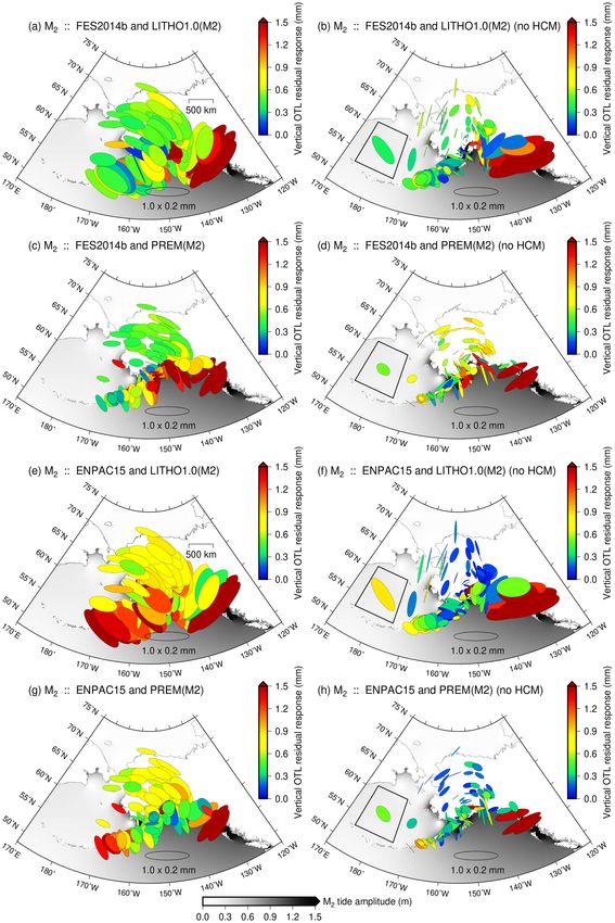
Figs 8 and 9 show selected residual displacements for the O1 and example, is effective at improving fits to the observed M2 displace-
Mf harmonics, respectively. We again compare combinations of the ments, as well as to the north and up components of the O1 tide. Re-
FES2014b and ENPAC15 ocean-tide models with anelastic PREM cent studies of anelastic dispersion at tidal periods also found misfit
and LITHO1.0 Earth models. Removing a harmonic common mode reductions, but considered only the M2 harmonic (Bos et al. 2015;Ocean tidal loading in Alaska 465
Downloaded from https://academic.oup.com/gji/article-abstract/223/1/454/5863947 by California Institute of Technology user on 21 July 2020
Figure 7. Comparisons of M2 OTL residuals for four Earth- and tide-model combinations. The vector differences are shown by PMEs (see description in
Fig. 2 caption). Residuals are shown both before (left-hand column) and after (right-hand column) a harmonic common mode (HCM) has been estimated and
removed from the residuals. When a HCM has been removed, it is shown as a boxed PME in the lower left-hand corner of the figure. We consider the following
model combinations: FES2014b and anelastic LITHO1.0 (a and b); FES2014b and anelastic PREM (c and d); ENPAC15 and anelastic LITHO1.0 (e and f);
and ENPAC15 and anelastic PREM (g and h). The first panel in each pair (i.e. panels a, c, e and g) represents the residuals before the HCM is removed. The
second panel in each pair (i.e. panels b, d, f and h) represents the residuals after the HCM is removed.466 H.R. Martens and M. Simons
Downloaded from https://academic.oup.com/gji/article-abstract/223/1/454/5863947 by California Institute of Technology user on 21 July 2020
Figure 8. Same as Fig. 7, but for the O1 tidal harmonic. The Earth models have been adjusted to account for anelastic dispersion at the O1 tidal period.
Wang et al. 2020). Predictions of Mf OTL displacements are mostly anelastic dispersion (Fig. 6). We find that the regionally customized
insensitive to the choice of Earth model as well as to adjustments LITHO1.0 model yields relatively good fits to the observed vertical-
for anelastic dispersion (at the level of microns). The east com- component data, albeit poorer fits to the horizontal components of
ponent of the O1 tide exhibits larger residuals after correcting for the M2 and O1 tides.Ocean tidal loading in Alaska 467
Downloaded from https://academic.oup.com/gji/article-abstract/223/1/454/5863947 by California Institute of Technology user on 21 July 2020
Figure 9. Same as Fig. 7, but for the Mf tidal harmonic. The Earth models have been adjusted to account for anelastic dispersion at the Mf tidal period.
Although predicted and GPS-observed OTL displacements for adjacent to large-amplitude tides (e.g. Fig. 7). Coastal stations are
the M2 , O1 and Mf tides generally match at the level of 1 mm or highly sensitive to the details of the ocean-tide model due to their
better across Alaska regardless of the choice of ocean-tide or Earth proximity to the load (e.g. Martens et al. 2016a). Adopting a high-
model (Figs 5 and 6), larger residuals are found at coastal stations resolution regional model for the ocean tides, ENPAC15, helps to468 H.R. Martens and M. Simons
reduce the observational residuals for the up component of the M2 REFERENCES
harmonic (up to several mm) and the north component of the Mf Agnew, D.C., 2015. Earth tides, in Treatise on Geophysics, 2nd edn, Vol. 3,
harmonic (up to 0.1–0.2 mm), but not for all components and har- pp. 151–178, ed. Schubert, G., Elsevier B.V.
monics (Fig. 6). On the whole, the FES2014b model performs well Alterman, Z., Jarosch, H. & Pekeris, C., 1959. Oscillations of the Earth,
Proc. R. Soc. Lond., A, 252(1268), 80–95.
across all spatial components and tidal harmonics. The TPXO9-
Amante, C. & Eakins, B.W., 2009. ETOPO1 1 arc-minute global relief
Atlas model also provides relatively good fits to the observed data
model: procedures, data sources and analysis, NOAA Technical Memo-
for the M2 harmonic. For the relatively small Mf tide, the residu- randum NESDIS NGDC-24, National Geophysical Data Center, Marine
als reveal subtle, yet potentially detectable, discrepancies based on Geology and Geophysics Division, Boulder, Colorado.
choice of ocean-tide model of about 0.1–0.2 mm (same order of Aster, R.C., Borchers, B. & Thurber, C.H., 2013. Parameter Estimation and
Downloaded from https://academic.oup.com/gji/article-abstract/223/1/454/5863947 by California Institute of Technology user on 21 July 2020
magnitude as observational uncertainties). Inverse Problems, Academic Press.
Vector differences between predicted and observed OTL dis- Baker, T., 1984. Tidal deformations of the Earth, Sci. Prog. Oxford, 69,
placements commonly exhibit some uniformity in amplitude and 197–233.
phase across the network. To better characterize regional spatial Baker, T., Curtis, D. & Dodson, A., 1996. A new test of Earth tide models
variations in OTL response, we experiment with isolating and re- in central Europe, Geophys. Res. Lett., 23(24), 3559–3562.
Bar-Sever, Y.E., Kroger, P.M. & Borjesson, J.A., 1998. Estimating horizon-
moving a harmonic common mode from the residual OTL dis-
tal gradients of tropospheric path delay with a single GPS receiver, J.
placements, which likely arises in part from long-wavelength er-
geophys. Res., 103(B3), 5019–5035.
rors associated with GPS processing and ocean-tide modelling (cf. Bertiger, W., Desai, S.D., Haines, B., Harvey, N., Moore, A.W., Owen, S. &
Martens et al. 2016b). After removing a harmonic common mode, Weiss, J.P., 2010. Single receiver phase ambiguity resolution with GPS
median discrepancies between predicted (ENPAC15 and anelas- data, J. Geod., 84(5), 327–337.
tic PREM) and observed OTL displacements are only 0.3 mm Blewitt, G., 2003. Self-consistency in reference frames, geocenter definition,
or less across all three spatial components and tidal-frequency and surface loading of the solid Earth, J. geophys. Res., 108(B2), 2103.
bands (Figs 7–9h), which is close to the current limit of obser- Boehm, J., Werl, B. & Schuh, H., 2006. Troposphere mapping functions
vational precision. Furthermore, the residuals reveal consistent for GPS and very long baseline interferometry from European Centre for
spatial patterns, particularly for the M2 and O1 tides, that likely Medium-Range Weather Forecasts operational analysis data, J. geophys.
Res., 111(B2), doi:10.1029/2005JB003629.
contain important information about local and regional incon-
Bos, M.S., Penna, N.T., Baker, T.F. & Clarke, P.J., 2015. Ocean tide loading
sistencies with the assumed Earth structure and ocean-tide dis-
displacements in western Europe. Part 2: GPS-observed anelastic disper-
tribution, including deviations from spherically symmetric Earth sion in the asthenosphere, J. geophys. Res., 120(9), 6540–6557.
structure. Carrère, L., Lyard, F., Cancet, M., Guillot, A. & Roblou, L., 2012. FES2012:
a new global tidal model taking taking advantage of nearly 20 years of
altimetry, in Proceedings of meeting “20 Years of Altimetry”, Venice.
Cartwright, D. & Edden, A., 1973. Corrected tables of tidal harmonics,
AC K N OW L E D G E M E N T S Geophys. J. R. astr. Soc., 33, 253–264.
The LoadDef software used to model load-induced deformation is Cartwright, D. & Taylor, R., 1971. New computations of the tide-generating
available from Martens et al. (2019). Observed and predicted load- potential, Geophys. J. R. astr. Soc., 23, 45–74.
Dahlen, F. & Tromp, J., 1998. Theoretical Global Seismology, Princeton
tide displacements for the Alaska PBO network (computed here) are
Univ. Press.
provided in the Supporting Information. FES2014 was produced by
Darwin, G.H., 1898. The Tides and Kindred Phenomena in the Solar System:
Noveltis, Legos, and CLS and distributed by Aviso+, with sup- The Substance of Lectures Delivered in 1897 at the Lowell Institute,
port from CNES (https://www.aviso.altimetry.fr/). Fig- Boston, Massachusetts, Houghton, Mifflin, & Company.
ures were created using the Generic Mapping Tools (Wessel et al. Dziewonski, A.M. & Anderson, D.L., 1981. Preliminary reference Earth
2013) and Matplotlib (Hunter et al. 2007). GPS data used in our model, Phys. Earth Planet. Inter., 25(4), 297–356.
study are available in open archives from UNAVCO (ftp://data- Egbert, G.D. & Erofeeva, S.Y., 2002. Efficient inverse modeling of
out.unavco.org/pub/rinex/obs). HRM processed the GPS data, per- barotropic ocean tides, J. Atmos. Oceanic Technol., 19(2), 183–204.
formed the tidal harmonic analysis, generated the forward models Egbert, G.D., Erofeeva, S.Y. & Ray, R.D., 2010. Assimilation of altime-
of predicted tidal displacements, assessed uncertainties and residu- try data for nonlinear shallow-water tides: quarter-diurnal tides of the
Northwest European Shelf, Cont. Shelf Res., 30(6), 668–679.
als, produced the figures, and wrote the manuscript. MS provided
Farrell, W., 1972a. Deformation of the Earth by surface loads, Rev. Geophys.,
important feedback on the interpretation of results and the written
10(3), 761–797.
manuscript. HRM wishes to thank colleagues and staff at ETH- Farrell, W., 1972b. Global calculations of tidal loading, Nature, 238(81),
Zürich for their kind hospitality and engaging discussions during the 43–44.
summer and fall of 2019. We are grateful to two anonymous review- Foreman, M., 1977. Manual for tidal heights analysis and prediction, Pacific
ers for their constructive and thorough reviews of the manuscript. Mar. Sci. Rep., 77-10, 1–58.
We also extend a special thanks to Editor Duncan Agnew for his Foreman, M., Cherniawsky, J. & Ballantyne, V., 2009. Versatile harmonic
thoughtful reviews and fruitful discussions on tidal harmonic anal- tidal analysis: improvements and applications, J. Atmos. Oceanic Technol.,
ysis, as well as to Luis Rivera (Université de Strasbourg) for his 26(4), 806–817.
generous contributions to the load-tide modelling and interpreta- Fu, Y. & Freymueller, J.T., 2013. Repeated large slow slip events at the
southcentral Alaska subduction zone, Earth planet. Sci. Lett., 375, 303–
tion of results. This material is based on work supported by the
311.
National Science Foundation under Grant No. 1925267 and the
Fu, Y., Freymueller, J.T. & van Dam, T., 2012. The effect of using inconsistent
National Aeronautics and Space Administration under Grant No. ocean tidal loading models on GPS coordinate solutions, J. Geod., 86(6),
NNX15AK40A. This material is also based on services provided 409–421.
by the GAGE Facility, operated by UNAVCO, Inc., with support Godin, G., 1972. The Analysis of Tides, University of Toronto Press.
from the National Science Foundation and the National Aeronau- Guo, J., Li, Y., Huang, Y., Deng, H., Xu, S. & Ning, J., 2004. Green’s
tics and Space Administration under NSF Cooperative Agreement function of the deformation of the Earth as a result of atmospheric loading,
EAR-11261833. Geophys. J. Int., 159(1), 53–68.You can also read