A daily, 250 m and real-time gross primary productivity product (2000-present) covering the contiguous United States - ESSD
←
→
Page content transcription
If your browser does not render page correctly, please read the page content below
Earth Syst. Sci. Data, 13, 281–298, 2021
https://doi.org/10.5194/essd-13-281-2021
© Author(s) 2021. This work is distributed under
the Creative Commons Attribution 4.0 License.

         A daily, 250 m and real-time gross primary productivity
                   product (2000–present) covering the
                        contiguous United States
             Chongya Jiang1,2,3 , Kaiyu Guan1,2,3,4 , Genghong Wu1,2,3 , Bin Peng1,3,4 , and Sheng Wang1,2,4
               1 Agroecosystem     Sustainability Center, Institute for Sustainability, Energy, and Environment,
                             University of Illinois at Urbana-Champaign, Urbana, IL 61801, USA
        2 College of Agricultural, Consumer & Environmental Sciences, University of Illinois at Urbana-Champaign,

                                                     Urbana, IL 61801, USA
                  3 DOE Center for Advanced Bioenergy and Bioproducts Innovation, University of Illinois at

                                         Urbana-Champaign, Urbana, IL 61801, USA
               4 National Center for Supercomputing Applications, University of Illinois at Urbana-Champaign,

                                                     Urbana, IL 61801, USA
         Correspondence: Chongya Jiang (chongya.jiang@email.com) and Kaiyu Guan (kaiyuguan@gmail.com)

                                 Received: 14 February 2020 – Discussion started: 25 May 2020
                     Revised: 4 November 2020 – Accepted: 11 November 2020 – Published: 9 February 2021

      Abstract. Gross primary productivity (GPP) quantifies the amount of carbon dioxide (CO2 ) fixed by plants
      through photosynthesis. Although as a key quantity of terrestrial ecosystems, there is a lack of high-spatial-
      and-temporal-resolution, real-time and observation-based GPP products. To address this critical gap, here we
      leverage a state-of-the-art vegetation index, near-infrared reflectance of vegetation (NIRV ), along with accu-
      rate photosynthetically active radiation (PAR), to produce a SatelLite Only Photosynthesis Estimation (SLOPE)
      GPP product for the contiguous United States (CONUS). Compared to existing GPP products, the proposed
      SLOPE product is advanced in its spatial resolution (250 m versus >500 m), temporal resolution (daily ver-
      sus 8 d), instantaneity (latency of 1 d versus >2 weeks) and quantitative uncertainty (on a per-pixel and daily
      basis versus no uncertainty information available). These characteristics are achieved because of several tech-
      nical innovations employed in this study: (1) SLOPE couples machine learning models with MODIS atmo-
      sphere and land products to accurately estimate PAR. (2) SLOPE couples highly efficient and pragmatic gap-
      filling and filtering algorithms with surface reflectance acquired by both Terra and Aqua MODIS satellites
      to derive a soil-adjusted NIRV (SANIRV ) dataset. (3) SLOPE couples a temporal pattern recognition ap-
      proach with a long-term Cropland Data Layer (CDL) product to predict dynamic C4 crop fraction. Through
      developing a parsimonious model with only two slope parameters, the proposed SLOPE product explains
      85 % of the spatial and temporal variations in GPP acquired from 49 AmeriFlux eddy-covariance sites (324
      site years), with a root-mean-square error (RMSE) of 1.63 gC m−2 d−1 . The median R 2 over C3 and C4
      crop sites reaches 0.87 and 0.94, respectively, indicating great potentials for monitoring crops, in particu-
      lar bioenergy crops, at the field level. With such a satisfactory performance and its distinct characteristics
      in spatiotemporal resolution and instantaneity, the proposed SLOPE GPP product is promising for biologi-
      cal and environmental research, carbon cycle research, and a broad range of real-time applications at the re-
      gional scale. The archived dataset is available at https://doi.org/10.3334/ORNLDAAC/1786 (download page:
      https://daac.ornl.gov/daacdata/cms/SLOPE_GPP_CONUS/data/, last access: 20 January 2021) (Jiang and Guan,
      2020), and the real-time dataset is available upon request.

Published by Copernicus Publications.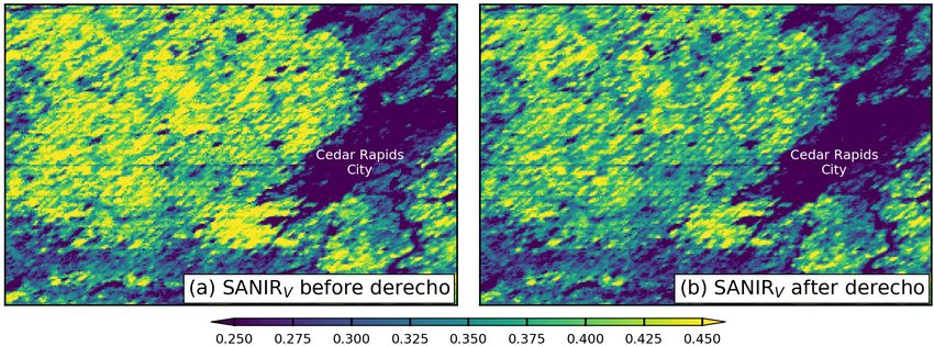
282                                                                                       C. Jiang et al.: SLOPE GPP product

1   Introduction                                                   but retrieved by complicated algorithms, and their accuracy
                                                                   still needs significant improvement to meet requirements of
Gross primary productivity (GPP) quantifies the amount of          Earth system models (GCOS, 2011).
carbon dioxide (CO2 ) fixed by plants through photosynthe-            Alternative approaches which heavily rely on reliable
sis (Beer et al., 2010; Jung et al., 2017). Because GPP is         satellite observations with low dependence on uncertain
the largest carbon flux and influences other ecosystem pro-        model structure or parameterization and model inputs are
cesses such as respiration and transpiration, monitoring GPP       highly required. Solar-induced fluorescence (SIF) emerged
is crucial for understanding the global carbon budget and          in recent years and may provide a new opportunity for GPP
terrestrial-ecosystem dynamics (Bonan, 2019; Friedlingstein        estimation (Guanter et al., 2014). Linear relationships have
et al., 2019). In addition, biomass accumulation driven by         been found between SIF and GPP at various ecosystems (Liu
GPP is the basis for food, feed, wood and fiber production,        et al., 2017; Magney et al., 2019; Yang et al., 2015). How-
and therefore monitoring GPP is crucial for human welfare          ever, satellite SIF data generally have coarse resolution, large
and development (Guan et al., 2016; Ryu et al., 2019).             spatial gaps, short temporal coverage and limited quality (Ba-
   Over the past 2 decades, a number of GPP products with          cour et al., 2019; Zhang et al., 2018) and are therefore not
different spatial and temporal characteristics have been de-       suitable for many applications.
rived using remote sensing approaches (Xiao et al., 2019).            Near-infrared reflectance of vegetation (NIRV,Ref ), de-
However, since GPP cannot be directly observed at large            fined as the product of the normalized difference vegeta-
scales, different models have been developed and used in           tion index (NDVI) and observed NIR reflectance (NIRRef )
generating GPP products. Process-based models use a se-            (Eq. 1), has recently been presented as a proxy of GPP (Bad-
ries of nonlinear equations to represent the atmosphere–           gley et al., 2017). A global monthly 0.5◦ GPP dataset has
vegetation–soil system and associated fluxes. For example,         been produced from satellite data using the linear relation-
a publicly available global GPP product using process-based        ship between NIRV,Ref and GPP (Badgley et al., 2019), ex-
models is the Breathing Earth System Simulator (BESS)              plaining 68 % GPP variations observed by the FLUXNET
(Jiang and Ryu, 2016). Machine-learning models upscale             network. Several field studies have recently found that taking
site-observed GPP to a larger scale by establishing non-           incoming radiation into account further improves the NIRV –
parametric relationships between the ground truth and grid-        GPP relationship (Dechant et al., 2020; Wu et al., 2020).
ded explanatory variables. The FLUXCOM GPP product is              Because MODIS provides long-term and real-time (2000–
a typical example of this approach (Jung et al., 2019). Semi-      present) observations of red (RedRef ) and NIR (NIRRef )
empirical approaches utilize equations with a concise physio-      reflectance and atmospheric conditions with high spatial
logical meaning (e.g., light use efficiency) that are parameter-   (250 m for reflectance and 1 km for atmosphere) and tem-
ized with several empirical constraint functions. The MOD17        poral (daily) resolutions, now there is an unprecedented op-
(MODIS GPP/NPP – net primary production – Project) GPP             portunity to generate an observation-based GPP product.
product (Running et al., 2004), the Vegetation Photosynthe-
                                                                                                  NIRRef − RedRef
sis Model (VPM) GPP product (Zhang et al., 2017) and the           NIRV,Ref = NDVI × NIRRef =                     × NIRRef (1)
Global LAnd Surface Satellite (GLASS) GPP product (Yuan                                           NIRRef + RedRef
et al., 2010) belong to this category.                                Leveraging the concept of NIRV , here we present a new
   With differing principles, assumptions and complexity, ex-      GPP model and the resultant daily, 250 m and real-time
isting remote sensing GPP models heavily rely upon inputs          GPP product (2000–present) covering the contiguous United
with large uncertainties. First, climate forcing, such as tem-     States (CONUS) (Jiang and Guan, 2020). The product is
perature, humidity, precipitation and wind speed, is com-          named SatelLite Only Photosynthesis Estimation (SLOPE)
monly used in these GPP models. However, these meteo-              because (1) the model only uses satellite data and (2) the
rological data are not observed but derived from reanaly-          model only has two slope parameters. Detailed model de-
sis approaches and usually have coarse spatial resolution          sign, multi-source satellite data processing and comprehen-
(e.g., >10 km) and large time lags (e.g., weeks). Second,          sive evaluation procedures are elucidated below.
plant functional types (PFTs) are used to define different
parameterization schemes in those models. To date, satel-
                                                                   2   Production of the SLOPE product
lite land cover products are usually characterized by con-
siderably large time lags (>1 year), relatively low accuracy
                                                                   The method we used to estimate GPP using the novel veg-
(≤ 70 %) (Yang et al., 2017) and more uncertainties with re-
                                                                   etation index NIRV,Ref follows the concept of light use effi-
gards to year-to-year variations (Cai et al., 2014; Li et al.,
                                                                   ciency (LUE) (Monteith, 1972; Monteith and Moss, 1977):
2018). Third, high-level remote sensing land products such
as the leaf area index (LAI), fraction of absorbed photosyn-       GPP = PAR × FPAR × LUE.                                     (2)
thetically active radiation (FPAR), clumping index (CI), land
surface temperature (LST) and soil moisture (SM) are used            Since NIRV,Ref has been found strongly correlated to
by some models. These variables are not directly observed          FPAR (Badgley et al., 2017) and moderately correlated to

Earth Syst. Sci. Data, 13, 281–298, 2021                                            https://doi.org/10.5194/essd-13-281-2021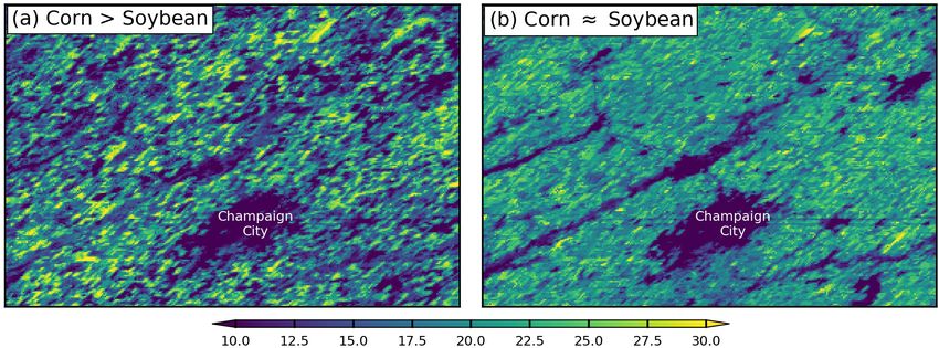
C. Jiang et al.: SLOPE GPP product                                                                                          283

LUE (Dechant et al., 2019), it is possible to simplify Eq. (2)     1fC4 , 1PAR and 1SANIRV ), the uncertainty of GPP can
as                                                                 be estimated in a spatiotemporally explicit manner by

GPP ≈ PAR × a × NIRV,Ref + b ,                             (3)     1GPP = (fC4 × PAR × SANIRV ) × 1cC4

                                                                        + (1 − fC4 ) × PAR × SANIRV 1cC3
where a and b are the slope and intercept, which can be fitted          + [(cC4 − cC3 ) × PAR × SANIRV ] 1fC4
from ground GPP observations. Both PAR (photosyntheti-
                                                                        + cC4 × fC4 + cC3 × (1 − fC4 ) × SANIRV 1PAR
cally active radiation) and NIRV,Ref can be easily derived
from satellite observations with high spatial and temporal              + cC4 × fC4 + cC3 × (1 − fC4 ) × PAR 1SANIRV .        (8)
resolutions in real time, avoiding complicated but uncertain
algorithm or parameterization to quantify FPAR and LUE in
Eq. (2). This linear relationship is likely to converge within
C3 species (Badgley et al., 2019) but differs between C3 and       2.1   Derivation of PAR
C4 species (Wu et al., 2019). Accordingly, land cover data         SLOPE adopts several machine learning approaches to com-
with considerably large time lags and relatively low accu-         pute PAR using forcing data mainly from Terra and Aqua
racy may not be necessary for the model parameterization.          MODIS Atmosphere and Land products (data solely from
Instead, an in-season C3–C4 species dataset is needed for          morning satellite Terra, afternoon satellite Aqua and com-
the accurate calibration of the linear relationship.               bination of the two satellites are called MOD, MYD and
   Defining the ratio of GPP to PAR as the incident PAR use        MCD, respectively, hereinafter). The list of inputs includes
efficiency (iPUE) gives                                            aerosol optical depth (AOD) at 3 km resolution from the
                                                                   MOD04_3K (MODIS/Terra Aerosol 5Min L2 Swath 3km)
iPUE = GPP/PAR = FPAR × LUE ≈ a × NIRV,Ref + b. (4)
                                                                   and MYD04_3K (MODIS/Aqua Aerosol 5Min L2 Swath
   Here iPUE is a confounding factor of canopy structure and       3km) products (Remer et al., 2013), total column wa-
leaf physiology, representing the capacity of plants to use in-    ter vapor (TWV) at 1 km resolution from the MOD05_L2
coming radiation for photosynthesis. When vegetation is ab-        (MODIS/Terra Total Precipitable Water Vapor 5-Min L2
sent, iPUE is zero and NIRV,Ref is expected to be zero too.        Swath 1km and 5km) and MYD05_L2 (MODIS/Aqua To-
However, this is not true in reality, as >99.9 % soils have        tal Precipitable Water Vapor 5-Min L2 Swath 1km and 5km)
positive NIRV,Ref values according to a global soil spectral li-   products (Chang et al., 2015), cloud optical thickness (COT)
brary (Jiang and Fang, 2019), and the correction of NIRV,Ref       at 1 km resolution from the MOD06_L2 (MODIS/Terra
for soil is needed for better performance at low vegetation        Clouds 5-Min L2 Swath 1km and 5km) and MYD06_L2
cover (Zeng et al., 2019). To address this issue, we will pro-     (MODIS/Aqua Clouds 5-Min L2 Swath 1km and 5km) prod-
pose a spatially explicit correction for NIRV,Ref to derive a      ucts (Baum et al., 2012), total column ozone burden (TO3) at
soil-adjusted index SANIRV (see details in Sect. 2.2). Since       5 km resolution from the MOD07_L2 (MODIS/Terra Tem-
SANIRV = 0 when iPUE = 0, Eq. (4) becomes                          perature and Water Vapor Profiles 5-Min L2 Swath 5km) and
                                                                   MYD07_L2 (MODIS/Aqua Temperature and Water Vapor
iPUE ≈ c × SANIRV ,                                         (5)    Profiles 5-Min L2 Swath 5km) products (Borbas et al., 2015),
                                                                   white-sky land surface shortwave albedo (ALB) at 500 m res-
where c is the slope coefficient.                                  olution from the MCD43A3 (MODIS/Terra+Aqua Albedo
  Considering the presence of mixed pixels of C3 and C4            Daily L3 Global 500m SIN Grid) product (Román et al.,
species with the 250 m pixels, Eq. (5) can be rewritten as         2009), and altitude (ALT) at 30 m resolution from the Shuttle
                                                                 Radar Topography Mission Global 1 arc second (SRTMGL1)
iPUE ≈ cC4 × fC4 + cC3 × (1 − fC4 ) × SANIRV ,             (6)     product (Kobrick and Crippen, 2017).
                                                                      MODIS atmosphere products are swath data, and swaths
where cC4 and cC3 are the coefficients for C4 and C3 species,
                                                                   vary day by day. To maintain consistency and facilitate fur-
respectively, and fC4 is the fraction of C4 species in vegeta-
                                                                   ther usage, all data are reprojected using the nearest neigh-
tion. Therefore, the SLOPE GPP model is
                                                                   bor resampling approach to the Conus Albers projection on

GPP ≈ cC4 × fC4 + cC3 × (1 − fC4 ) × PAR × SANIRV . (7)            the North American Datum of 1983 (NAD83) (European
                                                                   Petroleum Survey Group – EPSG:6350) with 1 km spatial
   In the SLOPE model (Eq. 7), PAR, SANIRV and fC4                 resolution. For swath data, an overlap area exists between
are remote sensing inputs, whereas cC4 and cC3 are model           two paths. In this case, data with smaller sensor view zenith
parameters to be calibrated using ground-truth GPP data            angles provided by MOD/MYD03_L2 products are chosen.
(Fig. 1). In the following sections, we will elaborate on the      MODIS land products and SRTMGL1 are tile data with
derivation of PAR, SANIRV and fC4 , along with their quanti-       finer resolution than 1 km. They are reprojected to the EPSG
tative uncertainties, and the model calibration for parameters     6350 spatial reference by aggregating all fine-resolution pix-
cC4 and cC3 . With the uncertainty of each term (1cC4 , 1cC3 ,     els within each 1 km grid.

https://doi.org/10.5194/essd-13-281-2021                                            Earth Syst. Sci. Data, 13, 281–298, 2021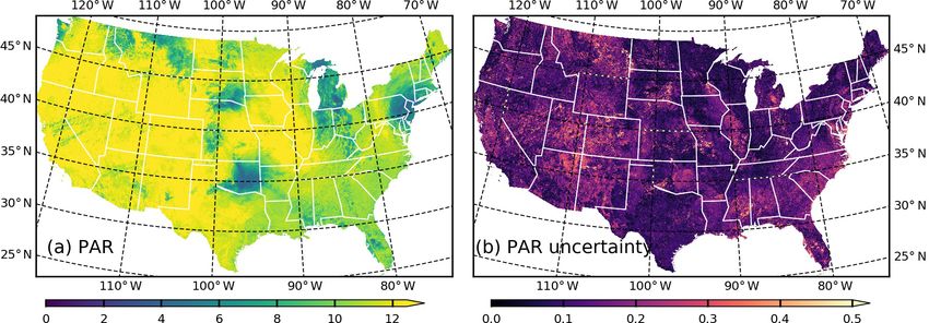
284                                                                                         C. Jiang et al.: SLOPE GPP product

Figure 1. Framework to produce the SLOPE GPP product. The box with dashed lines is the legend.

   Data gaps exist in all MODIS products, and a gap-filling         in addition to atmosphere data, whereas for pPAR , ALB, ALT
measure is required. For MODIS atmosphere products, gaps            and the estimated tSWR are used. A summary of model inputs
in MOD and MYD are first filled by data in the MYD and              is listed in Table 1.
MOD counterpart on the same day, followed by a multi-year              Four different machine learning approaches are em-
average on that day. Since the multi-year average of COT is         ployed to estimate tSWR and pPAR . They are the least ab-
always non-zero, directly using it for a gap-filling measure        solute shrinkage and selection operator (LASSO) (Tibshi-
always implies a cloudy condition. Therefore, a CLARA-2             rani, 1996), multivariate adaptive regression splines (MARS)
(cLoud, Albedo and surface Radiation) cloud mask at 0.05◦           (Friedman, 1991), k-nearest neighbor regression (KNN)
acquired from NOAA AVHRR (Advanced Very High Reso-                  (Goldberger et al., 2005), and random forest regression (RF)
lution Radiometer) data is employed (Karlsson et al., 2017).        (Liaw and Wiener, 2002). We used scikit-learn, a free soft-
Only MODIS data gaps for AVHRR cloudy pixels are filled             ware machine learning library for the Python programming
by a multi-year average of COT, whereas MODIS COT data              language to build the models. All the four algorithms were
gaps for AVHRR clear pixels are set to 0. For the MODIS             automatically optimized by tuning their hyperparameters us-
land product, i.e., ALB, a temporally moving window with a          ing 5-fold cross validation on their training dataset. All inputs
7 d radius is utilized for a specific day, and a Gaussian filter    and outputs are the same for the four approaches. Four differ-
is applied to the time series data within the moving window         ent PAR estimations are then obtained by Eq. (9), and their
on a per-pixel basis. The filtered values are used to fill gaps     ensemble mean and standard deviation are considered as the
on that specific day.                                               final estimation and uncertainty, respectively.
   Machine learning approaches are used to upscale the
ground truth to satellite data. The ground truth is from the        PAR = SWRTOA × tSWR × pPAR                                   (9)
Surface Radiation Budget (SURFRAD) Network (Augus-
tine et al., 2000), including seven long-term continuous sites      2.2   Derivation of SANIRV
across the CONUS. Daily-mean shortwave radiation (SWR)
and PAR on the surface are calculated from site observations        SLOPE derives NIRV,Ref (Eq. 1) from MODIS band 1 (red)
at 1–3 min intervals from 2000 through 2018. Daily-mean             and band 2 (NIR) surface reflectance (SR) at 250 m resolu-
top-of-atmosphere SWR (SWRTOA ) is calculated using lati-           tion from MOD/MYD09GQ products (Vermote et al., 2002).
tude and day-of-year (DOY) information (Allen et al., 1998).        Only pixels with quality control (QC) information defined as
Subsequently, atmospheric transmittance (tSWR ) and propor-         “corrected product produced at ideal quality all bands” were
tion of PAR in SW (pPAR ) are calculated as SWR / SWRTOA            used. Since cloud and cloud shadows substantially reduce
and PAR / SWR.                                                      NIRV,Ref values, SLOPE adopts three strategies to mitigate
   Models are built to estimate tSWR first, followed by pPAR .      the cloud contamination.
MOD data representing atmospheric conditions in the morn-              First, the cloud mask is applied. MOD–MYD COT data
ing and MYD for the afternoon are used separately for the           processed in Sect. 2.1 are resampled to the same spatial refer-
estimation, and the two estimates are averaged to account           ence with MOD–MYD SR data and used to mask out cloudy
for discrepancies between the morning and afternoon. Clear          pixels. At this point, a morphological dilation operation is
and cloudy conditions are also treated separately in modeling       used to enlarge the cloud mask to account for cloud edges.
considering the absence or presence of non-zero COT data.           However, since COT data have a coarser resolution (1 km)
For the estimation of tSWR , ALB, ALT and SWRTOA are used           than SR data (250 m), there are still partial clouds and cloud
                                                                    shadows left after this step.

Earth Syst. Sci. Data, 13, 281–298, 2021                                              https://doi.org/10.5194/essd-13-281-2021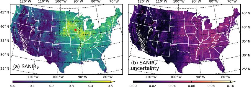
C. Jiang et al.: SLOPE GPP product                                                                                                  285

Table 1. Summary of machine learning model inputs for the estimation of tSWR and pPAR . Daily estimations from MOD and MYD atmo-
sphere data are averaged.

                            Inputs          For daily tSWR estimation                For daily pPAR estimation
                                            MOD                 MYD                  MOD                 MYD
                                       Clear   Cloudy     Clear       Cloudy    Clear   Cloudy      Clear   Cloudy
                                                 √                      √                 √                   √
                            log(COT)
                                        √        √          √           √        √        √          √        √
                            log(AOD)
                                        √        √          √           √        √        √          √        √
                            TWV
                                        √        √          √           √        √        √          √        √
                            TO3
                                        √        √          √           √        √        √          √        √
                            ALB
                                        √        √          √           √        √        √          √        √
                            ALT
                                        √        √          √           √
                            SWRTOA
                                                                                 √         √         √         √
                            tSWR

    Second, MOD and MYD data are combined. Ideally, on                       To minimize the effects of variations in soil brightness
a specific day, MOD and MYD NIRV,Ref should be identi-                    on NIRV,Ref , soil background NIRV (NIRV,Soil ) is identified
cal if they are obtained under the same conditions. However,              from multi-year average NIRV,Ref time series. For a spe-
the remaining cloud contamination and sun-target-sensor ge-               cific pixel, soil background NIRV (NIRV,Soil ) is supposed
ometry could cause differences between morning and after-                 to be (1) smaller than seasonal mean NIRV,Ref , which in-
noon observations. Considering that the vegetation index is               cludes the vegetated period, and (2) smaller than 0.2 indi-
more sensitive to cloud contamination than the sensor view                cated by a global soil spectral library (Jiang and Fang, 2019).
zenith angle, a simple criterion is applied to combine MOD                Therefore, NIRV,Soil is supposed to within a range of [0,
and MYD observations. If the difference between MOD and                   min(mean(NIRV,Ref ), 0.2)]. The mode of daily NIRV,Ref av-
MYD NIRV,Ref is greater than or equal to a predefined                     eraged over 2000–2019 within this value range is considered
threshold (0.1 in this study), then the smaller one is likely             as NIRV,Soil . An example is given in Fig. S5. Theoretically,
cloud contaminated, and the larger one is used. Otherwise,                NIRV,Soil for evergreen species cannot be obtained from time
the average value of the two is used. However, in many cases,             series NIRV,Ref because of the persistent vegetation cover.
both MOD and MYD data are contaminated, and the sensor                    Pixels with a NIRV,Soil value larger than 0.1 and seasonal
view zenith angle may cause unexpected day-to-day varia-                  coefficient of variation (CV) of NIRV,Ref smaller than 33 %
tions.                                                                    are empirically considered as evergreen species, and their
    Third, a temporal filter is applied. The filter is based on the       NIRV,Soil values are set to 0.
assumption that NIRV,Ref should change smoothly within a                     Finally, SANIRV is defined as
short time period. Accordingly, a temporally moving win-
dow with a 7 d radius is utilized for a specific day. The mean                          NIRV,Ref − NIRV,Soil
                                                                          SANIRV =                            × NIRV,Peak ,         (10)
and standard deviation are calculated from the NIRV,Ref                                 NIRV,Peak − NIRV,Soil
time series on a per-pixel basis. Values outside the range of
                                                                          where NIRV,Peak is the maximum value of the multi-
mean ±1.5 standard deviations are considered as outliers and
                                                                          year average NIRV,Ref time series on a per-pixel basis.
dropped. Subsequently, the mean of the first 3 d and that of
                                                                          SANIRV does not change NIRV,Peak but changes more
the last 7 d are calculated, respectively. If the NIRV,Ref value
                                                                          for low NIRV,Ref values. SANIRV,Ref is set to 0 when
of the target day is 20 % smaller or larger than both the first
                                                                          NIRV,Ref ≤ NIRV,Soil . In general, SANIRV is supposed to be
3 d mean and the last 3 d mean, then that NIRV,Ref value is
                                                                          smooth within a short time period; therefore, the standard
considered as an outlier and dropped.
                                                                          deviation within the ±3 d temporal window is calculated as
    After the removal of outliers, a large amount of data gaps
                                                                          uncertainty.
exist, and a gap-filling measure is required. Similar to ALB
in Sect. 2.1, a temporally moving window with a 7 d radius
is utilized for a specific day, and a Gaussian filter is applied          2.3   Derivation of the C4 fraction
and used to fill gaps on that day. The rest of the data gaps are          A National Land Cover Database (NLCD) along with a crop-
filled with the multi-year average of NIRV,Ref . Considering              specific land cover product Cropland Data Layer (CDL)
extreme cases for which no data are available on a specific               are used to derive the fraction cover of C4 crop in vegeta-
day over all years, the multi-year average of ±3 d is used for            tion (fC4 ). NLCD is a comprehensive land cover database
the final gap-filling measure.                                            produced by the United States Geological Survey (USGS).
                                                                          It provides several main thematic classes such as urban,

https://doi.org/10.5194/essd-13-281-2021                                                       Earth Syst. Sci. Data, 13, 281–298, 2021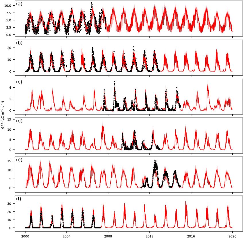
286                                                                                         C. Jiang et al.: SLOPE GPP product

agriculture and forest with high accuracy (Homer et al.,             2.4    Calibration for iPUE coefficients
2004). The 30 m nationwide NLCD data are available for
2001, 2004, 2006, 2008, 2011, 2013 and 2016. CDL is an               SLOPE was calibrated using the GPP data derived from
agriculture-oriented product produced by the United States           AmeriFlux site observations. The AmeriFlux network is a
Department of Agriculture (USDA). It provides >100 crop              community of sites that use eddy-covariance technology to
cover types and leverages other land cover types from NLCD           measure landscape-level carbon, water and energy fluxes
(Boryan et al., 2011). Across the CONUS CDL data are                 across the Americas (Baldocchi et al., 2001). A total of
available at a 30 m spatial resolution and in a yearly tem-          48 sites (324 site years) were involved in this study (Ta-
poral frequency from 2008 through 2019, whereas in some              ble S3). All of the 43 sites in the FLUXNET2015 Tier
areas annual data are available back to the 1990s.                   1 dataset (variable name: GPP_DT_VUT_MEAN; qual-
   The fraction of C4 crop in vegetated areas is first derived       ity control: NEE_VUT_REF_QC) in the CONUS were
using existing CDL data. NLCD land cover types are cat-              used because this dataset was produced by a standard-
egorized into vegetated areas and non-vegetated areas with           ized data processing pipeline with strict data quality con-
30 m resolution. The fraction of vegetated areas in total area       trol protocols and is commonly considered the ground truth.
is subsequently calculated for each 250 m pixel. Similarly,          Additionally, seven sites were from the AmeriFlux level
CDL crop types are categorized into C4-planted areas and             4 dataset (variable name: GPP_or_MDS; quality control:
non-C4 areas with 30 m resolution. The fraction of C4 crops          NEE_or_fMDSsqc). This dataset was generated more than
in total area is subsequently calculated for each 250 m pixel.       10 years ago, and only AmeriFlux Core Sites that are not
The ratio of the fraction of C4 crops in total area to the frac-     covered by FLUXNET2015 were used for data quality con-
tion of vegetated areas in total area is calculated to derive        sideration. For both datasets, only days with the best quality
the fraction of C4 crops in vegetated areas at 250 m resolu-         control flags were used in the SLOPE modeling and evalua-
tion. Since NLCD data are not available for every year, an           tion procedures.
assumption is made that 1 year of NLCD data can represent               We used Eq. (5) to conduct model calibration. Although
adjacent years. Specifically, NLCD 2001 is used for 2000–            SLOPE considers the iPUE–SANIRV relationship for C3 and
2002; NLCD 2004 is used for 2003 and 2004; NLCD 2006 is              C4 species, we also tested other configurations for compar-
used for 2005 and 2006; NLCD 2008 is used for 2007–2009;             ison purposes. Configuration 1 (“all”) is defined as follows:
NLCD 2011 is used for 2010 and 2011; NLCD 2013 is used               all data were used together to fit a universal iPUE coefficient
for 2012–2014; and NLCD 2016 is used for 2015–2019.                  c. Configuration 2 (“C3–C4”) is defined as follows: data were
   To predict the fraction of C4 crop in vegetation for re-          separated for C3 and C4 species to fit cC3 and cC4 , respec-
gion years for which no CDL data are available, crop rotation        tively. It is worth mentioning that only C4 crops (six sites)
patterns are identified from historical data. Assuming that C4       were considered as C4 species, whereas C4 grass and shrubs
crops are planted following three rotation strategies: C4–non-       (three sites: US-SRG, Santa Rita Grassland; US-SRM, Santa
C4, C4–C4–non-C4 and non-C4–non-C4–C4 and assigning                  Rita Mesquite; and US-Wkg, Walnut Gulch Kendall Grass-
1 to C4 and 0 to non-C4, a total of eight possible time se-          lands) were still categorized into C3 species because of the
ries during the period of 2008–2019 when nationwide CDL              lack of nationwide and high-resolution C4 grass and shrub
data are available are listed in Table 2. On a per-pixel basis,      data. Configuration 3 (“PFTs”) is defined as follows: data
the time series of the fraction of C4 crop in vegetation ar-         were separated for different PFTs, evergreen needleleaf for-
eas during 2008–2019 is compared with the eight predefined           est (ENF; 14 sites), deciduous broadleaf forest and mixed
rotation patterns. The Pearson coefficient r is calculated be-       forest (DBF and MF; 8 sites), shrubland and woody savannah
tween actual time series and each of the eight patterns, and         (SHR and WSA; 5 sites), grassland (GRA; 8 sites), wetland
the pattern yielding the largest r is the identified rotation pat-   (WET; 5 sites), C3 cropland (10 sites) and C4 cropland (6
tern. Once the pattern is identified, the fraction of C4 crop        sites), to fit PFT-specific iPUE coefficients. The RMSE be-
in vegetated areas in any unknown year can be inferred. If           tween SANIRV -derived and AmeriFlux iPUE for C3 and C4
1 year is inferred as C4, then the multi-year average of the         are calculated as uncertainties of cC3 and cC4 , respectively.
C4 fraction over C4-dominated years is used. Otherwise, the
multi-year average over C3-dominated years is used. If the           3     Evaluation of the SLOPE product
largest r is smaller than 0.497, i.e., p>0.1 for 12 years, then
it is considered as no significant pattern, and the multi-year       3.1    Performance of PAR
average over all years is used. The RMSE between the pre-
dicted and reference CDL C4 fraction is calculated as uncer-         SLOPE PAR demonstrates distinctive and detailed spatial
tainty. To account for the land cover change, the predicted          variations in the CONUS because of the large spatial vari-
C4 crop fraction is set to 0 in years when NLCD data are not         ations of atmospheric conditions (Fig. 2a). As an example,
classified as cropland. It is worth mentioning that C4 grass-        on 10 July 2020, large areas in New Jersey, Wisconsin, Okla-
land and shrubland are not considered in this study, as no           homa, South Dakota and Montana display significantly lower
nationwide high-resolution distribution data are available.          values than other areas, due to dominant impacts of clouds

Earth Syst. Sci. Data, 13, 281–298, 2021                                               https://doi.org/10.5194/essd-13-281-2021
C. Jiang et al.: SLOPE GPP product                                                                                                     287

Table 2. Predefined C4-planting patterns from 2008 through 2019. If the C4 crop dominates in a specific year, 1 is assigned. Otherwise, 0 is
assigned.

                  Year    Pattern 1    Pattern 2   Pattern 3   Pattern 4     Pattern 5   Pattern 6   Pattern 7   Pattern 8
                  2008        1           0            1           1             0          0           0           1
                  2009        0           1            1           0             1          0           1           0
                  2010        1           0            0           1             1          1           0           0
                  2011        0           1            1           1             0          0           0           1
                  2012        1           0            1           0             1          0           1           0
                  2013        0           1            0           1             1          1           0           0
                  2014        1           0            1           1             0          0           0           1
                  2015        0           1            1           0             1          0           1           0
                  2016        1           0            0           1             1          1           0           0
                  2017        0           1            1           1             0          0           0           1
                  2018        1           0            1           0             1          0           1           0
                  2019        0           1            0           1             1          1           0           0

(Fig. S1). Aerosol optical depth (Fig. S2), total water va-                ing season, remarkably high SANIRV values (∼ 0.5) from
por (Fig. S3) and total ozone burden (Fig. S4) also influence              the Corn Belt in the central US are observed. This area is
the amount of clear-sky PAR to some degree. For example,                   one of the most productive areas on Earth, producing more
the southeastern part of the CONUS shows more aerosol and                  than 30 % of global corn and soybean (Green et al., 2018).
thus lower PAR values than other cloud-free areas. In addi-                Forested areas in the eastern and western US are character-
tion to the total amount of PAR, SLOPE PAR also reveals                    ized by relatively high values (0.3–0.4) and medium values
variations in the ratio of PAR to SWR (Fig. S5). Despite a                 (0.2–0.3), respectively. Low values (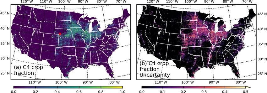
288                                                                                              C. Jiang et al.: SLOPE GPP product

Figure 2. Spatial distribution of 1 km resolution (a) PAR (MJ m−2 d−1 ) and (b) PAR uncertainty (MJ m−2 d−1 ) on 10 July 2020.

Figure 3. Comparison between site-observed PAR and SLOPE PAR. (a) Comparison across seven SURFRAD sites in 2019. (b) Comparison
across 41 AmeriFlux sites from 2000 to 2014. All site data are independent of the training procedure.

ber) seasonal pattern (Fig. 6d), which is caused by the pre-            located in the Corn Belt, especially in Indiana, Illinois, Iowa
cipitation seasonality there. The wetland site US-Myb (May-             and Nebraska. A direct comparison between the predicted C4
berry Wetland) is characterized by a long growing season                crop fraction (Fig. 8a) and independent reference CDL data
and a flat peak from April to November (Fig. 6e). The crop-             (Fig. 8b) indicates that the SLOPE prediction is able to re-
land site US-Bo1 (Bondville) has corn planted in 2019, and              construct the spatial patterns of the fraction of C4 crop in
it shows the highest SANIRV peak up to 0.5 among all the                vegetation at 250 m resolution. It is worth mentioning that
shown six sites (Fig. 6f). It is worth mentioning that com-             the uncertainty metric RMSE is sensitive to extreme values,
pared to the two raw satellite-observed NIRV values pro-                and it is different from the misclassification rate (0.4 does
vided by MOD09GQ and MYD09GQ products, respectively,                    not mean 40 %). For a pure pixel of a corn–soybean rotation
SLOPE SANIRV successfully removes the soil impact in the                field, the RMSE equals 0.39 if 3 out of 20 years are mis-
non-growing season as the values equal to or close to 0. In             classified, i.e., misclassification rate of 0.15. A further inves-
addition, SLOPE SANIRV is gap-free and much less con-                   tigation with regard to interannual dynamics shows that the
taminated by noises. Furthermore, spatiotemporally explicit             SLOPE predictions can even perform better than CDL refer-
uncertainty is associated with each SANIRV value.                       ence data (Fig. 9), benchmarked with the ground truth col-
                                                                        lected in the field. At this point, the CDL land cover could be
                                                                        prone to uncertainties in both satellite observation and clas-
3.3   Performance of the C4 fraction                                    sification algorithm, and classification is conducted year by
SLOPE predicts a reasonable fraction of the C4 crop in veg-             year without an interannual consideration (Lark et al., 2017).
etation in the CONUS (Fig. 7a). Most of the C4 crops are                SLOPE employs a rotation model to match decadal time se-

Earth Syst. Sci. Data, 13, 281–298, 2021                                                   https://doi.org/10.5194/essd-13-281-2021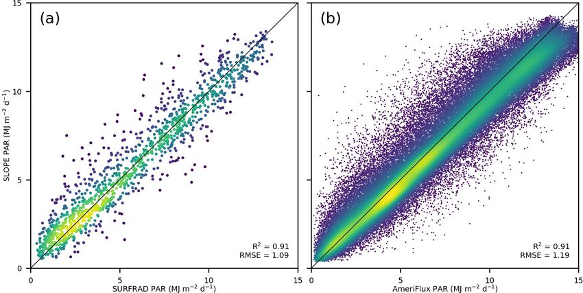
C. Jiang et al.: SLOPE GPP product 289
Figure 4. Spatial distribution of 250 m resolution (a) SANIRV and (b) SANIRV uncertainty across the CONUS on 10 July 2020.
Figure 5. SANIRV in a 50 × 75 km2 area at Cedar Rapids, Iowa (red marker in Fig. 4a), on (a) 9 Aug 2020 and (b) 13 Aug 2020. A severe
derecho took place from 10–11 August 2020. The maps are shown with the sinusoidal projection.
ries of CDL data, during which procedure noises in CDL timescales (Badgley et al., 2019; Chabot and Hicks, 1982).
data are suppressed. The features for which SLOPE is able Previous studies found that changes in the xanthophyll cy-
to reconstruct spatial and interannual patterns of CDL data cle instead of chlorophyll concentration or absorbed PAR
enable producing GPP in years when CDL data are unavail- explained the seasonal variation of photosynthetic capacity
able (e.g., 2020 and years before 2008 for most regions). It in evergreen needleleaf forest (Gamon et al., 2016; Magney
is worth mentioning that uncertainty is also associated with et al., 2019). Therefore, SIF was suggested by some studies
each pixel (Fig. 7b). as a better proxy of photosynthetic capacity in this ecosys-
tem (Smith et al., 2018; Turner et al., 2020), though satellite
SIF has coarser spatial resolution, shorter temporal coverage,
3.4 Performance of GPP
larger temporal latency and a lower signal-to-noise ratio than
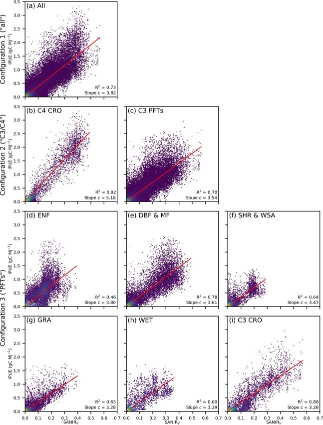
SLOPE SANIRV shows a strong linear correlation with iPUE SANIRV . In addition, the relatively weak iPUE–SANIRV re-
(Fig. 10). When data from all 49 sites (324 site years) are lationship is also partly because of the small value ranges in
used together, the SANIRV –iPUE relationship has an over- both SANIRV and iPUE.
all R 2 value of 0.73 (Fig. 10a). This is composed of an R 2 The overall slope is 3.82 gC MJ−1 for all data (Fig. 10a).
value of 0.92 from C4 species (Fig. 10b) and 0.70 from C3 A distinct difference is found between C4 (5.18; Fig. 10b)
species (Fig. 10c). C3 species can be further decomposed and C3 (3.54; Fig. 10c) species, suggesting the importance of
into six PFTs (Fig. 10d–i), among which cropland has the separating C4 from C3 species in modeling. The slope values
highest R 2 value up to 0.80 (Fig. 10i), whereas evergreen vary to a limited degree within C3 species (Fig. 10d–i), rang-
needleleaf forest has the lowest value of 0.46 (Fig. 10d). This ing from 3.26 gC MJ−1 (cropland; Fig. 10i) to 3.80 gC MJ−1
relatively weak iPUE–SANIRV relationship is expected be- (evergreen needleleaf forest; Fig. 10d), indicating the in-
cause evergreen needleleaf forest tends to allocate resources significance of separating different PFTs. It is worth men-
for leaf construction and maintenance at large timescales and tioning that the SANIRV –iPUE relationship has a zero inter-
does not have much flexibility to change canopy structure cept because of the successful removal of the soil impact.
and leaf color as a response to varying environment at small
https://doi.org/10.5194/essd-13-281-2021 Earth Syst. Sci. Data, 13, 281–298, 2021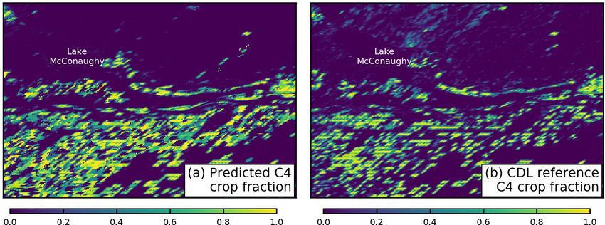
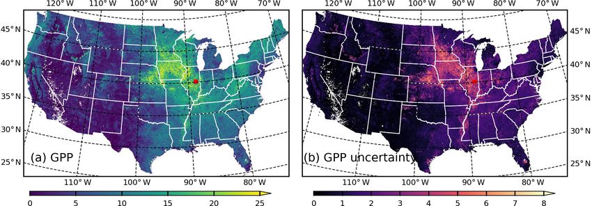
290                                                                                                C. Jiang et al.: SLOPE GPP product

Figure 6. Comparison between SANIRV and raw NIRV derived from MOD09GQ and MYD09GQ products at six AmeriFlux sites (Table S3)
in 2019. (a) US-Blo (evergreen needleleaf forest, ENF). (b) US-Ha1 (deciduous broadleaf forest, DBF). (c) US-Whs (open shrubland, OSH).
(d) US-AR1 (grassland, GRA). (e) US-Myb (wetland, WET). (f) US-Bo1 (cropland, CRO). Shaded areas indicate uncertainties of SANIRV .

Figure 7. Spatial distribution of 250 m resolution (a) predicted fraction of C4 crop in vegetation in 2000 and (b) C4 crop fraction uncertainty
across the CONUS.

   A 100-time-repeated 5-fold cross validation reveals the ro-               SLOPE GPP demonstrates detailed and distinctive spa-
bustness of the SANIRV –iPUE relationships (Fig. 11). Here                tial variations in the CONUS (Fig. 12a). The Corn Belt is
the repeated cross validation means the whole GPP dataset                 the most productive area, largely contributed by the C4 crop
from all 49 sites (324 site years) is randomly split into five            corn whose GPP could reach up to 30 gC m−2 d−1 (Fig. 13a).
folds, four folds for training and one fold for testing, and the          Forested areas in the eastern US show medium GPP val-
process is repeated 100 times yielding 500 training–testing               ues, followed by forests and croplands in the western US.
splits in total. In all subsets, the uncertainties of the iPUE            Grasslands and shrublands in the central and western US
coefficient c (the slope of the SANIRV –iPUE relationship)                generally show low productivity. On this example day, the
are less than 1 % (Fig. 11a). When using the three differ-                R 2 of spatial patterns between GPP and SANIRV , GPP and
ent model configurations, the model performances in sim-                  C4 fraction, and GPP and PAR across the CONUS are 0.89,
ulating the whole training–testing datasets also show little              0.34 and 0.01, respectively. SANIRV , an integrated vegeta-
variation (Fig. 11b), in general
C. Jiang et al.: SLOPE GPP product                                                                                                   291

Figure 8. C4 crop fraction of (a) SLOPE predicted and (b) CDL reference data in a 50 × 75 km2 area in Keith County, Nebraska (red marker
in Fig. 7a), in 2000. Only CDL data during 2008–2019 are used in the modeling procedure, and therefore (b) is independent of (a). The maps
are shown with the sinusoidal projection.

Figure 9. Comparison of fraction of C4 crop in vegetation between the field-collected ground truth, 250 m resolution CDL data and 250 m
resolution SLOPE predictions at six AmeriFlux sites (Table S3) in the US Corn Belt from 2000 to 2020. (a) US-Ne1 (uncertainty: 0.17; Mead
– irrigated continuous maize site). (b) US-Ne2 (uncertainty: 0.40; Mead – irrigated maize–soybean rotation site). (c) US-Ne3 (uncertainty:
0.18; Mead – rainfed maize–soybean rotation site). (d) US-Bo1 (uncertainty: 0; Bondville). (e) US-Ro1 (uncertainty: 0.16; Rosemount –
G21). Uncertainty is the RMSE between the predicted and the CDL reference.

fraction (Fig. 7a) because of smaller PAR values (Fig. 2a).            tial pattern shows that the Corn Belt has the largest uncer-
At a small scale (e.g., within a county), the 250 m resolu-            tainty (Fig. 12b; e.g., 5 gC m−2 d−1 ) due to the considerable
tion (∼ 0.06 km2 per pixel) SLOPE GPP is close to revealing            contribution from the uncertainty of the C4 fraction (Fig. 7b).
field-level heterogeneity, considering that the mean and me-              SLOPE GPP agrees fairly well with the ground truth from
dian crop field sizes in the CONUS are 0.19 and 0.28 km2 , re-         the AmeriFlux sites (Fig. 14). Across all of the 49 sites
spectively (Yan and Roy, 2016). For example, Fig. 13a shows            (328 site years; Fig. 14a), SLOPE GPP achieves an over-
large contrast in GPP, but Fig. 13b is more homogeneous.               all R 2 value of 0.85, RMSE of 1.63 gC m−2 d−1 and rela-
This is because corn reaches peak growing season in early              tive error of 37.8 %. For individual sites (Fig. 14b), the me-
July when soybean canopy is still open and sparse. SLOPE               dian R 2 and RMSE values are 0.80 and 1.69 gC m−2 d−1 ,
GPP with its pixel size much smaller than field area is there-         respectively. C4 cropland generally shows the highest me-
fore able to show GPP difference between corn and soybean.             dian R 2 value (0.94), followed by deciduous broadleaf for-
In late August, corn turns yellow, while soybean is still green        est and mixed forest (0.88) and C3 cropland (0.87). The
and active, and therefore they have similar GPP values con-            lowest median R 2 value (0.69) is observed for evergreen
sidering corn is C4, while soybean is C3. We suggest that              needleleaf forest. With regard to RMSE, smaller median
the 250 m resolution makes a big difference compared to ex-            values are found in grassland (1.09 gC m−2 d−1 ), shrub-
isting global GPP products whose spatial resolutions are at            land and woody savannah (1.48 gC m−2 d−1 ), and decidu-
least 500 m (∼ 0.25 km2 per pixel). Quantitative uncertainty           ous broadleaf forest and mixed forest (1.48 gC m−2 d−1 ),
is provided for each SLOPE GPP estimate (Eq. 8). The spa-

https://doi.org/10.5194/essd-13-281-2021                                                  Earth Syst. Sci. Data, 13, 281–298, 2021
292                                                                                              C. Jiang et al.: SLOPE GPP product

Figure 10. Comparison between SANIRV and iPUE over different subsets. The slope value of the SANIRV –iPUE relationship is the model
parameter c (Eq. 5). Panel (a) is used by the model configuration 1 (all). Panels (b) and (c) are used by the model configuration 2 (C3–C4),
which is actually used by SLOPE. Panels (b) and (d)–(i) are used by the model configuration 3 (PFTs).

Earth Syst. Sci. Data, 13, 281–298, 2021                                                   https://doi.org/10.5194/essd-13-281-2021
C. Jiang et al.: SLOPE GPP product                                                                                                 293

Figure 11. Statistics of the SANIRV –iPUE relationship from cross validation. (a) Slopes of the SANIRV –iPUE relationship over different
subsets. (b) R 2 between AmeriFlux GPP and estimated GPP using different model configurations for the training and testing datasets,
respectively. Error bars in both subplots indicate 95 % confidential intervals over 500 experiments.

Figure 12. Spatial distribution of 250 m resolution (a) GPP (gC m−2 d−1 ) and (b) GPP uncertainty (gC m−2 d−1 ) across the CONUS on 10
July 2020.

whereas C3 (2.15 gC m−2 d−1 ) and C4 (2.01 gC m−2 d−1 )               (Fig. 9d). The lowest GPP peak is observed in 2012 when a
cropland tend to have larger RMSE values.                             severe drought attacked the central US.
   SLOPE GPP generally captures seasonal and interannual
variations of AmeriFlux GPP for different PFTs (Fig. 15).
At the evergreen needleleaf forest site US-Blo (Fig. 15a), the        4   Data availability and data format
GPP seasonal cycle is mainly driven by PAR, as the iPUE
indicated by SANIRV is fairly stable (Fig. 6a). At the decid-         The archived daily 250 m resolution SLOPE GPP data
uous broadleaf forest site US-Ha1 (Fig. 15b), the start of the        product from 2000 to 2019 is distributed under a Creative
season and the end of the season agree well between Ameri-            Commons Attribution 4.0 License. It is publicly available
Flux GPP and SLOPE GPP. At the open-shrubland site US-                at NASA’s Oak Ridge National Laboratory Distributed
Whs (Fig. 15c), the quick rise and drop of GPP in response            Active Archive Center (ORNL DAAC) with a DOI of
to the start and end of the wet season are clearly observed           https://doi.org/10.3334/ORNLDAAC/1786 (download page:
in SLOPE GPP. Even the double-peak pattern in 2011 can                https://daac.ornl.gov/daacdata/cms/SLOPE_GPP_CONUS/
be observed in SLOPE GPP. At the grassland site US-AR1                data/, last access: 20 January 2021) (Jiang and Guan,
(Fig. 15d), the impact of a severe drought in the southern            2020). Data from 2020 are available from the authors upon
Great Plains in 2011 is distinct in SLOPE GPP, as the GPP             request. All data are projected in the standard MODIS Land
values in 2011 are only about half of those in 2010 and 2012.         Integerized Sinusoidal tile map projection and are stored
At the cropland site US-Bo1 (Fig. 15f), the rotation-caused           in GeoTIFF format files with a data type of signed 16 bit
year-to-year variation is distinct, indicated by higher values        integer. Each processing tile has a size of 4800 pixels by
in odd-numbered years with C4 crop corn planted and lower             4800 pixels, representing a land region of approximately
values in even-numbered years with C3 crop soybean planted            1200 km by 1200 km . In addition to the GPP product,
                                                                      SLOPE PAR, SANIRV and C4 fraction, along with their
                                                                      uncertainties, are also released. These datasets are also

https://doi.org/10.5194/essd-13-281-2021                                                 Earth Syst. Sci. Data, 13, 281–298, 2021
294 C. Jiang et al.: SLOPE GPP product
Figure 13. GPP (gC m−2 d−1 ) in a 50 × 75 km2 area in Champaign County, Illinois (red marker in Fig. 12a), on (a) 10 July 2020 and (b)
20 August 2020. The maps are shown with the sinusoidal projection.
Figure 14. Performance of the SLOPE GPP. (a) Comparison between AmeriFlux GPP and SLOPE GPP across all sites. (b) R 2 and RMSE
of individual sites. Sites with a C3–C4 rotation are separated into C3 CRO and C4 CRO.
stored in the same spatial projection and file format with poral resolution and instantaneity of the SLOPE GPP prod-
the GPP dataset. PAR (resampled from 1 km to 250 m to be uct are higher than existing global GPP products, such as
consistent with GPP) and SANIRV are provided on a daily MOD17, VPM, GLASS, FLUXCOM and BESS. We expect
basis, whereas C4 fraction is provided on an annual basis. A this novel GPP product can significantly contribute to various
README file is provided along with the SLOPE product, researchers and stakeholders in fields related to the regional
which instructs the usage of the data. carbon cycle, land surface processes, ecosystem monitoring
and management, and agriculture. The approaches used in
this study, in particular, the derivation of SANIRV , can also
5 Conclusions
be applied to any other satellite platform with the two most
This study produces a long-term and real-time (2000– classical bands: red and NIR, for example, SaTellite dAta In-
present) GPP product with daily and 250 m spatial and tegRation (STAIR) from Landsat–MODIS fusion data, which
temporal resolutions. The product is based on a remote- has daily, 30 m spatiotemporal resolution and can be applied
sensing-only (SLOPE) model, which uses accurate PAR, at a large scale (Jiang et al., 2020; Luo et al., 2018); com-
soil-adjusted NIRV and dynamic C4 fractions as inputs. mercial Planet Labs data with a daily interval and spatial res-
Evaluation against AmeriFlux ground-truth GPP shows that olution up to 3m (Houborg and McCabe, 2016; Kimm et al.,
the SLOPE GPP product has a reasonable accuracy, with 2020); and the Advanced Very High Resolution Radiome-
an overall R 2 of 0.85 and RMSE of 1.63 gC m−2 d−1 . To ter (AVHRR) with a temporal coverage as far back as 1982
demonstrate the real-time capacity of the SLOPE GPP prod- (Franch et al., 2017; Jiang et al., 2017). However, caution
uct, the latest GPP data on 2 November 2020, 2 d prior to the should be used in the interpretation of GPP seasonal trajec-
revision of this paper, is shown in Fig. S7. The spatiotem- tory in evergreen needleleaf forests because of the relatively
Earth Syst. Sci. Data, 13, 281–298, 2021 https://doi.org/10.5194/essd-13-281-2021C. Jiang et al.: SLOPE GPP product 295
Figure 15. Comparison between AmeriFlux (black dots) and SLOPE (red curves) daily GPP at six AmeriFlux sites (Table S3) from 2000 to
2019. (a) US-Blo (evergreen needleleaf forest, ENF). (b) US-Ha1 (deciduous broadleaf forest, DBF). (c) US-Whs (open shrubland, OSH).
(d) US-AR1 (grassland, GRA). (e) US-Myb (wetland, WET). (f) US-Bo1 (cropland, CRO). Shaded areas indicate uncertainties of SLOPE
GPP.
poor relationship between SANIRV –iPUE and GPP magni- Competing interests. The authors declare that they have no con-
tude in southwestern US grasslands because of the ignorance flict of interest.
of the fraction of C4 grasslands. Finally, although the SLOPE
product has been generated from 2000 to present, caution
should also be used in the interpretation of the long-term Acknowledgements. Chongya Jiang, Kaiyu Guan, Genghong
trend because the SLOPE model, as many other LUE mod- Wu and Sheng Wang are funded by the DOE Center for Advanced
els, does not explicitly consider the CO2 fertilization effects Bioenergy and Bioproducts Innovation (U.S. Department of Energy,
Office of Science, Office of Biological and Environmental Research
on vegetation productivity.
under award no. DE-SC0018420). Any opinions, findings and con-
clusions or recommendations expressed in this publication are those
of the author(s) and do not necessarily reflect the views of the U.S.
Supplement. The supplement related to this article is available Department of Energy. Kaiyu Guan and Bin Peng are funded by
online at: https://doi.org/10.5194/essd-13-281-2021-supplement. NASA awards (nos. NNX16AI56G and 80NSSC18K0170). Kaiyu
Guan is also funded by an NSF CAREER award (no. 1847334).
Chongya Jiang and Kaiyu Guan also acknowledge the support from
Author contributions. CJ and KG designed the project and the Blue Waters Professorship from the National Center for Supercom-
workflow. CJ and GW developed the SLOPE model. CJ processed puting Applications of UIUC. This research is part of the Blue
the data and generated the GPP product. CJ, BP and SW interpreted Waters sustained-petascale computing project, which is supported
the results and refined the experiments. CJ wrote the paper, and KG, by the National Science Foundation (award nos. OCI-0725070 and
GW, BP and SW all contributed to the improvement of the paper.
https://doi.org/10.5194/essd-13-281-2021 Earth Syst. Sci. Data, 13, 281–298, 2021296 C. Jiang et al.: SLOPE GPP product
ACI-1238993) and the state of Illinois. Blue Waters is a joint ef- G. B.: Terrestrial gross carbon dioxide uptake: global distribution
fort of the University of Illinois at Urbana-Champaign and its Na- and covariation with climate, Science, 329, 834–838, 2010.
tional Center for Supercomputing Applications. We thank NASA Bonan, G.: Climate Change and Terrestrial Ecosystem Modeling,
for freely sharing the MODIS products. Cambridge University Press, Cambridge, UK, 354 pp., ISBN
978-1-107-04378-7, 2019.
Borbas, E. E., Seemann, S. W., Kern, A., Moy, L., Li, J., Gumley,
Financial support. This research has been supported by the U.S. L., and Menzel, W. P.: MODIS atmospheric profile retrieval al-
Department of Energy (grant no. DE-SC0018420), the National gorithm theoretical basis document, Citeseer, available at: http:
Aeronautics and Space Administration (grant nos. NNX16AI56G //modis-atmos.gsfc.nasa.gov/MOD07_L2/atbd.html (last access:
and 80NSSC18K0170) and the National Science Foundation (grant January 2021), 2015.
no. 1847334). Boryan, C., Yang, Z., Mueller, R., and Craig, M.: Mon-
itoring US agriculture: The US department of agri-
culture, national agricultural statistics service, crop-
Review statement. This paper was edited by Jens Klump and re- land data layer program, Geocarto Int., 26, 341–358,
viewed by three anonymous referees. https://doi.org/10.1080/10106049.2011.562309, 2011.
Cai, S., Liu, D., Sulla-Menashe, D., and Friedl, M. A.: En-
hancing MODIS land cover product with a spatial-temporal
modeling algorithm, Remote Sens. Environ., 147, 243–255,
https://doi.org/10.1016/j.rse.2014.03.012, 2014.
References Chabot, B. F. and Hicks, D. J.: The ecology of leaf
life spans, Annu. Rev. Ecol. Syst., 13, 229–259,
Allen, R. G., Pereira, L. S., Raes, D., and Smith, M.: https://doi.org/10.1146/annurev.es.13.110182.001305, 1982.
Crop evapotranspiration-Guidelines for computing crop water Chang, L., Gao, G., Jin, S., He, X., Xiao, R., and Guo, L.: Calibra-
requirements-FAO Irrigation and drainage paper 56, Italy: Rome, tion and evaluation of precipitable water vapor from Modis in-
available at: http://www.fao.org/3/x0490E/x0490e00.htm (last frared observations at night, IEEE Trans. Geosci. Remote Sens.,
access: 20 January 2021), 1998. 53, 2612–2620, https://doi.org/10.1109/TGRS.2014.2363089,
Augustine, J. A., DeLuisi, J. J., and Long, C. N.: 2015.
SURFRAD – A national surface radiation budget net- Dechant, B., Ryu, Y., Badgley, G., Zeng, Y., Berry, J. A., Goulas, Y.,
work for atmospheric research, B. Am. Meteorol. Li, Z., Zhang, Q., Kang, M., Li, J., and Moya, I.: Canopy struc-
Soc., 81, 2341–2357, https://doi.org/10.1175/1520- ture explains the relationship between photosynthesis and sun-
0477(2000)0812.3.CO;2, 2000. induced chlorophyll fluorescence in crops, EarthArXiv Prepr.,
Bacour, C., Maignan, F., Peylin, P., MacBean, N., Bastrikov, V., https://doi.org/10.31223/OSF.IO/CBXPQ, 2019.
Joiner, J., Köhler, P., Guanter, L., and Frankenberg, C.: Dif- Dechant, B., Ryu, Y., Badgley, G., Zeng, Y., Berry, J. A.,
ferences Between OCO-2 and GOME-2 SIF Products From a Zhang, Y., Goulas, Y., Li, Z., Zhang, Q., Kang, M., Li,
Model-Data Fusion Perspective, J. Geophys. Res.-Biogeosci., J., and Moya, I.: Canopy structure explains the relation-
124, 3143–3157, https://doi.org/10.1029/2018JG004938, 2019. ship between photosynthesis and sun-induced chlorophyll flu-
Badgley, G., Field, C. B., and Berry, J. A.: Canopy near-infrared orescence in crops, Remote Sens. Environ., 241, 111733,
reflectance and terrestrial photosynthesis, Sci. Adv., 3, 1–6, https://doi.org/10.1016/j.rse.2020.111733, 2020.
https://doi.org/10.1126/sciadv.1602244, 2017. Franch, B., Vermote, E. F., Roger, J. C., Murphy, E., Becker-reshef,
Badgley, G., Anderegg, L. D., Berry, J. A., and Field, C. B.: I., Justice, C., Claverie, M., Nagol, J., Csiszar, I., Meyer, D.,
Terrestrial Gross Primary Production: Using NIR V to Scale Baret, F., Masuoka, E., Wolfe, R., and Devadiga, S.: A 30+
from Site to Globe, Glob. Chang. Biol., 25, 3731–3740„ year AVHRR land surface re?ectance climate data record and its
https://doi.org/10.1111/gcb.14729, 2019. application to wheat yield monitoring, Remote Sens., 9, 1–14,
Baldocchi, D., Falge, E., Gu, L., Olson, R., Hollinger, D., Run- https://doi.org/10.3390/rs9030296, 2017.
ning, S., Anthoni, P., Bernhofer, C., Davis, K., Evans, R., Friedlingstein, P., Jones, M. W., O’Sullivan, M., Andrew, R. M.,
Fuentes, J., Goldstein, A., Katul, G., Law, B., Lee, X., Malhi, Hauck, J., Peters, G. P., Peters, W., Pongratz, J., Sitch, S., Le
Y., Meyers, T., Munger, W., Oechel, W., Paw, U. K. T., Pile- Quéré, C., Bakker, D. C. E., Canadell, J. G., Ciais, P., Jack-
gaard, K., Schmid, H. P., Valentini, R., Verma, S., Vesala, T., son, R. B., Anthoni, P., Barbero, L., Bastos, A., Bastrikov, V.,
Wilson, K., and Wofsy, S.: FLUXNET: a new tool to study Becker, M., Bopp, L., Buitenhuis, E., Chandra, N., Chevallier,
the temporal and spatial variability of ecosystem-scale car- F., Chini, L. P., Currie, K. I., Feely, R. A., Gehlen, M., Gilfillan,
bon dioxide, water vapor, and energy flux densities, B. Am. D., Gkritzalis, T., Goll, D. S., Gruber, N., Gutekunst, S., Har-
Meteorol. Soc., 82, 2415–2434, https://doi.org/10.1175/1520- ris, I., Haverd, V., Houghton, R. A., Hurtt, G., Ilyina, T., Jain,
0477(2001)0822.3.CO;2, 2001. A. K., Joetzjer, E., Kaplan, J. O., Kato, E., Klein Goldewijk, K.,
Baum, B. A., Menzel, W. P., Frey, R. A., Tobin, D. C., Holz, R. Korsbakken, J. I., Landschützer, P., Lauvset, S. K., Lefèvre, N.,
E., Ackerman, S. A., Heidinger, A. K., and Yang, P.: MODIS Lenton, A., Lienert, S., Lombardozzi, D., Marland, G., McGuire,
cloud-top property refinements for collection 6, J. Appl. Meteo- P. C., Melton, J. R., Metzl, N., Munro, D. R., Nabel, J. E. M. S.,
rol. Climatol., 51, 1145–1163, https://doi.org/10.1175/JAMC-D- Nakaoka, S.-I., Neill, C., Omar, A. M., Ono, T., Peregon, A.,
11-0203.1, 2012. Pierrot, D., Poulter, B., Rehder, G., Resplandy, L., Robertson, E.,
Beer, C., Reichstein, M., Tomelleri, E., Ciais, P., Jung, M., Carval- Rödenbeck, C., Séférian, R., Schwinger, J., Smith, N., Tans, P. P.,
hais, N., Rödenbeck, C., Arain, M. A., Baldocchi, D., and Bonan,
Earth Syst. Sci. Data, 13, 281–298, 2021 https://doi.org/10.5194/essd-13-281-2021You can also read


