A gridded surface current product for the Gulf of Mexico from consolidated drifter measurements - ESSD
←
→
Page content transcription
If your browser does not render page correctly, please read the page content below
Earth Syst. Sci. Data, 13, 645–669, 2021
https://doi.org/10.5194/essd-13-645-2021
© Author(s) 2021. This work is distributed under
the Creative Commons Attribution 4.0 License.

        A gridded surface current product for the Gulf of Mexico
                from consolidated drifter measurements
                                        Jonathan M. Lilly1 and Paula Pérez-Brunius2
                                              1 TheissResearch, La Jolla, CA, USA
                      2 Departamento   de Oceanografía, Centro de Investigación Científica y de Educación
                                       Superior de Ensenada (CICESE), Ensenada, Mexico
                                Correspondence: Jonathan Lilly (j.m.lilly@theissresearch.org)

                                   Received: 17 August 2020 – Discussion started: 15 October 2020
                         Revised: 6 January 2021 – Accepted: 13 January 2021 – Published: 25 February 2021

       Abstract. A large set of historical surface drifter data from the Gulf of Mexico – 3770 trajectories spanning
       28 years and more than a dozen data sources – are collected, uniformly processed and quality controlled, and
       assimilated into a spatially and temporally gridded dataset called GulfFlow. This dataset is available in two ver-
       sions, with 1/4◦ or 1/12◦ spatial resolution respectively, both of which have overlapping monthly temporal bins
       with semimonthly spacing and which extend from the years 1992 through 2020. Together these form a significant
       resource for studying the circulation and variability in this important region. The uniformly processed historical
       drifter data from all publicly available sources, interpolated to hourly resolution, are also distributed in a sepa-
       rate product called GulfDriftersOpen. Forming a mean surface current map by directly bin-averaging the hourly
       drifter data is found to lead to severe artifacts, a consequence of the extremely inhomogeneous temporal distri-
       bution of the drifters. Averaging instead the already monthly-averaged data in GulfFlow avoids these problems,
       resulting in the highest-resolution map of the mean Gulf of Mexico surface currents yet produced. The con-
       solidated drifter dataset is freely available at https://doi.org/10.5281/zenodo.3985916 (Lilly and Pérez-Brunius,
       2021a), while the gridded products are available for noncommercial use only (for reasons discussed herein) at
       https://doi.org/10.5281/zenodo.3978793 (Lilly and Pérez-Brunius, 2021b).

1   Introduction                                                    ent structures (Miron et al., 2017), deep circulation (Pérez-
                                                                    Brunius et al., 2018), and cross-shelf transport (Thyng and
In addition to being home to a diverse ecosystem, the Gulf          Hetland, 2018), to name only a few. Such scientific and so-
of Mexico is vital to the economic interests of the United          cial importance points to the need to have easy-to-use, well-
States, Mexico, and Cuba. In order to effectively and safely        documented products for studying the Gulf of Mexico circu-
make use of the gulf’s resources, while doing so in a way           lation.
that minimizes the risks to the environment, an accurate un-           In part because of its economic importance, the circula-
derstanding of the surface currents is necessary.                   tion in the Gulf of Mexico has been the subject of a large
   The Deepwater Horizon catastrophe underscored the ur-            number of studies carried out by numerous investigators.
gent need to understand transport and dispersion in the Gulf        Among these one may specifically note remotely tracked
of Mexico. In its wake, several major funding initiatives pro-      surface drifter experiments, which beginning in the 1990s
pelled an enormous increase in the scientific activity in this      opened a new window into the Gulf of Mexico surface
region, with perhaps half of the studies of the oceanography        currents. Surface drifter measurements are unique in their
in the Gulf of Mexico occurring in the past decade. Recent          ability to resolve both small-spatial-scale, fast-timescale
work has focused on topics as diverse as submesoscale dis-          motions and large-scale, long-timescale variability. While
persion (Poje et al., 2014), mesoscale eddy activity (Le Hé-        satellite-altimeter-derived maps of the surface geostrophic
naff et al., 2014), ecosystem health (Joye et al., 2016), coher-

Published by Copernicus Publications.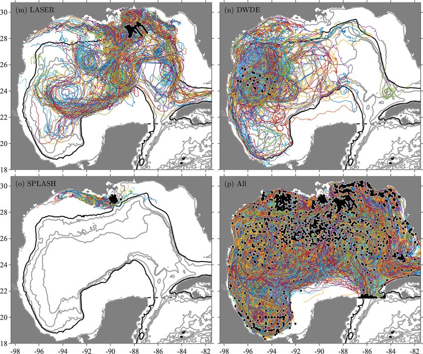
646                                                            J. M. Lilly and P. Pérez-Brunius: Gulf of Mexico surface currents

currents are an invaluable resource with unprecedented spa-             The societal importance motivating studies of the Gulf
tial and temporal continuity, their spatial resolution cannot        of Mexico has a flip side that one must also contend with.
match those derived from dense surface drifter deployments.          Owing to economic interests in the region, some important
Whereas satellite altimetry employs an O(100) km smooth-             datasets are proprietary and are not publicly shared. By far
ing scale, surface drifters can resolve fluctuations as small as     the largest is that belonging to Horizon Marine, part of the
hundreds of meters or even meters depending on the tracking          Woods Hole Group, and described by Anderson and Sharma
method employed.                                                     (2008) and Sharma et al. (2010). This dataset was recently
   These drifter experiments have been previously exploited          used by Mulet et al. (2021) together with several other drifter
for their scientific content on an individual basis. However,        datasets to create an experimental product of daily velocity
they retain great latent value as possible components of an          maps from merged altimetry and drifter measurements. Un-
aggregate. As the various datasets have complementary spa-           fortunately, this product is only available for a brief 8-month
tial and temporal distributions, there is much to be gained          time period, from 1 August 2015 to 30 April 2016. As a part
by combining them. Other authors, e.g., Miron et al. (2017),         of a research project in the Gulf of Mexico, we have obtained
Gough et al. (2019), and Mulet et al. (2021), have compiled          access to a subset of the Horizon Marine data, as well as
merged datasets similar to the one created here and success-         to a second proprietary dataset, the Southern Gulf of Mex-
fully employed these for their own purposes. Yet there cur-          ico (SGOM) dataset owned by the state-owned Mexican oil
rently exists no publicly distributed merged data product de-        company Petróleos Mexicanos (Pemex).
rived from Gulf of Mexico surface drifters. Indeed, the only            In order that other researchers may benefit from the valu-
mean circulation maps for the Gulf of Mexico from drifter-           able set of historical drifter measurements in the Gulf of
derived datasets that we have identified in the literature since     Mexico, a spatially and temporally gridded velocity product
DiMarco et al. (2005) and Nowlin et al. (2001), at a time            is created. This product includes data from the proprietary
when the data coverage was a fraction of what it is today,           datasets that are available to us, working around the nonnego-
are those appearing within global maps that are based exclu-         tiable constraint that the trajectories themselves are not dis-
sively on drifters from NOAA’s Global Drifter Program (e.g.,         tributable. This data product, called GulfFlow, is intended to
Lumpkin and Johnson, 2013; Laurindo et al., 2017).                   facilitate studies of the mean circulation and its interannual
   Accessing the information content of the historical drifter       and seasonal variability. It contains all velocities from all data
observations in the Gulf of Mexico is challenging for a num-         sources bin-averaged into either 1/4 or 1/12◦ spatial bins
ber of reasons. To begin with, many of these experiments             and into overlapping 1-month-long temporal bins spaced ev-
were carried out before the practices of data sharing and data       ery half month from July 1992 until July 2020. The number
archiving had evolved into their current efficient and rigorous      of velocity data points from each of the source datasets con-
form. Consequently, the investigator wishing to make use of          tributing to each bin in the 3D spatiotemporal grid is also
datasets that appear in the literature has to first track down       recorded. GulfFlow is freely distributed for noncommercial
these data by navigating government or institutional archiv-         use, as described in Sect. 6.
ing sites with varying degrees of user friendliness, as well as         The gridded datasets have the advantage that high-quality
obscure individual project sites, or in some cases by person-        mean flow estimates are readily obtained through averaging
ally contacting the investigators. The data products one then        over their time dimension. By contrast, averaging drifter data
collects are generally presented in a range of custom ascii          from all times into spatial bins leads to a distorted mean flow
formats that one must write custom code to read.                     map. This is a result of the highly inhomogeneous temporal
   After this, one is faced with the task of combining a het-        sampling that tends to bias the maps in a direct average. The
erogeneous group of datasets having different sample rates,          improvement in performance due to the two-step temporal
states of processing, and physical drifter designs and having        averaging can be quantified by applying the same averaging
been subjected to a variety of upstream quality control, in-         methods to altimetrically inferred velocities and to velocities
terpolation, and filtering procedures. Some datasets are dis-        from numerical models of the region, sampled along the lo-
tributed with extensive metadata including error estimates           cations of the observed drifter trajectories.
from the interpolation, while others include only interpolated          In addition to these two gridded datasets, a merged hourly
latitude and longitude values with no indication of how these        dataset, called GulfDrifters, is created. This contains quality-
relate to the original position fixes. Some are on regular tem-      controlled and uniformly processed versions of all available
poral grids with no gaps, some are on regular grids with occa-       surface drifter data from the Gulf of Mexico. Drifter loca-
sional gaps, and one dataset is presented in its raw, ungridded      tions, velocities derived from these, a bad or missing data
form. Thus the challenge to the analyst is to combine this in-       flag created during this processing, and drogue flag metadata
formation in a sensible way. One wishes to keep the metadata         from the original sources when available are all incorporated
in the situations when it is available, and when it is not avail-    as a part of this product. It is created in two different versions,
able one would like to use subjective and objective means to         GulfDriftersAll – the basis for GulfFlow – and GulfDrifter-
identify suspicious or problematic intervals.                        sOpen; the latter has three proprietary datasets removed and
                                                                     is distributed without restriction, as described in Sect. 6.

Earth Syst. Sci. Data, 13, 645–669, 2021                                               https://doi.org/10.5194/essd-13-645-2021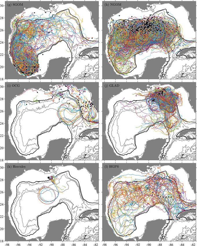
J. M. Lilly and P. Pérez-Brunius: Gulf of Mexico surface currents 647
with the creation of the mean flow map are addressed. Con-
clusions are given in Sect. 7, and data availability is discussed
in Sect. 6. Finally, Appendix A gives some details of the nu-
merical processing with reference to a freely available soft-
ware package for data analysis maintained by the first author.
2 An improved surface current map
The best currently available estimated time-mean surface
current maps for the Gulf of Mexico, created from two very
different sources, are shown in Fig. 2 together with two maps
created in this paper. All of these velocity maps are on the
same 1/4◦ grid.
The mean surface currents over the time period 1 January
1993 until 13 May 2019 from a satellite-altimeter-derived
velocity product are shown in Fig. 2a. This product is dis-
tributed by the Copernicus Marine Environment Monitoring
Service (CMEMS) and is essentially the same product that
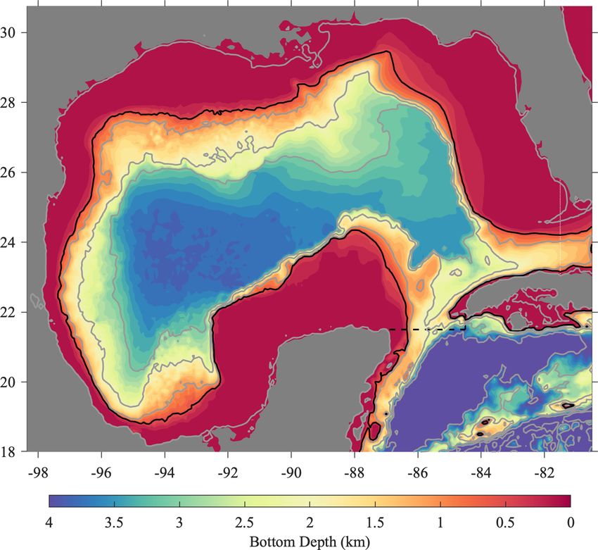
Figure 1. Bottom depth in the Gulf of Mexico, in kilometers. The was previously distributed by the Archiving, Validation and
region within which drifter trajectories are extracted is bounded by Interpretation of Satellite Oceanographic Data (AVISO) ser-
80.5◦ W to the east, the right-hand edge of this plot, and in the Yu- vice. It involves a substantial amount of spatial smoothing –
catán channel by the dotted line extending east from the Yucatán the result of an optimal interpolation – with zonal smoothing
Peninsula along 21.5◦ N and turning north to Cuba at 84.5◦ W. The scales of around 170 km at the latitude of the Gulf of Mexico
heavy black contour is the 500 m isobath, while the gray contours (see Fig. 4a of Pujol et al., 2016). As it is based on differenti-
mark the 5 m isobath as well as those at 1, 2, etc., km. Subsequent
ating a sea surface height anomaly measurement, this product
plots will extend eastward only to 81.5◦ W, the dashed white line
reaching from Florida to Cuba.
represents only the geostrophic part of the surface currents.
The Gulf of Mexico portion of the global time-mean sur-
face currents from the climatology produced by Laurindo
et al. (2017) is shown in Fig. 2b. This product, created by
For reference, the bathymetry of the Gulf of Mexico is NOAA’s Atlantic Oceanographic and Meteorological Labo-
shown in Fig. 1, together with a delineation of the study re- ratory (AOML) using data from AOML’s Global Drifter Pro-
gion. The Gulf of Mexico is characterized by a broad shelf gram (GDP) drifters, will be referred to as the Near-Surface
with depths of 500 m or less, nearly encircling a deep basin Velocity Climatology or NSVC. Drifter velocities, corrected
with depths as great as 3.5–4 km. The shelf system consists for slip bias in the case of drogue loss, are subjected to a spa-
of the Yucatán Shelf (also known as the Campeche Bank) to tiotemporal fit for all GDP data points within a radius equiv-
the south, the Texas–Louisiana Shelf to the north, the West alent to 1◦ of longitude, or about 100 km at these latitudes.
Florida Shelf to the east, and the narrower East Mexico Shelf Thus, like the altimetry product, this map involves a spatial
to the west. On the eastern side, relatively shallow sills at smoothing.
the Yucatán Channel and the Florida Straits provide narrow In both maps, the Loop Current is plainly visible and ap-
openings for the entrance and exit of the poleward-flowing pears similar in size, shape, and magnitude. A cyclonic gyre,
Loop Current. These two straits provide natural cutoffs for known as the Campeche Gyre (Padilla-Pilotze, 1990; Pérez-
the study region. Here we define the Gulf of Mexico to be Brunius et al., 2013), is seen in the southwestern Gulf of
bounded to the east by the line 80.5◦ W and to the south by Mexico in Fig. 2b but is only very faintly present in Fig. 2a.
the line extending eastwards from the Yucatán at 21.5◦ N, A southward current near the 500 m isobath off the coast
then turning north toward Cuba at 84.5◦ W. of Florida is seen in both products, although it is stronger
The structure of the paper is as follows. The most funda- in the drifter-derived product. A northward current occurs
mental result from this study, an improved surface current near the western edge of the Gulf of Mexico in the drifter
map, is presented in Sect. 2 and compared with the best cur- product that is only barely apparent in the altimeter prod-
rently available products. The various data sources are de- uct. These are the major features of note that can be seen in
scribed in detail in Sect. 3, with the processing steps for the currently available velocity products. The differences be-
creating the merged dataset presented in Sect. 4. Special at- tween the two products are likely primarily due to the larger
tention is given to possible error and bias sources associated smoothing scales in the altimeter product, although the fact
with the merged drifter dataset. The construction of the grid- that altimetry resolves only geostrophic velocities may also
ded dataset is accomplished in Sect. 5, and errors associated play a role.
https://doi.org/10.5194/essd-13-645-2021 Earth Syst. Sci. Data, 13, 645–669, 2021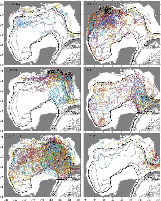
648 J. M. Lilly and P. Pérez-Brunius: Gulf of Mexico surface currents
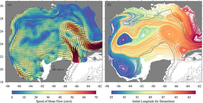
Figure 2. The mean surface circulation in the Gulf of Mexico in 1/4◦ bins from (a) CMEMS satellite altimetry, (b) the global climatology of
Laurindo et al. (2017) using data from NOAA’s Global Drifter Program, (c) a direct bin-averaging of all data in the GulfDriftersAll dataset,
and (d) the time mean of monthly data from the GulfFlow-1/4◦ product, equivalent to a two-step temporal averaging of the GulfDriftersAll
dataset. The colored shading gives the speed of the time-mean flow, also proportional to the length of the arrows. The scale for the arrows is
shown in panel (a). For presentational clarity, arrows are shown on a decimated 3/4◦ grid. Bathymetric contours in this and following plots
are as in Fig. 1.
The lower two panels of Fig. 2 show the estimated mean Directly bin-averaging all good velocity points from the
flows formed from the consolidated drifter dataset created consolidated drifter dataset yields the map shown in Fig. 2c.
here, using two different averaging methods. In both cases, While we see much new detail in the western coastal current
all available drifter data have been utilized, regardless of and the Campeche Gyre, this map is obviously unsatisfac-
drogue depth and whether the drogue was estimated to be tory in the region of the Loop Current. It is shown in Sect. 5
present, absent, or of unknown status. Bins that draw from that its distorted appearance arises as a consequence of the
six or fewer hourly measurements have been omitted in or- extremely inhomogeneous distribution of the data over time.
der to avoid artifacts from insufficient sampling. This naïve method of averaging overemphasizes the state of
the Gulf of Mexico currents during densely sampled time pe-
Earth Syst. Sci. Data, 13, 645–669, 2021 https://doi.org/10.5194/essd-13-645-2021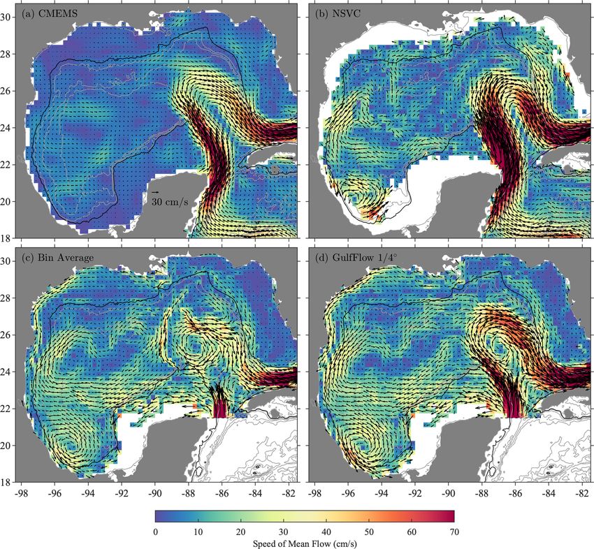
J. M. Lilly and P. Pérez-Brunius: Gulf of Mexico surface currents                                                              649

riods of several large experiments, severely biasing the re-        particular, the Mississippi outflow region in Fig. 3a clarifies
sults toward different time periods in different regions.           the jumble of vectors seen there in Fig. 2d. What is happening
   This problem is addressed by a two-step averaging pro-           in the 1/4◦ map is that the grid is not fine enough to resolve
cedure. For this we use the GulfFlow-1/4◦ product created           the plume structure, leading to vectors in adjacent bins that
here, which has all drifter data averaged in 1/4◦ bins and          seem unrelated to one another. When the grid is fine enough
overlapping monthly bins spaced every half month for 28             to resolve the structure, the same data lead to the meaning-
years. Averaging over the temporal bins leads to the map            ful outflow pattern seen in Fig. 3a. High-resolution modeling
shown in Fig. 2d. The sampling artifacts affecting the direct       studies such as that of Barkan et al. (2017) also show strong,
bin average in Fig. 2c have been satisfactorily removed. The        narrow outflow plumes in this region; see their Fig. 8.
apparently superior performance of this averaging method,              The streamlines corresponding to the 1/12◦ mean flow
while impossible to assess directly from observations, can          map, in Fig. 3b, emphasize the closed circulations in the
be estimated by applying the same sampling and averaging            Campeche Gyre and in the central and western deep Gulf of
schemes to the CMEMS altimeter fields as well as to the out-        Mexico. Closed time-mean circulations within the center of
put of several high-resolution numerical models. This is done       the Loop Current, and within a triangular region between the
in Sect. 5, in which we find the estimated reductions in error      base of the Loop Current and Cuba, are also seen. As pointed
to be in the range of 32 %–44 %.                                    out by an anonymous reviewer, the small closed cyclonic cir-
   Note that the average over overlapping time bins is virtu-       culation to the north of the Loop Current most likely reflects
ally identical to averaging over only all whole-month bins.         the impact of the intense cyclonic eddies formed in the shear
The semimonthly temporal spacing in GulfFlow is chosen              zone on the periphery of the Loop Current – the Loop Cur-
such that seasonal variability can be better resolved, so we        rent Frontal Eddies (LCFEs) – that are found frequently in
simply average over all temporal bins for convenience.              this area; see Le Hénaff et al. (2014) and references therein.
   Unlike the first row of Fig. 2, the second row involves          This figure also reveals a robust east–west connectivity over
no spatial averaging apart from the 1/4◦ bin-averaging.             the deep part of the Gulf of Mexico, with streamlines reach-
Consequently, features are seen at much higher resolution.          ing over some 10◦ of longitude, presumably largely reflecting
A southward-flowing coastal current is revealed, extending          the average flow associated with the westward-propagating
from Louisiana to about 24◦ N, that is entirely absent from         Loop Current Eddies. Strong north–south connectivity along
Fig. 2a, b. The northward-flowing shelf-break current near          the western boundary is also seen.
24◦ N in Fig. 2b takes on a more eddy-like or gyre-like shape          The maps in Fig. 3 represent the highest-resolution esti-
in Fig. 2d. At its northern edge, a bifurcation is seen where       mate of the mean Gulf of Mexico surface currents created to
part of the mean current turns to the north while part of it        date. Further examination of the patterns seen here, as well
turns to the east. A large-scale, bean-shaped anticyclonic cir-     as of temporal variability captured by the GulfFlow prod-
culation, with a pronounced velocity minimum along its cen-         ucts, is outside the scope of this paper on the dataset genera-
ter, is seen extending throughout the deep Gulf of Mexico           tion itself. However, this brief comparison illustrates that the
from west of the Loop Current to the western coast. In short,       GulfFlow products are largely in agreement with, but are a
a number of apparently physically meaningful features are           substantial improvement on, other data products for the re-
seen that cannot be discerned in currently available products.      gion.
   This velocity map can be improved still further. A higher-
resolution version of the GulfFlow product, GulfFlow-1/12◦ ,        3     Data sources
is created with 1/12◦ spatial binning instead of 1/4◦ . The
gridded data are averaged over all time slices, weighted by         This section presents in detail the properties of the various
the total number of data points in each bin, and smoothed us-       drifter datasets from the Gulf of Mexico that are aggregated
ing a local parabolic weighting function, 1 − r 2 /R 2 , that de-   here. Drifter data in the Gulf of Mexico are available from
cays to zero at a radius of R = 50 km and that is zero outside      15 different sources, presented in Fig. 4 and listed in Table 1.
of that radius. Mapped values that draw from four or fewer          The figures and table represent the state of the datasets after
nonempty 1/12◦ spatial bins are omitted. The resulting mean         the uniform processing methodology discussed subsequently
flow estimate is shown in Fig. 3a, which again uses observa-        in Sect. 4. Instructions for obtaining the various datasets may
tions for all drogue depths and statuses. A subsequent assess-      be found in Sect. 6, “Code and data availability”, near the end
ment suggests this map, and the corresponding mean stream-          of the paper. The data sources are now described in chrono-
line plot in Fig. 3b, is likely not significantly influenced by     logical order.
bias due to drifter sampling patterns or drogue loss.
   Comparing the smoothed 1/12◦ map in Fig. 3a with the
                                                                    3.1    The Texas-Louisiana Shelf Circulation and
1/4◦ binned map in Fig. 2d, we see that the former has more
                                                                           Transport Study (LATEX)
detail in regions of fine-scale structure such as the counter-
flowing currents of the western boundary current, the Missis-       The Texas-Louisiana Shelf Circulation and Transport Study
sippi outflow plume, and the interior of the Loop Current. In       (LATEX) was an early Lagrangian experiment to study the

https://doi.org/10.5194/essd-13-645-2021                                              Earth Syst. Sci. Data, 13, 645–669, 2021
650                                                                                   J. M. Lilly and P. Pérez-Brunius: Gulf of Mexico surface currents

Figure 3. Panel (a) is the surface circulation in the Gulf of Mexico as in Fig. 2, but for the GulfFlow-1/12◦ product smoothed within 50 km
radius circles as described in the text. Panel (b) shows streamlines of the mean flow in (a), colored according to their initial longitude.

Table 1. Meta-information for the various surface drifter datasets in the Gulf of Mexico after the quality control applied here. From left
to right, the columns are experiment name; drifter type; nominal drogue depth; tracking system; nominal original sample interval 1, in
hours unless otherwise noted; number of different trajectory segments; number of hourly data points after interpolation; percent of these that
qualify as “filled” as described in the text; date of first hourly data point format; date of last hourly data point; mean duration of trajectories
after processing, in days, plus or minus the standard deviation of trajectory durations; and maximum trajectory duration in days. Different
experiments are sorted in order of the date of the first data point appearing in the processed dataset. For the nominal drogue depth, the
approximate extension of the drogue below the water surface is used for the CODE and CARTHE drifters, the mid-depth of the holey sock
drogue is used for the SVP and WOCE drifters, and the nominal parachute depth is used for the FHD drifters. The DWDE contains three
different types of drifters, CODE, Microstar, and DORIS drifters, described further in the text. The last two lines refer to the GulfDriftersAll
dataset – the basis for the GulfFlow gridded product created herein – and the GulfDriftersOpen version containing only publicly available
data.

                                                                       Surface drifter data from the Gulf of Mexico
       Name            Type            Drogue      Tracking            1      Traj.         Points   % Fill      First date      Last date    Duration   Max
       LATEX           WOCE             7.5∗ m     Argos              6.0       19          33 931   2.543     3 Aug 1992      19 Feb 1995     74 ± 73   251
       SCULP1          CODE                1m      Argos              1.5      378         570 159   0.248      2 Jun 1993     29 Jan 1995     63 ± 39   131
       SCULP2          CODE                1m      Argos              1.5      247         387 638   0.839      6 Feb 1996     31 Oct 1996     65 ± 41   224
       GDP             SVP                15 m     Argos              6.0       71         108 161   1.353    25 Sep 1996      21 Apr 2020     63 ± 92   530
       HARGOS          SVP                15 m     Argos              1.0      193         363 336   1.888     20 Jan 1999     22 Apr 2017     78 ± 94   593
       AOML            CODE                1m      Argos           Irreg.       76          76 314   1.934    10 Dec 2003     30 May 2012      42 ± 25    95
       SGOM            FHD                45 m     GPS                1.0      462         511 418       0    25 Sep 2007      21 Sep 2014     46 ± 47   254
       NGOM            FHD                45 m     GPS                1.0      370         461 419   5.108    15 Feb 2010       2 Sep 2014     52 ± 48   273
       OCG             CODE                1m      Argos          0.5/1.0       59          51 208   0.478    30 Apr 2010      29 Jan 2013     36 ± 24    99
       GLAD            CODE                1m      GPS               0.25      297         400 388       0     20 Jul 2012     22 Oct 2012     56 ± 28    94
       Hercules        Tube                1m      GPS             5 min        12           7123    1.347     27 Jul 2013      9 Sep 2013     25 ± 10    43
       HGPS            SVP                15 m     GPS                1.0       44         132 644   0.157     7 Aug 2013     31 Mar 2020    126 ± 136   676
       LASER           CARTHE              1m      GPS               0.25      996         891 174   0.106     20 Jan 2016     30 Apr 2016     37 ± 18    89
       DWDE            Various             1m      GPS                1.5      207         410 972   0.519    21 Jun 2016      18 Apr 2018     83 ± 58   294
       SPLASH          CARTHE              1m      GPS             5 min       339         101 487   5.628    19 Apr 2017       8 Jun 2017     12 ± 11    48
       GD_All          Various         Various     Various            1.0     3770     4507372       1.070    3 Aug 1992      21 Apr 2020      50 ± 49   676
       GD_Open         Various         Various     Various            1.0     2731     3123563       0.721    3 Aug 1992      21 Apr 2020      48 ± 47   676
∗ The LATEX drifters had a 7.5 m drogue depth, apart from three drifters; see Sect. 3.1.

Earth Syst. Sci. Data, 13, 645–669, 2021                                                                          https://doi.org/10.5194/essd-13-645-2021
J. M. Lilly and P. Pérez-Brunius: Gulf of Mexico surface currents                                       651

Figure 4.

https://doi.org/10.5194/essd-13-645-2021                            Earth Syst. Sci. Data, 13, 645–669, 2021
652                                        J. M. Lilly and P. Pérez-Brunius: Gulf of Mexico surface currents

Figure 4.

Earth Syst. Sci. Data, 13, 645–669, 2021                         https://doi.org/10.5194/essd-13-645-2021
J. M. Lilly and P. Pérez-Brunius: Gulf of Mexico surface currents                                                                    653

Figure 4. Surface drifter data in the Gulf of Mexico from 15 different sources, as labeled, together with the combined dataset in the last
panel. Colored lines are different trajectories from the processed dataset, the beginning of each of which is marked by a black dot.

circulation on the Texas–Louisiana Shelf. LATEX-A con-                       drogue bottom at 50 m depth and one (07839) had
sisted of 19 drifters released between August 1992 and                       an even longer tether which placed the drogue bot-
November 1994; see Fig. 4a. Data from a related experiment,                  tom at 100 m depth.
LATEX-C, could not be located. The drifters, referred to as
“WOCE-type” drifters by Howard and DiMarco (1998), are                    Thus the nominal drogue depth of most drifters was at
described by those authors as follows.                                 7.5 m. For these data, raw position estimates from Argos
                                                                       tracking had been spline-fitted onto 6-hourly trajectories. In
     The drifters consisted of a spherical, 33.7 cm di-                our processing, brief initial deployments and recoveries of
     ameter, foam-filled fiberglass surface float attached             drifters 69341 and 78331, lasting only a few days, are omit-
     by a tether to a 91 cm diameter hoop which sup-                   ted.
     ported a 6 m cylindrical drogue made of heavy can-
     vas. The canvas cylinder had a series of circular
                                                                       3.2   The Surface Current and Lagrangian Drift Program
     holes in it, which is why this type of drogue is
                                                                             (SCULP)
     commonly referred to as a “holey-sock”. Eighteen
     drifters had a 3 m tether which placed the bottom of              The Surface Current and Lagrangian Drift Program (SCULP)
     the 6 m drogue, at 9 m depth. Two drifters (07834                 described by Ohlmann and Niiler (2005) consisted of three
     and 07833) had longer tethers which placed the                    separate experiments: SCULP-I, which focused on the

https://doi.org/10.5194/essd-13-645-2021                                                  Earth Syst. Sci. Data, 13, 645–669, 2021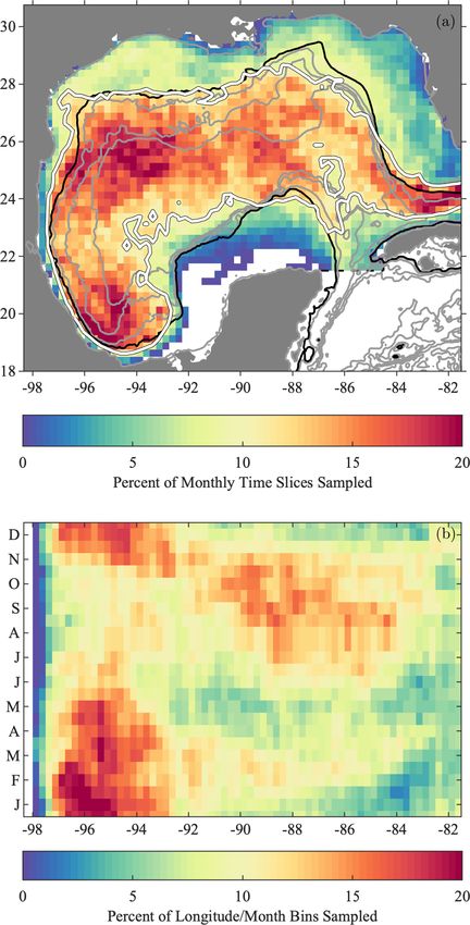
654                                                         J. M. Lilly and P. Pérez-Brunius: Gulf of Mexico surface currents

Texas–Louisiana Shelf beginning in June 1993; SCULP-II,           of the drogues is provided as a part of the GDP dataset as
which focused on the West Florida Shelf beginning in Febru-       described by Lumpkin et al. (2013).
ary 1996; and SCULP-III, which sampled eddies in the Gulf            The standard GDP dataset is a 6-hourly product that uses
of Mexico beginning in April 1998. Of these, only the first       the quality control process of Hansen and Poulain (1996), as
two are available, denoted SCULP1 and SCULP2 here. The            well as the kriging method of interpolation described therein.
trajectories are shown in Fig. 4b, c and are seen to provide      This processing involves heavy interpolation, dating back to
dense coverage over much of the US continental shelf in the       a time when the typical temporal density of position fixes
Gulf of Mexico.                                                   was much less than it is currently. Position fixes were his-
   These experiments used Argos-tracked drifters pat-             torically determined using Argos tracking, but since 2013 a
terned after the Coastal Dynamics Experiment (CODE)               steadily increasing fraction of drifters has been tracked with
drifters of Davis (1985) and manufactured by Techno-              the Global Positioning System (GPS). Further details on this
cean, now MetOcean (https://www.metocean.com/product/             dataset may be found in Lumpkin and Pazos (2007).
codedavis-drifter/, last access: 17 February 2021). These            An updated, higher-temporal-resolution version of this
drifters have submerged sails roughly 1 m wide by 1 m deep        dataset is the hourly product of Elipot et al. (2016, https://
acting as a simple drogue and take the form of a plus sign        www.aoml.noaa.gov/phod/gdp/hourly_data.php, last access:
(+) when viewed from above.                                       17 February 2021), constructed using local polynomial fit-
   Upstream processing of the SCULP datasets is described         ting or “loess” (Fan and Gijbels, 1996; Cleveland, 1979).
by Ohlmann and Niiler (2005) and included despiking by            While the hourly dataset mostly contains data after 2005 –
flagging time points where velocities exceeded 250 cm s−1 .       when a change to the tracking arrangement with Argos led to
A final interpolation step is described therein as follows.       many more position fixes – it also contains some trajectories
                                                                  at earlier times when the average sampling rate happened to
      The despiked position data were then interpolated           be sufficiently high. Drifters tracked by the Argos system and
      onto a uniform three-hour time grid by fitting an           those using the much higher-accuracy GPS tracking are both
      analytic correlation function to the Fourier trans-         included; see Elipot et al. (2016) for a detailed discussion of
      form of a model spectrum based on 10 d of un-               the errors expected for each of these two tracking methods.
      equally spaced data centered on the day of interest            Because of the very different tracking and interpolation
      (Ohlmann et al., 2001; Van Meurs, 1995). The cor-           methods employed, the GDP drifter dataset is separated into
      relation function includes parameters to represent          three distinct portions: hourly Argos (HARGOS) and hourly
      a low-frequency spectral amplitude, a tidal ampli-          GPS (HGPS) trajectories from Elipot et al. (2016), and tra-
      tude, and a tidal peak width.                               jectories from the standard product (GDP). Trajectories that
                                                                  are also in either HARGOS or HGPS are omitted from the
   This represents a very different and more complex interpo-     GDP portion to prevent redundancy. Plots of these trajecto-
lation step than has been employed in any of the other drifter    ries are shown in panels (d), (e), and (l) of Fig. 4. As these
datasets and calls for specialized processing steps to detect     drifters are generally launched outside of the Gulf of Mexico,
occasional oscillatory artifacts, as discussed later. While it    one sees them often entering via the Yucatán Channel. For
appears that such events are rare, and although we have done      the HARGOS dataset one also sees many starting points in
our best to identify suspect time periods, the possibility of     the interior of the Gulf of Mexico, due either to local deploy-
such artifacts should be kept in mind.                            ments or because these mark the starting points of trajectory
                                                                  segments with sufficiently dense sampling to be included in
3.3   NOAA’s Global Drifter Program (GDP) drifters                the hourly product. A tendency to typically not cross from
                                                                  deep water to the shallow waters of the continental shelf is
The United States’ National Oceanic and Atmospheric Ad-           apparent.
ministration (NOAA) produces a large global dataset of
surface drifters through its Global Drifter Program (GDP)         3.4   AOML South Florida Program and hurricane
at https://www.aoml.noaa.gov/phod/gdp/index.php (last ac-               response drifters
cess: 17 February 2021). The physical design of the GDP
drifters is based on instruments developed for the Surface        Drifter trajectories from two small experiments by AOML,
Velocity Program (SVP) of the Tropical Ocean Global Atmo-         the South Florida Program (SFP) and Hurricane Response
sphere (TOGA) experiments; see Lumpkin and Pazos (2007).          Drifters (HRD), both using CODE-type drifters tracked by
Consequently, the drifters employed by the GDP are known          Argos, are shown in Fig. 4f. These drifters do not appear
as “SVP drifters”. While there are several design variants,       to have been used in a previous scientific publication. These
a common feature is a holey-sock drogue centered at 15 m          will be grouped together under the category “AOML”. Most
depth that is intended to reduce wind slippage. Drogues can       of these were deployed at irregular intervals between 2003
be lost during the drifter lifetime, which will alter the re-     and 2012 off the west coast of Florida, although some were
sponse to wind forcing. A flag for the presence or absence        deployed during 2005 on the Texas–Louisiana Shelf. Unlike

Earth Syst. Sci. Data, 13, 645–669, 2021                                           https://doi.org/10.5194/essd-13-645-2021
J. M. Lilly and P. Pérez-Brunius: Gulf of Mexico surface currents 655
all the other datasets used here, these data are distributed in Liu and Weisberg (2011) and Liu et al. (2013b). These
in the form of raw position fixes and therefore require an and the RedTide drifters are CODE-type drifters manufac-
additional processing step. The raw position fixes are bin- tured by Technocean (Yonggang Liu, personal communica-
averaged onto a uniform hourly grid, then gaps up to 6 h are tion, 17 August 2015) and tracked by Argos (Jeff Dono-
filled with interpolation using a piecewise cubic Hermite in- van, personal communication, 18 August 2005). The tem-
terpolation polynomial, also known as the “pchip” method. poral resolution was hourly with occasional gaps for most of
the drifters, with a subset of 36 OilSpill drifters having half-
3.5 Southern and Northern Gulf of Mexico experiments
hourly resolution.
(SGOM and NGOM)
3.7 The Grand Lagrangian Deployment (GLAD)
Two datasets analyzed in this project use Far Horizon
Drifters (FHD) manufactured by Horizon Marine, now a part The Grand Lagrangian Deployment (GLAD; Özgökmen,
of the Woods Hole Group (http://woodsholegroup.com, last 2013; Poje et al., 2014) was a major experiment designed to
access: 17 February 2021), consisting of a cylindrical sur- examine dispersion in the aftermath of the Deepwater Hori-
face buoy attached to a 45 m line terminating in a 1.2 m zon oil spill. This experiment was carried out by the Consor-
parachute-style drogue. These instruments are deployed by tium for Advanced Research on Transport of Hydrocarbon
air, during which process the drogue doubles as an actual in the Environment (CARTHE). The GLAD experiment uti-
parachute, and record their positions at hourly intervals us- lized ≈ 300 CODE-type drifters with GPS tracking. Trajec-
ing GPS. The Far Horizon Drifters are discussed in Ander- tories are shown in Fig. 4j. Distinguishing features of this ex-
son and Sharma (2008) and Sharma et al. (2010). Unlike the periment are that the drifters were launched within 3 weeks
SVP-type drifters, there is no automated mechanism for de- of each other and were grouped into triplets, separated by
tecting drogue presence, nor a study of drogue presence as about 100 m, in order to study small-scale dispersion.
far as we are aware; thus one should be aware of the poten- Detailed information as to the data processing is dis-
tial impact of wind slippage, discussed further subsequently. tributed with the data. Position fixes were obtained roughly
The first dataset of this type is the Southern Gulf of Mex- every 5 min. Data points were then flagged as bad if veloci-
ico (SGOM) drifters; see Fig. 4g. An earlier version of this ties exceeded 300 cm s−1 or met several other quality-check
dataset was previously utilized in a study by Pérez-Brunius criteria. Valid positions were then spline-interpolated to uni-
et al. (2013). According to those authors, three to five drifters form 5 min time intervals, filtered with a 1 h low-pass filter,
were air-deployed every month in the Bay of Campeche and finally interpolated onto a 15 min temporal grid. Drifter
south of 20.5◦ N beginning in October 2007; this deployment records end when the drifter was determined to have been
continued through mid-2014. A second set of Far Horizon picked up by a boat, when the signal was lost for more than
Drifters is the Northern Gulf of Mexico (NGOM) dataset 24 h, or when the drifter displacement exceeded 80 km in a
seen in Fig. 4h, largely contemporaneous with the SGOM 12 h period.
dataset but deployed in the US waters. An important point is Since the interest in this experiment was on short-
that the NGOM drifters were preferentially deployed in order timescale dispersion, the drifters were not tracked for a par-
to sample eddies as a part of Horizon Marine’s EddyWatch ticularly long period of time. Drifter records end abruptly on
program and therefore do not represent an independent and 22 October 2012 with no trajectories longer than 95 d; see
unbiased sampling of the circulation. Table 1 and also the subsequent Fig. 5. Therefore, this exper-
In the upstream processing of both of these datasets, posi- iment represents an intensive sampling over a short time.
tion fixes were linearly interpolated between gaps, and data
points were then flagged as bad if position fixes were located 3.8 The Hercules experiment
on land, if speeds exceeded 300 cm s−1 , and during gaps of
larger than 6 h. Hercules was a relatively small experiment with 19 drifters
launched near the site of the Hercules 265 drilling rig in
3.6 Ocean Circulation Group (OCG) drifters
July 2013 and intended to track dispersion in the aftermath
of an explosion on that rig (Özgökmen, 2014; Weber et al.,
A relatively small set of drifters is available from the Ocean 2016), shown in Fig. 4k. The drifters were tracked with GPS
Circulation Group (OCG) at the University of South Florida. with positions reported every 5 min. The drifter designs were
These data are from two separate experiments, the OilSpill of two different experimental types, 13 of type A and 6 of
experiment in the immediate aftermath of the Deepwater type B. However, visual inspection shows that the trajectories
Horizon oil spill in April 2010, with deployments on the from type B drifters are apparently poorly sampled and also
West Florida Shelf, and a very small coastal experiment of short duration, and consequently these six are discarded.
in 2012 called RedTide deployed on the Texas–Louisiana The type A drifters are described in the dataset documenta-
Shelf. Drifters from both experiments are grouped together tion as having a “plastic, tubular body roughly 50 cm high”
and shown in Fig. 4i. The OilSpill drifters were analyzed and will be denoted “tube”-type drifters. These may be con-
https://doi.org/10.5194/essd-13-645-2021 Earth Syst. Sci. Data, 13, 645–669, 2021656 J. M. Lilly and P. Pérez-Brunius: Gulf of Mexico surface currents
sidered related to the CODE drifters in that they are drogued above. During both years, a small number of drifters were
close to the surface. of the “DORIS” type, a simple drifter manufactured by the
Observatorio Oceanográfico Regional Costero group from
3.9 The Lagrangian Submesoscale Experiment
Universidad Nacional Autónoma de Baja California, Méx-
(LASER)
ico (see http://www.cienciamx.com/index.php/tecnologia/
tic/14762-doris-sonda-oceanografica-iio-uabc, last access:
The goal of the recent Lagrangian Submesoscale Experiment 17 February 2021). Of the 207 total drifters, 98 were of the
(LASER), also carried out by CARTHE, was to examine dis- Microstar type, 88 were of the CODE type, and 21 were of
persion by submesoscale processes in wintertime conditions the DORIS type. Upstream processing was the same as for
in the northeastern Gulf of Mexico (D’Asaro et al., 2017; the SGOM experiment.
Haza et al., 2018). For this experiment, an innovative new
type of drifter – the CARTHE drifter – was designed that
3.11 Submesoscale Processes and Lagrangian
is inexpensive, mostly biodegradable, and easy to deploy in
Analysis on the Shelf (SPLASH)
large numbers (Novelli et al., 2017; Lumpkin et al., 2017). It
consists of a GPS-tracked toroidal float connected to a plus- The Submesoscale Processes and Lagrangian Analysis on
shaped drogue that extends about 60 cm below the surface. the Shelf, or SPLASH, experiment was designed to study
Laboratory experiments (Novelli et al., 2017) showed that nearshore dispersion in the Louisiana Bight in the spring
the drifting characteristics of the CARTHE drifters are es- of 2017 (Huntley et al., 2017). More than 300 GPS-tracked
sentially identical to those of the earlier CODE drifters. CARTHE-type drifters were released. The dataset used here
Over 1000 CARTHE drifters were deployed in January has been pchip-interpreted to 5 min intervals after removing
and February 2016 in the northeastern Gulf of Mexico, in points with velocities exceeding 262 cm s−1 or accelerations
the vicinity of DeSoto Canyon; see Fig. 4m. These were de- above 1.0 cm s−2 . While in general no drogue presence flag is
ployed in three sets of more than 300 drifters each, again available for these drifters, a small number (13 of 339) were
with many of the drifters deployed in triplets in order to study launched as undrogued drifters, and the drogue flag for these
dispersion, and rapidly spread throughout the Gulf of Mex- drifters is consequently set to “missing.” This dataset does
ico. Like GLAD, this experiment represents a very intensive not appear to have yielded scientific publications at the time
sampling over a short time, with no trajectories longer than of this writing.
90 d. It was found during this experiment that the CARTHE
drifters occasionally lose their drogues, so consequently a
drogue presence flag was determined by Haza et al. (2018) 3.12 Other datasets
by analyzing both trajectory response and transmission in- Apart from the previously discussed proprietary Horizon
formation and distributed as Haza et al. (2017). The drifter Marine drifters used in Mulet et al. (2021), which are not
design was later improved to help prevent this problem in the freely available and to which we only have access for that
future (Novelli et al., 2017). portion in the NGOM experiment, the above datasets repre-
sent nearly all remotely tracked surface drifter experiments
3.10 The Deep Water Dispersion Experiment (DWDE) conducted in the Gulf of Mexico that are referred to in the
peer-reviewed literature. Nowlin et al. (2001) mention an-
The Deep Water Dispersion Experiment (DWDE) was de- other small early experiment conducted during the 1990s,
signed to study dispersion in the deep western Gulf of Mex- NEGOM, that we have been unable to locate. This along
ico. This experiment was carried out by CICESE in four sep- with the LATEX C and SCULP-III experiments, mentioned
arate deployments, with a total of 207 drifters: 21–24 June above, appear to have been lost.
2016 (45 drifters), 15–19 October 2016 (55 drifters), 25–
29 April 2017 (56 drifters), and 7–10 November 2017 (51
drifters). This experimental design allowed the surface veloc- 4 GulfDrifters, a consolidated drifter dataset
ity field to be sampled with relatively high spatial resolution
in two different seasons and in two different years. DWDE All datasets described in the previous section are subjected
is available only for noncommercial use (see Sect. 6), and as to a uniform processing methodology. The result is a quality-
such it cannot be included as a part of our freely distributed controlled dataset, called GulfDrifters, that has been interpo-
drifter dataset, though investigators can access it separately. lated onto an hourly time grid, with time points correspond-
DWDE used drifters of three different designs, all tracked ing to gaps filled during our interpolation flagged as such.
by GPS and all with a 1 m drogue depth. In the first The processing steps are described in this section, followed
two deployments, most were Microstar drifters as used in, by a discussion of bias and error sources and finally a pre-
for example, Ohlmann and White (2005), which register sentation of the sampling properties of GulfDrifters itself.
a flag if their drogue is lost. In the second two deploy- GulfDrifters is created in two versions, GulfDriftersAll that
ments, most drifters were of the CODE type described is the basis for GulfFlow and GulfDriftersOpen that contains
Earth Syst. Sci. Data, 13, 645–669, 2021 https://doi.org/10.5194/essd-13-645-2021J. M. Lilly and P. Pérez-Brunius: Gulf of Mexico surface currents 657
only publicly available data (excluding NGOM, SGOM and 0.1 cm s−1 or greater than 250 cm s−1 are flagged, as well as
DWDE) and that is freely distributed as described in Sect. 6. those failing to pass a minimum acceleration criterion. The
minimum acceleration criterion identifies times for which the
4.1 Uniform processing
acceleration magnitude |u0 (t) + iv 0 (t)|, smoothed with a 168-
point (2-week) Hanning filter, is smaller than 10−4 cm s−2 ;
The uniform processing methodology is as follows. We begin time periods exhibiting such a high degree of smoothness
with data that have been interpolated to a uniform sampling generally either reflect that the drifter is grounded or that
interval, possibly with gaps. Trajectory segments lying en- a data gap has been interpolated over in earlier processing.
tirely within the study region shown in Fig. 1 are isolated. Two criteria are also applied to isolate several unrealistically
Depth is found by looking up drifter positions within the fast segments in shallow water seen in the SCULP datasets.
Smith and Sandwell global 1 min bathymetry dataset v. 19.1 Data flagged at this stage are marked by setting the
(Sandwell and Smith, 1997). Data points for which the depth filled field to true so that they can be excluded from fu-
is negative, indicating a location on land, are flagged as bad. ture analysis, and then the flagged values are re-interpolated
A visual inspection is then carried out in order to iden- over using pchip. The fraction of data points that are filled at
tify trajectory segments that appear suspicious. Several dif- this secondary level is very small, about two every 1000 valid
ferent types of features are interpreted as cause to flag a data data points. Finally, velocity and depth are both re-computed
segment: stationary locations, likely indicating a grounded in the same manner as described above. Processing of the
drifter; extended periods of linearly varying positions, likely SCULP data is double-checked by computing the deviation
indicating a linear interpolation over a data gap; isolated, of the speed from its median value within grid boxes over all
patchy data segments of valid data near the end of a record; drifters and noting no readily evident difference between the
unusually noisy or jagged data segments; high-speed seg- SCULP and non-SCULP speed values.
ments terminating near the shore, likely arising from ground- The result of these processing steps is our consolidated
ing due to wind or wave activity; isolated anomalous points; product, GulfDriftersAll, summarized in the second-to-last
and finally conspicuous, rapidly changing oscillations. Fea- line of Table 1 and presented in Fig. 4p. A second version,
tures of this last type are seen only in the SCULP drifters and GulfDriftersOpen, which excludes the NGOM, SGOM, and
apparently indicate a gap that has been filled with the vig- DWDE datasets for reasons discussed earlier, is summarized
orous interpolation applied to those datasets. Such features in the last line of Table 1 and is distributed to the community
are clearly distinguished from eddies in that they appear as without restriction as discussed in Sect. 6. Note that DWDE
“knots” rather than loops when viewed on a map. is separately available for noncommercial use.
All data points that have been flagged as bad or missing are
removed. The data are then interpolated to a uniform hourly 4.2 Bias and error considerations
spacing using interpolation with a piecewise cubic Hermite
interpolation polynomial, also known as the pchip method. The GulfDrifters dataset is quite heterogeneous, reflecting
A filled flag is created to indicate when this interpola- different drifter designs, drogue depths, and tracking meth-
tion has been applied. Within the hourly dataset, the filled ods, as well as variation in the upstream interpolation and
value of an interpolated data point is set to true if no valid un- processing steps. These differences, as well as other sources
interpolated data points were present within plus or minus of potential bias or error, will now be discussed in more de-
3 h. In the case of the hourly HARGOS and HGPS datasets, tail. For references the temporal extent of the various compo-
a field is available that gives the time gap that has been in- nent experiments is presented in Fig. 5a, while distributions
terpolated over in the upstream interpolation. For these two of the trajectory durations are shown in Fig. 5b.
datasets, our filled flag is also set to true if the time gap in The most obvious distinction between the experiments is
the upstream interpolation exceeds 6 h. For the other datasets, drifter design. Due to the different drogue depths listed in
similar information regarding upstream interpolation gaps is Table 1, the various experiments track the currents at differ-
not available. ent depths. Moreover, there is the issue of possible drogue
From this interpolated hourly dataset, velocity is com- loss. The CODE-type and tube-type drifters are unlikely to
puted using the first central difference on the sphere; see Ap- transmit in the absence of a drogue due to their construc-
pendix A. Trajectory beginning or ending segments lacking tion. For the others, drogue loss is a concern as it impacts the
good data are discarded, as are any trajectories containing no wind slip. For the SVP-type drifters, the impact of drogue
good data. The remaining trajectories from all experiments loss is to increase the wind slip from 0.1% of the 10 m wind
are combined, with a source field added to indicate the speed to 0.7 %–1.6 %; see Laurindo et al. (2017) and refer-
originating dataset. The drifter design type is also recorded ences therein. For the CARTHE drifters, Novelli et al. (2017)
with a type field. report that drogue loss increases the wind slip from less than
Next, acting on the combined hourly dataset, several ob- 0.5 % of the 10 m wind speed to as much as 2 %. We are un-
jective criteria are applied to identify possibly problematic aware of published results for the Far Horizon Drifters.
points. Data points having instantaneous speeds less than
https://doi.org/10.5194/essd-13-645-2021 Earth Syst. Sci. Data, 13, 645–669, 2021658 J. M. Lilly and P. Pérez-Brunius: Gulf of Mexico surface currents
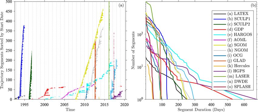
Figure 5. Temporal ranges (a) and duration distributions (b) of drifter trajectory segments from the various sources, after the processing
described in Sect. 4.1, with the color key shown in panel (b). In panel (a), each small horizontal line marks the temporal range of a different
drifter trajectory. The y axis is the trajectory segment number within each data source, sorted in order of the date of the first measurement
point. For display purposes, the upper limit of the y axis is set to 500 trajectories, although the LASER experiment has nearly 1000 trajecto-
ries. In panel (b), the lines show the number of trajectories exceeding a specified duration with a logarithmic y axis. The lower limit of the y
axis is 1 and gives the duration of the longest trajectory segment in each dataset.
Drogue presence flags are available for all of the SVP- altimetry. Both results show that the FHD drifter
type drifters (GDP, HARGOS, and GPS), see Lumpkin et al. data represent well the meso- and large-scale fea-
(2013), as well as for the CARTHE drifters used in the tures of the velocity field in the upper layer of the
LASER experiment (Haza et al., 2018) and the Microstar Bay of Campeche.
drifters used in about half of the DWDE dataset. Since the de-
This indicates that drogue loss from the Far Horizon
sign of the CODE-type drifters (SCULP, AOML, OCG, and
Drifters is unlikely to present a significant problem for cal-
GLAD), and that of the tube-type drifters used in Hercules,
culating gridded statistics.
makes them unlikely to lose their drogues without being de-
The various experiments differ in their temporal distribu-
stroyed, these types of drifters may be regarded as always
tions, another factor that can affect the ways that these ex-
drogued. A drogue presence flag is not currently available for
periments sample the circulation. The temporal distributions
the Far Horizon Drifters (SGOM and NGOM), the CARTHE
are clearly seen in Fig. 5a. Whereas some experiments (e.g.,
drifters used in SPLASH, or the DORIS drifters used in about
GLAD, Hercules, LASER, and SPLASH) involved sudden
10 % of the DWDE dataset.
deployments and also sudden terminations, lasting only a
The biggest potential problem regarding unknown drogue
few months, others (e.g., SGOM, NGOM, and DWDE) in-
status concerns the Far Horizon Drifters, as these make up
volved deployments over a long period of time. The GDP
more than a one-fifth of the drifters in GulfDriftersAll. A
group of drifters – GDP, HARGOS, and HGPS – is different
drogue status flag could be created by examining the re-
from the others in that they generally enter the Gulf of Mex-
sponse of the drifters to wind forcing, following Lumpkin
ico by chance, also leading to temporal distributions that are
et al. (2013) and Haza et al. (2018); however, this substan-
spread out in time. As mentioned above, NGOM is unique in
tial undertaking is outside the scope of this paper. Examin-
that it was from a program to monitor eddies and therefore
ing correlations of different types of drifters with winds and
may contain a bias toward a state of eddy presence.
with currents from CMEMS gridded products in a study of
A less obvious distinction between experiments is the dif-
the Bay of Campeche circulation, Pérez-Brunius et al. (2013)
ference in trajectory durations. As seen in Fig. 5b, durations
concluded that
for the various experiments fall into three groups that appear
the FHD drifter data have the same correlation with to reflect the drifter designs. The longest-duration trajectories
the winds as the 15-m drogued SVP drifters from are all associated with SVP-type drifters in the GDP, HAR-
the Poulain et al. (2002) study, and are highly cor- GOS, and HGPS datasets, each of which have at least one
related with the geostrophic currents derived from trajectory exceeding 400 d. Moreover, these duration curves
Earth Syst. Sci. Data, 13, 645–669, 2021 https://doi.org/10.5194/essd-13-645-2021J. M. Lilly and P. Pérez-Brunius: Gulf of Mexico surface currents 659
have a shallower slope than those for the other experiments, 4.4 A naïve mean flow map
indicating that the SVP drifters are more likely to experi-
ence long lifetimes. Among the shortest-lifetime experiments The most obvious way to form an estimated mean flow from
are GLAD, LASER, and SPLASH, with their sudden cut-off the drifters is simply to take the average of all available ve-
times, none of which have trajectories exceeding 100 d. One locities within each spatial bin. The result, presented earlier
also sees the CARTHE-type drifters (LASER and SPLASH) in Fig. 2c, is seen to have a distorted and unrealistic appear-
have a steeper slope than other experiments, likely indicating ance in the vicinity of the Loop Current. The reason for this
a higher failure rate. These duration differences mean that can be understood at once by looking at the data distribu-
the ability to resolve the low-frequency behavior also differs tion in Fig. 6. The ridge of high southward velocities to the
among the experiments. west of the Loop Current is coincident with the region of ex-
Another important issue is that of position accuracy. tremely dense sampling due to the LASER experiment.
Whereas the Argos tracking system has typical positioning This is a simple yet important message. When drifter data
errors of hundreds of meters (see Tables 1 and 2 of Elipot are distributed highly inhomogeneously in time, one does not
et al. (2016)) GPS positions are accurate to within a few me- wish to simply average it. Such an average tends to bias the
ters. A very detailed treatment of the errors associated with result towards the state of the system at the times of densest
Argos positioning can be found in Sect. 2.3 of Elipot et al. observations. Fortunately, a small modification in the tempo-
(2016), so we refer the reader there for further details. A ral averaging will lead to a substantial improvement.
practical impact of these tracking differences is that GPS-
tracked drifters have almost no bad data points. While both 5 GulfFlow, 3D gridded velocity products
Argos- and GPS-tracked drifters can be productively used
to study the flow on monthly or longer timescales, the GPS Two factors motivate the creation of gridded velocity prod-
drifters can resolve fast-timescale, small-amplitude signals – ucts for the Gulf of Mexico derived from surface drifters. The
such as internal waves or small-scale vortex motions – that first is a desire to study the mean circulation, along with sea-
are well below the noise level of the Argos-tracked drifters. sonal and interannual variability, in a way that avoids the av-
eraging artifacts just discussed. The second is the aspiration
4.3 Sampling properties to make information derived from the consolidated drifter
dataset available to the community, even if some of the tra-
The spatial distribution of hourly, non-filled observations jectories themselves cannot be distributed.
from GulfDriftersAll in 1/4◦ bins is shown in Fig. 6, together This section describes the creation of the gridded products,
with the most commonly occurring sample source within examines their sampling distributions, and uses them to cre-
those bins. A highly inhomogeneous sampling is seen. The ate the improved maps presented in Sect. 2. Errors relative to
various experiments are complementary, with different ex- the unknown true mean, and the improvement over the naïve
periments dominating in different regions. map of the previous section, are quantitatively estimated.
The Gulf of Mexico is bisected north–south by a ridge
of very high sample densities, seen to be associated with
the LASER experiment. High densities are also seen on 5.1 Creation of the gridded product
the Texas–Louisiana Shelf and West Florida Shelf, respec- A gridded product, called GulfFlow, is created by averaging
tively associated with SCULP1 and SCULP2 together with all available data from the GulfDriftersAll dataset within spa-
LASER. Moderately high densities in the western central tial bins and within overlapping month-long temporal bins
and southern Gulf of Mexico are associated with DWDE and having a semimonthly spacing. Two versions are created,
SGOM, respectively. The Mississippi outflow region is most GulfFlow-1/4◦ that uses 1/4◦ spatial bins and GulfFlow-
commonly sampled by the SPLASH experiment. Low data 1/12◦ that uses 1/12◦ spatial bins. The dataset spans monthly
densities are seen in the southeastern Gulf of Mexico, coin- time bins centered on 16 July 1992 through 1 July 2020 for
cident with the southern three-quarters or so of the Loop Cur- a total of 672 overlapping time slices. Odd-numbered slices
rent. There, deployments elsewhere within the Gulf of Mex- correspond to calendar months, while even-numbered slices
ico tend not to reach, and the dominant sampling is there- run from halfway through one month to halfway through the
fore associated with inflowing GDP, HARGOS, and HGPS following month. In addition to the average velocities within
drifters. Very low or zero densities are observed along most each 3D bin, the count of sources contributing to each bin
of the Yucatán shelf. is also distributed, as is the subgrid-scale velocity variance
An implication of this inhomogeneous sampling pattern is discussed in the next section.
that the currents observed by the consolidated drifter dataset The count variable is a four-dimensional array, the fourth
reflect the flow at somewhat different depths, and also over dimension of which has length 45. This variable gives the
different time periods, in the various regions. number of hourly observations from each source dataset con-
tributing to each three-dimensional bin. Values 1–15 are the
count of velocity observations from drifters from each of
https://doi.org/10.5194/essd-13-645-2021 Earth Syst. Sci. Data, 13, 645–669, 2021You can also read