A multi-season investigation of glacier surface roughness lengths through in situ and remote observation - The Cryosphere
←
→
Page content transcription
If your browser does not render page correctly, please read the page content below
The Cryosphere, 13, 1051–1071, 2019
https://doi.org/10.5194/tc-13-1051-2019
© Author(s) 2019. This work is distributed under
the Creative Commons Attribution 4.0 License.

A multi-season investigation of glacier surface roughness lengths
through in situ and remote observation
Noel Fitzpatrick1 , Valentina Radić1 , and Brian Menounos2
1 Departmentof Earth, Ocean, and Atmospheric Sciences, University of British Columbia, Vancouver, V6T 1Z4, Canada
2 Natural
        Resources and Environmental Studies Institute and Geography Program, University of Northern British Columbia,
Prince George, V2N 4Z9, Canada

Correspondence: Noel Fitzpatrick (nfitzpat@eoas.ubc.ca)

Received: 23 October 2018 – Discussion started: 12 November 2018
Revised: 22 February 2019 – Accepted: 13 March 2019 – Published: 2 April 2019

Abstract. The roughness length values for momentum, tem-        tions and seasons and no evidence of a constant ratio with
perature, and water vapour are key inputs to the bulk aero-     momentum roughness length or each other. Of the tested es-
dynamic method for estimating turbulent heat flux. Measure-     timation methods, the Andreas (1987) surface renewal model
ments of site-specific roughness length are rare for glacier    returned scalar roughness lengths closest to those derived
surfaces, and substantial uncertainty remains in the values     from eddy covariance observations. Combining this scalar
and ratios commonly assumed when parameterising turbu-          method with the remote techniques developed here for es-
lence. Over three melt seasons, eddy covariance observations    timating momentum roughness length may facilitate the dis-
were implemented to derive the momentum and scalar rough-       tributed parameterisation of turbulent heat flux over glacier
ness lengths at several locations on two mid-latitude moun-     surfaces without in situ measurements.
tain glaciers. In addition, two techniques were developed in
this study for the remote estimation of momentum roughness
length, utilising lidar-derived digital elevation models with
a 1 × 1 m resolution. Seasonal mean momentum roughness          1   Introduction
length values derived from eddy covariance observations at
each location ranged from 0.7 to 4.5 mm for ice surfaces and    The turbulent fluxes of sensible and latent heat (QH and QL )
0.5 to 2.4 mm for snow surfaces. From one season to the next,   can form a major component of the surface energy balance
mean momentum roughness length values over ice remained         (SEB) of a glacier and substantially influence its rate of sur-
relatively consistent at a given location (0–1 mm difference    face melt (Hock and Holmgren, 1996; Anderson et al., 2010;
between seasonal mean values), while within a season, tem-      Fitzpatrick et al., 2017). With a lack of direct measurement
poral variability in momentum roughness length over melt-       on glaciers, the bulk aerodynamic method is commonly used
ing snow was found to be substantial (> an order of magni-      to parameterise the turbulent fluxes, requiring input of rough-
tude). The two remote techniques were able to differentiate     ness length values for momentum (z0v ), temperature (z0t ),
between ice and snow cover and return momentum roughness        and water vapour (z0q ). Observations of roughness length
lengths that were within 1–2 mm ( an order of magnitude)       are rare on glacier surfaces, however. The majority of SEB
of the in situ eddy covariance values. Changes in wind di-      studies use values and ratios from previous research on sim-
rection affected the magnitude of the momentum roughness        ilar surface types (e.g. Gillet and Cullen, 2011; Giesen et al.,
length due to the anisotropic nature of features on a melting   2014) or treat roughness lengths as model-tuning parameters
glacier surface. Persistence in downslope wind direction on     (e.g. Braun and Hock, 2004; Sicart et al., 2005) rather than
the glacier surfaces, however, reduced the influence of this    obtaining site-specific measurements. This approach intro-
variability. Scalar roughness length values showed consider-    duces uncertainty into turbulent flux estimation, as the trans-
able variation (up to 2.5 orders of magnitude) between loca-    ferability of roughness lengths between locations and sea-
                                                                sons is unknown. Furthermore, parameterisation of the tur-

Published by Copernicus Publications on behalf of the European Geosciences Union.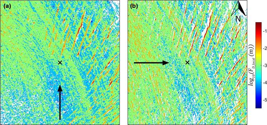
1052                                 N. Fitzpatrick et al.: A multi-season investigation of glacier surface roughness lengths

bulent heat fluxes has been shown in previous studies to be         raphy methods and vertical wind profile measurements to es-
highly sensitive to the implemented roughness lengths (up to        timate z0v at test sites in the Himalayas. Substantial variabil-
a doubling of the calculated flux for 1 order of magnitude          ity in the magnitude of the roughness estimates was noted
increase in z0v ) and to dominate over stability corrections        between the different microtopography methods employed,
as a source of uncertainty (Munro, 1989; Braithwaite, 1995;         with agreement with aerodynamically derived values in some
Brock et al., 2000; Fitzpatrick et al., 2017). The importance       cases.
of accurate roughness length selection, as identified in these         The scalar roughness lengths (z0t and z0q ) are commonly
studies, highlights the need for further research on the spatial    estimated in SEB studies using a fixed ratio with z0v and are
and temporal variability of their values on glacier surfaces        generally assumed to be equal to or 1 to 2 orders of mag-
and on the methods used in their estimation.                        nitude smaller than the momentum roughness length (e.g.
   The roughness length values are defined as the lower lim-        Hock and Holmgren, 2005; Sicart et al., 2005; Hoffman et al.,
its of integration in the bulk gradient or K theory param-          2008). Molecular diffusion controls the rate of scalar trans-
eterisation of the turbulent fluxes (Stull, 1988). z0v can be       fer with a surface and, having a smaller spatial scale than the
thought of as the height above the surface at which wind            form drag processes driving momentum transfer, it is likely
speed, extrapolated downwards along an assumed logarith-            that the scalar roughness lengths would be smaller (Beljaars
mic profile, will reach its surface value. Similarly, z0t and z0q   and Holtslag, 1991). The persistence of this ratio with time is
can be considered to be the heights at which temperature and        uncertain, however. Surface renewal methods have been im-
specific humidity reach their surface values, respectively. z0v     plemented in some studies (e.g. Andreas, 1987; Smeets and
accounts for the effects of form drag on the near-surface wind      van den Broeke, 2008), where variation in this ratio is de-
profile due to the interaction of airflow with features on the      scribed as a function of the roughness Reynolds number R∗ .
surface. In many glacier studies and climate models (e.g. Van       Changes in mean air temperature and relative humidity have
As, 2011; Fausto et al., 2016), z0v values of 1 and 0.1 mm          also been proposed as drivers of scalar roughness length vari-
are used for ice and snow surfaces, respectively, and are of-       ation (e.g. Calanca, 2001; Park et al., 2010).
ten assumed constant with time. Where measurements have                Where EC data are available at the surface of interest,
been obtained on glacier surfaces, however, a large range of        the bulk aerodynamic method is generally implemented to
z0v values have been recorded, with several orders of magni-        calculate in situ roughness length values (e.g. Conway and
tude of variation between different glaciers and seasons (e.g.      Cullen, 2013). Caution is required when applying this tech-
Van den Broeke et al., 2005; Brock et al., 2010). In addition,      nique, however. The bulk method assumes logarithmic pro-
existing values for z0v on glaciers (observed through mast-         files of wind, temperature, and water vapour in the boundary
based vertical wind and temperature profile measurements,           layer, an assumption valid only during neutral atmospheric
or estimated from eddy covariance (EC) observations or mi-          stability conditions (Stull, 1988). During the melt season, the
crotopography surveys) only provided values for an individ-         boundary layer over a glacier is often stable, requiring the
ual location or turbulent footprint. Implementing these single      application of a stability function to the bulk method. These
values in a glacier-wide distributed model or in a point model      stability functions were developed for use over flat terrain,
at another location on the glacier may not account for the po-      however (e.g. Monin and Obukhov, 1954; Dyer, 1974; Bel-
tential variability in surface roughness that may exist across      jaars and Holtslag, 1991), and uncertainty remains regarding
a glacier surface (e.g. Smith et al., 2016).                        their validity over sloped glacier surfaces. Furthermore, pre-
   Efforts have been made in previous boundary-layer studies        vious studies have suggested that some assumptions of the
over different land surfaces to determine momentum rough-           bulk method, namely constant momentum and heat flux val-
ness length values for large areas, including over forestry,        ues with height, may not be valid during katabatic conditions
scrubland, and outwash plains (e.g. Nield et al., 2013; Li          with shallow wind maximums which can develop frequently
et al., 2017). A range of remote-sensing techniques have            in the stable boundary layer over glacier slopes (e.g. Denby
been implemented in such studies, including the use of              and Smeets, 2000). Such conditions may add uncertainty to
light detection and ranging (lidar) systems. Paul-Limoges et        the calculated roughness values due to potential decoupling
al. (2013) used digital elevation models (DEMs), obtained           of turbulence at measurement height from the surface, in-
from airborne lidar, to estimate z0v values over a harvested        termittent and non-stationary turbulence, and the increased
forest surface (z0v = 0.13 m) and found good agreement              importance of advection of turbulent kinetic energy (Denby,
with corresponding EC-derived values (z0v = 0.12 m). Sim-           1999).
ilar studies on mountain glaciers are extremely rare. Smith            The initial goal of this study is to obtain in situ values of
et al. (2016) used terrestrial-based structure-from-motion          the momentum and scalar roughness lengths from multiple
(SfM) photogrammetry and laser surveying to generate a dis-         locations over several seasons. EC-observed data will be im-
tributed map of z0v estimates for a glacier. Meteorological-        plemented into the bulk aerodynamic method to derive these
based evaluation of the returned z0v estimates was not car-         values. The temporal variability of roughness lengths on a
ried out, however. Over debris-covered glaciers, Quincey et         glacier will be examined, and the transferability of values
al. (2017) and Miles et al. (2017) used both SfM microtopog-        between location and years will be assessed. Commonly as-

The Cryosphere, 13, 1051–1071, 2019                                                     www.the-cryosphere.net/13/1051/2019/
N. Fitzpatrick et al.: A multi-season investigation of glacier surface roughness lengths 1053
sumed values and ratios from the literature will be compared passive airflow, while the CPEC analyser has a closed sam-
with the obtained data, and predictive relationships for the ple space into which air is drawn using a pump. Implement-
scalar roughness lengths will be tested. The second goal of ing these methods together helped minimise gaps in the tur-
this study is to develop remote methods for estimating mo- bulence data set (OPEC analysers are susceptible to errors
mentum roughness lengths for a glacier surface, which would during precipitation) and enabled a comparison of their val-
facilitate SEB modelling for glaciers without in situ observa- ues and performance in a glacial environment. The EC data
tions and distributed modelling for glaciers with point mea- were recorded in raw 20 Hz format, with observations from
surements only. Digital elevation models will be obtained for the remaining sensors stored in 1 min averages. Glacier sur-
each study location and will be used to provide surface height face temperature (Ts ) was observed from the infrared surface
data for the two roughness methods developed in the study. temperature sensors in 2015 and 2016 and estimated from the
Turbulence footprint modelling will be employed in one of outgoing longwave radiation observations in 2014 using the
these methods to identify the region of the glacier surface in- Stefan–Boltzmann law (see Fitzpatrick et al., 2017).
fluencing the EC-derived roughness length values. The esti- The meteorological sensors were housed on a four-legged
mates from both remote methods will then be compared with quadpod, which provided a stable platform (verified by an in-
those from corresponding in situ observations. clinometer sensor) that lowered as the ice melted, and main-
tained a constant height of the sensors above the surface. EC
measurements were carried out at a constant height (∼ 2 m
2 Data and methods at each station) to avoid substantially varying the turbulent
footprint area and to reduce the risk of elevating the sensor
2.1 Field campaign
above the turbulence coupled with the surface (Burba, 2013;
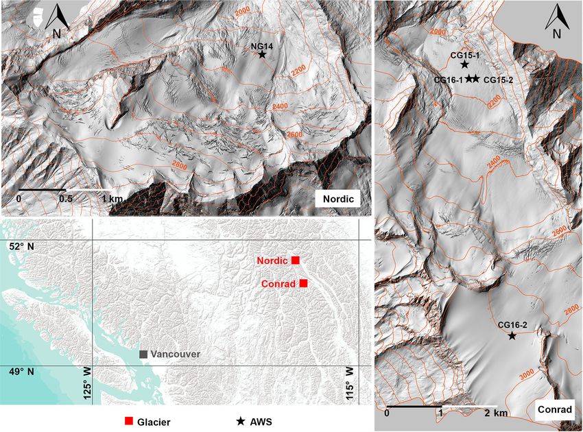
Observations were carried out over three melt seasons (2014– Aubinet, 2008). The turbulent footprint is the source region
2016) on two glaciers in the Selkirk and Purcell Mountains of for the turbulent fluxes received at a given location. It repre-
British Columbia, Canada (Fig. 1). Nordic Glacier (51◦ 260 N, sents the upwind area that influences and contributes to the
117◦ 420 W) is a small (∼ 5 km2 ), north-facing glacier, rang- observed fluxes, and hence, the surface properties that mod-
ing in elevation from 2000 to 2900 m above sea level (a.s.l.), ulate turbulence generation. Broadly speaking, the turbulent
approximately. An automatic weather station (AWS) was in- footprint for fluxes measured at a given height will extend
stalled in the ablation zone of the glacier throughout July and upwind by a distance of roughly 100 times the measurement
August 2014 (NG14). Conrad Glacier (50◦ 490 N, 116◦ 550 W) height (Burba, 2013).
is located 87 km to the southeast of Nordic Glacier, with The installation site for each station was selected based
an area of ∼ 15 km2 and an elevation range of 1800 to on the criteria of a relatively uniform upwind footprint and
3,200 m a.s.l. approximately. A total of four AWS deploy- slope angle, so as to minimise the corrections required in the
ments were executed on Conrad Glacier during 2015 and EC (and radiation) data processing. The EC systems were in-
2016: two stations in the ablation zone from July to Septem- stalled on the upslope side of each station, so as to be the first
ber 2015 (CG15-1 and CG15-2) and one station located in point of contact with the prevailing wind (downslope) and to
the ablation zone and one station located in the accumulation help minimise flow distortion. Time lapse cameras at each lo-
zone from June to August 2016 (Table 1). An exposed ice cation were used to observe the surface and atmospheric con-
surface was present during observations at NG14, CG15-1, ditions over a season and to monitor station behaviour. Over
CG15-2, and for most of the observation period at CG16-1, the three melt seasons, the stations performed well, operating
while a snow surface was present throughout at CG16-2 and continuously over each study period. The solar power sys-
for the first 10 days at CG16-1. A transitional snow surface tems for the stations had been designed to have sufficient bat-
was present for the first 4 days at NG14, with partial snow tery storage for approximately a week of operation without
cover diminishing to a fully bare ice surface. sufficient recharge (due to persistent overcast conditions or
covering of the solar panels by snow/ice.). If battery voltages
2.2 AWS dropped below a critical level, the system was designed to
restrict power supply to the higher-consuming sensors (e.g.
The AWS developed for this project (see Fitzpatrick et al., CPEC system) to ensure continued operation of the bulk of
2017) was equipped with an array of meteorological and the instruments and to allow the batteries to recharge. This
glaciological sensors to observe the complete SEB, with ad- occurred at only one station, CG16-2 in the accumulation
ditional sensors added to the stations each year (Table 2). zone, after consecutive periods of snowfall and persistent low
Open and closed path eddy covariance (OPEC and CPEC) cloud, resulting in four intermittent gaps in the CPEC data set
systems were used in this project to observe the turbulent (28 % of total observation time).
heat fluxes, with both forms installed on the same station, in
some cases (CG15-1 and CG16-1). Both systems were com-
prised of a 3-D sonic anemometer and an infrared gas anal-
yser; the OPEC analyser has a sample space that is open to
www.the-cryosphere.net/13/1051/2019/ The Cryosphere, 13, 1051–1071, 2019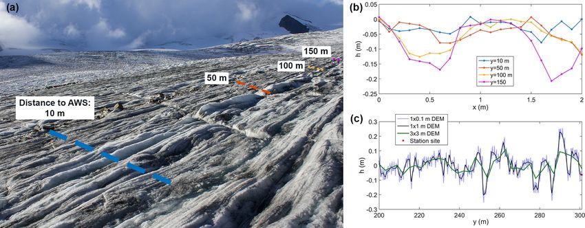
1054                                   N. Fitzpatrick et al.: A multi-season investigation of glacier surface roughness lengths

Figure 1. Location of the study glaciers and the stations installed during the 2014–2016 melt seasons.

Table 1. Locations and dates of operation of the automatic weather stations used in this study.

                    Station      NG14              CG15-1             CG15-2            CG16-1            CG16-2
                    Glacier      Nordic            Conrad             Conrad            Conrad            Conrad
                    Location     51.43434◦ N       50.82486◦ N        50.82306◦ N       50.82303◦ N       50.78219◦ N
                                 117.69973◦ W      116.92247◦ W       116.92128◦ W      116.91992◦ W      116.91197◦ W
                    Zone         ablation          ablation           ablation          ablation          accum.
                    Elevation    2208 m            2138 m             2163 m            2164 m            2909 m
                    Deployed     12 Jul 2014       15 Jul 2015        16 Jul 2015       19 Jun 2016       16 Jun 2016
                    Removed      28 Aug 2014       05 Sep 2015        07 Sep 2015       28 Aug 2016       22 Aug 2016

2.3    Lidar                                                             Nordic Glacier), while in 2015, the September flight over
                                                                         Conrad Glacier captured usable data for the accumulation
Airborne lidar was employed to obtain high-resolution to-                zone only.
pographic data over each of the study locations using a
Riegl 580 laser scanner and dedicated Applanix PosAV 910                 2.4     Data treatment
Inertial Measurement Unit. In general, flights were per-
formed over Nordic and Conrad glaciers twice per year (Ta-               2.4.1    Eddy covariance data
ble 3), close to the end of the winter and summer seasons
(April and September), as part of an ongoing mass balance                Prior to calculating observed values for the turbulent heat
survey of the study glaciers (Ben Pelto, unpublished data).              fluxes and roughness lengths, the raw (20 Hz) EC data were
By analysing the altimetry data from these times of the year,            passed through a series of preprocessing steps using the Ed-
it was hoped that the variation in surface roughness due to              dyPro data package (LI-COR, 2016). These steps are de-
the transition from a snow-covered to bare ice surface could             scribed in detail in Fitzpatrick et al. (2017), but a summary
be captured. In addition, the repeat mapping of each loca-               of the main techniques is provided below. A planar fit co-
tion from one year to the next would help identify the per-              ordinate rotation method (Wilczak et al., 2001) was applied
sistence in surface roughness. In 2014, April flights were not           to all of the sonic anemometer data to account for misalign-
performed over the glaciers (a July flight was performed over            ment of the z axis of the sensor with the w component of the

The Cryosphere, 13, 1051–1071, 2019                                                               www.the-cryosphere.net/13/1051/2019/
N. Fitzpatrick et al.: A multi-season investigation of glacier surface roughness lengths                                                           1055

Table 2. Instrument list for each deployed station, including sensor accuracy and heights of installation of the EC and temperature sensors
(z), and the wind monitor (zu ).

 Variable                         Sensor                                     Accuracy                      NG14      CG15-1   CG15-2   CG16-1   CG16-2
 Wind speed/direction             Young 05103ap Wind Monitor                 ±0.3 m s−1                         •         •        •        •        •
 Air temperature/humidity         Rotronic HC2 Probe                         ±0.1 ◦ C/0.8 %                     •         •        •        •        •
 Air temperature/humidity         Aspirated Rotronic HC2 Probe               ±0.1 ◦ C/0.8 %                     –         –        –        •        •
 Atmospheric pressure             Vaisala PTB110                             ±0.3 hPa                           •         •        •        •        •
 Precipitation                    Texas Elec. Tipping Bucket Gauge           ±1 % (up to 10 mm h−1 )            •         •        •        •        •
 Radiation fluxes                 Kipp & Zonen CNR4                          10–20 W m−2 (pyranometer)          •         •        •        •        •
                                                                             5–15 W m−2 (pyrgeometer)
 Turbulent fluxes:                OPEC System
    water vapour                     CSI IRGASON                             3.5 × 10⁻³ g m−3
    3-D wind (u, v, w)               CSI IRGASON                             1 mm s−1                           •         •        –        •        –
    sonic temperature                CSI IRGASON                             ±0.025 ◦ C
 Turbulent fluxes:                CPEC System
    water vapour                     LI-7200                                 ±2 %
    3-D wind (u, v, w)               Gill R3-50                              < 1 % rms                          –         •        •        •        •
    sonic temperature                Gill R3-50                              ±0.1 ◦ C
 Ground heat flux                 Thermistor array (self)                    ±0.1 ◦ C                            •        •        •        •        •
 Surface height                   CSI SR50A Sonic Ranger                     ±0.01 m                             1        3        3        3        3
 Surface temperature              Apogee SI-111                              ±0.2 ◦ C                            –        1        1        2        2
 Station tilt                     Turck Inclinometer                         ±0.5◦                               •        •        •        •        •
 Data storage                     CSI CR3000 Logger                          –                                   •        •        •        •        •
 Site/surface conditions          Time lapse camera (self)                   –                                   •        •        •        •        •
 z (m)                            –                                          –                                 2.0      2.0      2.0      1.9      1.9
 zu (m)                           –                                          –                                 2.6      2.5      2.6      2.6      2.4

Table 3. Dates of lidar flights over the two study glaciers from 2014                    2.4.2    Lidar data
to 2016.
                                                                                         The trajectories of each lidar flight had been previously post-
                  Nordic Glacier                       Conrad Glacier
                                                                                         processed using a network of permanent GPS base stations in
            Spring         Autumn               Spring        Autumn                     British Columbia. The positional uncertainties of the flight
  2014      10 July        11 September         –             11 September
                                                                                         trajectories were typically better than 5 cm, with the total
  2015      19 April       11 September         20 April      12 September∗              uncertainty in the processed lidar point clouds better than
  2016      17 April       12 September         17 April      12 September               ±10 cm, while the average point density for the lidar sur-
∗ For the 12 September 2015 flight over Conrad Glacier, only the accumulation zone
                                                                                         veys over the ice-covered terrain was 1–2 laser shots per
was adequately captured.                                                                 m2 (Ben Pelto, unpublished data). LAStools (Isenburg et al.,
                                                                                         2006) was utilised to classify the lidar data into ground and
                                                                                         non-ground laser returns. The ground returns were subse-
mean airflow. For the OPEC water vapour measurements, the                                quently gridded into DEMs with a 1 m2 grid cell, with the
Webb–Pearman–Leuning correction (Webb et al., 1980) was                                  grid lines aligned with true north and east.
used to correct for the density effects of air temperature fluc-
tuations, while readings from periods affected by precipita-                             2.5     In situ roughness length values
tion on the analyser windows were removed. These correc-
tions were not required for the CPEC water vapour data. The                              Roughness length values were calculated by implementing
turbulence data were averaged over 30 min blocks, and the                                EC data into the bulk method, with separate values calculated
calculated fluxes were filtered using quality tests for steady                           for OPEC and CPEC systems when both sensors were used
state and developed turbulent conditions, following Mauder                               at the same station:
and Foken (2004). Random error in the turbulent fluxes due
to sampling errors was estimated following the methods of
                                                                                                          uec          z
Finkelstein and Sims (2001). The mean random error over                                  z0v_ec = exp −κ      − ψm           z,                      (1)
all periods was ±4.5 W m−2 (9 %) for QH , and ±4.7 W m−2                                                 u∗ec         Lec

(15 %) for QL .                                                                                          Tec − Ts         z
                                                                                         z0t_ec = exp −κ          − ψh          z,                   (2)
                                                                                                           θ∗ec          Lec

                                                                                                         qec − qs         z
                                                                                         z0q_ec = exp −κ          − ψh          z,                   (3)
                                                                                                           q∗ec          Lec

www.the-cryosphere.net/13/1051/2019/                                                                            The Cryosphere, 13, 1051–1071, 2019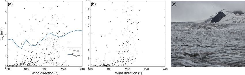
1056                                  N. Fitzpatrick et al.: A multi-season investigation of glacier surface roughness lengths

where κ is the von Kármán constant (0.4), z is the sensor             populate z0v and z0s . The values of the empirical coefficients
height, and uec , Tec , qec , u∗ec , θ∗ec , and q∗ec are the 30 min   (b0 , b1 , and b2 ) change for smooth (R∗ ≤ 0.135), transitional
EC-observed values for mean wind speed, air temperature,              (0.135 < R∗ < 2.5), and rough (R∗ ≥ 2.5) flow regimes, and
specific humidity, friction velocity, and the surface layer           between models.
scales for temperature and specific    humidity, respectively
                                                                      2.6     Remote momentum roughness length estimation

(Conway and Cullen, 2013). ψm Lzec and ψh Lzec are the
vertically integrated stability functions for momentum and            The set of 1 × 1 m grid cell DEMs obtained for the study
heat (Beljaars and Holtslag, 1991; Dyer, 1974), where Lec             glaciers from the lidar data were utilised to remotely estimate
is the Monin–Obukhov length. Glacier surface specific hu-             momentum roughness length values. Estimates were deter-
midity qs is calculated from atmospheric pressure p, and the          mined at the location of each station using the DEMs from
surface vapour pressure (es ), which is assumed to be at sat-         the same year the station was in place and compared with
uration at the glacier surface temperature (qs = 0.622es /p).         the EC-derived z0v_ec values. September DEMs were used to
To minimise potential errors and to obtain roughness lengths          estimate roughness length values for bare ice surfaces and
representative of the conditions at each site, an extensive se-       April DEMs for snow-covered surfaces (both the April and
ries of filters were applied to the 30 min values (see Fitz-          September DEMs at CG16-2 in the accumulation zone repre-
patrick et al., 2017, for full details). These filters included       sent a snow-covered surface). The DEM for Nordic Glacier
a 90◦ wind direction window centred on the main axis of               in July 2014 was used to estimate roughness lengths for the
the EC sensor (to minimise the influence of flow distortion           transitional snow-ice surface at NG14. The estimation of z0v
due to the station structure), minimum values for wind speed          was also repeated on DEMs from periods without a station
(> 3 m s−1 ) and u∗ec (> 0.1 m s−1 ), minimum differences             present at that location to allow for an examination of the
between measurement and surface height values of air tem-             temporal variation of roughness properties at each site over
perature (> 1 ◦ C) and vapour pressure (> 66 Pa) (Calanca,            the 3 years. Two methods were developed in this study, re-
2001; Conway and Cullen, 2013), a minimum scalar rough-               ferred to as the (i) block and (ii) profile methods. Both meth-
ness length value of 1 × 10⁻⁷ m based on the mean free path           ods assume that a DEM with a 1 × 1 m grid cell can ade-
length of molecules (Li et al., 2016), and a precipitation fil-       quately resolve the scale of the surface features that have the
ter. A test for stationarity of the turbulence, following Fo-         primary influence on roughness length. Where airflow en-
ken (2008), was also applied. This involved comparing each            counters a dense distribution of roughness elements (as can
30 min flux value with the average of the six 5 min flux values       be present on an ablating glacier surface), the flow is likely to
calculated within the same period. Turbulence for periods in          experience wake interference or skimming (Wieringa, 1993),
which the difference between these two values was greater             reducing the relative influence of smaller-scale roughness
than 30 % was deemed to be non-stationary, and these peri-            features on z0v (Smeets et al., 1999) and increasing the influ-
ods were excluded from the roughness length calculations.             ence of elements that are potentially resolvable at the DEM
The cut-off percentage was varied between 10 % and 50 % to            scale.
test the sensitivity to this selection. Finally, only roughness          Both methods draw on the empirical theory of Let-
length values calculated during near-neutral stability condi-         tau (1969) for the estimation of z0v from microtopography
tions (−0.1 < Lzec < 0.2) were retained to minimise the un-           measurements:
certainty associated with the stability functions applied in                        s
Eqs. (1)–(3) during non-neutral conditions (Smeets and van            z0v = 0.5h∗ ,                                                 (6)
                                                                                    S
den Broeke, 2008; Conway and Cullen, 2013).
                                                                      where h∗ is the average effective height of the roughness el-
Scalar roughness length modelling                                     ements above the surface, s is the average crosswind silhou-
                                                                      ette or face area of the roughness elements encountered by
The scalar roughness lengths from Eqs. (2) and (3) were               oncoming airflow, S is the lot area, equal to the total area of
compared with values from the surface renewal models of               the site divided by the number of roughness elements on its
Andreas (1987) and Smeets and van den Broeke (2008),                  surface, and the value 0.5 represents an average drag coeffi-
where the ratio of the scalar (z0s ) and momentum rough-              cient. The original application of the above theory assumes
ness lengths are expressed as a function of the roughness             that the surface is composed of regularly spaced roughness
Reynolds number R∗ :                                                  elements of similar size and shape, an assumption that may
      u∗ z0v                                                          not always hold for a glacier surface.
R∗ =         ,                                        (4)
    ν
    z0s                                                               2.6.1    Block estimation
ln        = b0 + b1 ln (R∗ ) + b2 ln (R∗ )2 .         (5)
    z0v
                                                                      The first method developed in this study to estimate z0v
ν is the kinematic viscosity of air (1.5 × 10⁻⁵ m2 s−1 ), and         aimed to account for the variation in shape and distribution of
the EC-derived roughness lengths (Eqs. 1–3) were used to              roughness elements on a glacier surface. First, the form drag

The Cryosphere, 13, 1051–1071, 2019                                                       www.the-cryosphere.net/13/1051/2019/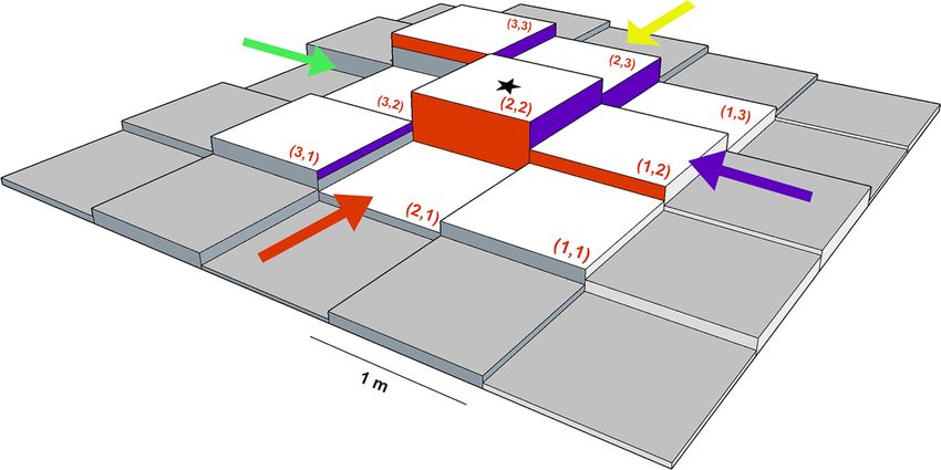
N. Fitzpatrick et al.: A multi-season investigation of glacier surface roughness lengths                                         1057

generated by the features on an individual portion or block            To estimate a momentum roughness length value at the
of the surface was estimated before combining the influence         location of a station, the effective influence of the FD_local
of each portion over a footprint to determine the momen-            values over the entire footprint must be determined. The flux
tum roughness length value for a given downwind location.           footprint of the turbulence observed at each station was es-
Similar methods were proposed and evaluated by Kondo and            timated using the model by Kljun et al. (2015). This model
Yamazawa (1986) for estimating z0v over irregular surfaces.         involves a two-dimensional parameterisation of a more com-
To account for the often dense distribution of roughness ele-       plex, backward Lagrangian particle dispersion model (the
ments on a melting glacier surface and the effects of this dis-     LPDM-B model in Kljun et al., 2002). In the above study,
tribution on airflow, the block method developed here also          the parameterisation was developed and evaluated for a wide
considers the relative height differences and potential shel-       range of boundary layer conditions and surface types and was
tering influence of neighbouring features on the surface.           shown to agree with the footprint estimates of the more com-
   As the method would be evaluated using roughness mea-            plex model. To estimate the footprints for the glacier stations
surements derived from the EC systems, it was applied to            in this study, EC-observed values for mean wind speed and
subareas of each DEM that contained the potential turbulent         direction, z0v_ec , Lec , u∗ec , and the standard deviation of lat-
footprint for a given station. Each subarea was 2000×2000 m         eral wind velocity were implemented into the parameterisa-
in dimension and centred on the grid cell containing the sta-       tion. Flux footprint maps were generated from the model,
tion site. For each grid cell in the subarea, a one-cell-thick      with a 1 × 1 m grid cell and total area of 2000 × 2000 m,
border was selected around the cell of interest, creating a         centred on the station location, to match the selected DEM
3 × 3 m block of cells (Fig. 2), representing a roughness ele-      subareas. Each grid cell was assigned a flux footprint value
ment and its surrounding area of influence. A localised drag        (fc ), representing its normalised contribution to the turbulent
value (FD_local ) was estimated for each block by utilising         flux observed at the station. Maps were generated for every
Eq. (6) and building on the methods of Smith et al. (2016).         30 min period in the EC data, from which an average seasonal
The heights of the cells in the block were detrended for the        footprint for the station was determined. For stations with
mean slope of the glacier in the region of the station, as it       two EC systems, separate footprint maps were generated for
was assumed that the mean airflow was parallel to this plane.       each to investigate sensitivity to the observation method.
The height values within the block were normalised, and the            The seasonal flux footprint map for a given station (or EC
mean height of all the cells above the zero plane was as-           system) was overlaid on the corresponding FD_local values
signed to h∗b . A value for sb was calculated for each cardi-       for the wind direction of interest. The FD_local value for each
nal wind direction, as follows. The heights of the first line of    grid cell was then weighted by its flux footprint contribution
cells in the block perpendicular to the oncoming wind (hi1          and summed over the subarea to obtain z0v_bloc :
e.g. heights of cells (3,1) (2,1), and (1,1) for the red wind
                                                                                 n
direction in Fig. 2) set the base levels for the silhouette area                 X
                                                                    z0v_bloc =         FD_locali fci ,                             (9)
in each row, and the maximum heights of the cells in each
                                                                                 i=1
row (e.g. heights of cells (3,3), (2,2), and (1,2)) set the upper
levels for the silhouette area. The sum of the silhouette areas     where n is the number of grid cells in the subarea. This pro-
of each row was then assigned to the sb value for that block        cess was then repeated for the DEMs available from each sea-
and wind direction:                                                 son. Standard error propagation methods were used to calcu-
       n                                                            late the uncertainty in z0v_bloc by considering the uncertain-
       X
sb =

             max hij − hi1 ,                                 (7)    ties in the lidar height data (< ±0.1 m) and the normalised
       i=1                                                          mean square error in the fc values from the footprint model
                                                                    (0.48; Kljun et al., 2015).
where n is the number of rows. The area of the block was               The primary application of a remote technique to estimate
assigned to the value for Sb . FD_local values were then calcu-     momentum roughness lengths would be to obtain values for
lated for each of the four cardinal wind directions for each        where in situ observations are not available, and therefore,
grid cell; the block in Fig. 2 shifting by one cell each step:      where the turbulent flux footprint for a given site is unknown.
                    sb                                              z0v_bloc values were first calculated with EC-derived foot-
FD_local = 0.5h∗b      .                                     (8)    prints, as above, to evaluate the effectiveness of the local
                    Sb
                                                                    form drag estimation (Eq. 8). To test the performance of the
A range of border thicknesses around each grid cell, from           block method in situations when EC data are not available,
one to five cells (3 × 3 to 11 × 11 m block area), was also im-     the observed turbulent footprints were then replaced with a
plemented to test the performance sensitivity to this choice.       series of assumed footprint areas at each site and applied to
Specifically, changing the border thickness represented a           the corresponding FD_local values to calculate z0v_bloc . The
change in the assumed size of the dominant roughness ele-           area of the assumed footprints ranged between 51 × 51 and
ments influencing z0v on the glacier surface and the assumed        251 × 251 m in size and was located directly upwind of the
range of a feature’s shadowing effect.                              station grid cell. The FD_local values for each cell within these

www.the-cryosphere.net/13/1051/2019/                                                           The Cryosphere, 13, 1051–1071, 2019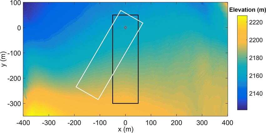
1058                                    N. Fitzpatrick et al.: A multi-season investigation of glacier surface roughness lengths

Figure 2. DEM-based block method for estimating the local drag generated by roughness elements on the surface. The total surface area that
is perpendicular and “visible” to the direction of airflow (matching-coloured face area and arrows) is assigned to sb (Eq. 7). The displayed
grid cell indices are for airflow in the direction of the red arrow. A FD_local value is estimated for the four cardinal wind directions, with the
values assigned to the central grid cell of the block (starred). The block is then moved by one grid cell at a time and the process is repeated
over the DEM.

areas were given an equal weighting and used to calculate a                for CG16-1 in September 2016. In this case, a separation
momentum roughness length value.                                           of scales was visually identified at a wavelength of approx.
                                                                           35 m, where the power spectrum was at zero. This value was
2.6.2   Profile estimation                                                 then used as a cut-off wavelength (λ0 = 35 m) to differenti-
                                                                           ate between large and small-scale surface features. With λ0
                                                                           identified, a fast Fourier transform (FFT) high-pass filter was
The second method developed in this study takes a profile-
                                                                           applied to the detrended profile to remove the large wave-
based approach to estimating momentum roughness lengths
                                                                           lengths (Fig. 3b) and to obtain a filtered profile. The filter-
and aims to identify the length scales relevant to form drag
                                                                           ing was performed in the wave number (k) domain with the
over that surface profile, rather than using the element by ele-
                                                                           following steps: (i) FFT was applied to the detrended profile
ment approach of the previous technique. Again, this method
                                                                           h(y) in Fig. 3b to get H (k), (ii) H (k) was modified by setting
is based on the theory of Lettau (1969), which is similar
                                                                           its values to zero for k < 2π/λ0 , and (iii) an inverse FFT was
to roughness estimation techniques used in previous stud-
                                                                           applied to the modified H (k) to get the filtered profileh(y) in
ies (e.g. Munro, 1989). Where it differs is in its application
                                                                           Fig. 3d. Finally, a value for momentum roughness length for
of this theory to wind-parallel profiles of the surface rather
                                                                           the filtered profile (z0v_prof ) was estimated through an appli-
than wind-perpendicular profiles. As with the block method,
                                                                           cation of the theory of Lettau (1969):
the first step was to detrend the surface height values for the
mean slope of the glacier. Beginning with roughness estima-
tion for the downslope (southerly) wind direction, a profile of                         σh s
                                                                           z0v_prof =        .                                               (10)
grid cells was selected from a given DEM along the glacier                               S
slope, which was 600 m in length, one grid cell wide, and
                                                                           S was calculated as the width of the profile (w = 1 m) mul-
centred on the location of a station. A linear trend was fit-
                                                                           tiplied by the length of the fetch (LF ) upwind of the station.
ted to this profile to identify the slope, and the trend was
                                                                           A range of values for LF were applied from λ0 to 2λ0 in 1 m
then removed from the original height data (Fig. 3a–b). This
                                                                           increments. The height of the grid cells along a given fetch
step was repeated for 50 parallel profiles on either side of the
                                                                           was assigned to an array from h0 to hN , where N is the num-
central “station” profile (101 profiles, in total). The next step
                                                                           ber of grid cells in the fetch, and the standard deviation of the
was to determine the scale of the features relevant to form
                                                                           height array along LF was assigned to σh :
drag, that is, the features that act as obstacles to airflow, and
to remove large-scale surface features or waves which air-                       v
                                                                                 uX h j − h 2
                                                                                 uN
flow may follow rather than be impeded by. The power spec-                 σh =  t                  .                                  (11)
trum was calculated for the detrended profile and analysed to                       j =0
                                                                                            LF
detect a separation of scales between large and small wave-
length features. In Fig. 3c, an example of the mean power
spectrum over 101 detrended profiles is shown in log–log

The Cryosphere, 13, 1051–1071, 2019                                                               www.the-cryosphere.net/13/1051/2019/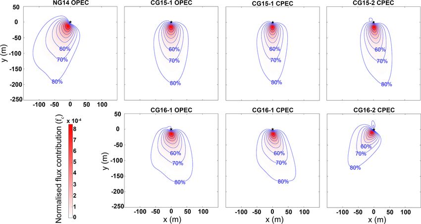
N. Fitzpatrick et al.: A multi-season investigation of glacier surface roughness lengths                                                1059

Figure 3. (a) Surface height profile from the September 2016 DEM centred on CG16-1 (red diamond) and a fitted linear trend; (b) detrended
profile and low-pass filter according to cut-off wavelength of λ0 ; (c) log–log power spectrum of the mean detrended profile, with large-scale
wavelengths greater than λ0 (green dashed line) used in the low-pass filtering; (d) filtered profile used in the calculation of momentum
roughness length.

A value for s was obtained from the sum of the height differ-
ences between adjoining grid cells:
        N
     wX
s=          hj − hj −1 ,                                       (12)
     2 j =1

with division by 2 to account for absolute height differences
above the mean height only. The mean of the calculated
roughness values from LF = λ0 to 2λ0 was then assigned to
the momentum roughness length for the station grid cell.
   To examine roughness length variability in the vicinity of
the station grid cell and to determine the uncertainty in the            Figure 4. Example of the rotation applied to a DEM patch selected
presented results, the above process was repeated for all grid           around a station location (red diamond), with the original orienta-
cells in the 101 × 101 m area upwind of the station (i.e. 50 m           tion, outlined in black, and a rotated patch turned 30◦ clockwise,
either side of the station profile). The profile method was              outlined in white.
also applied over a range of angles in addition to the pre-
vailing downslope, southerly direction, to examine the effects
of changing wind direction on momentum roughness length                  was created using data from microtopography profile mea-
(Fig. 4). To do so, the x–y grid matrix of a patch of grid cells         surements obtained at CG16-1 at the end of the melt season.
(101 m wide and 351 m long, containing the station site) was             Four surface height profiles, 2 m in length and with 0.1 m res-
multiplied by a rotation matrix (in 5◦ increments between 90             olution, were obtained at distances of 10, 50, 100, and 150 m
and 270◦ ). The height values from the DEM grid cells were               upwind of the station (Fig. 5a). The profiles were taken per-
then bilinearly interpolated to the rotated grid to derive new           pendicular to the prevailing wind direction (downslope) and
rotated height values. A value for z0v_prof was then calculated          measured using a 2 m snow probe, horizontally laid on the
as above for profiles in line with the long axis of the patch,           surface and allowed to partially melt in place. The long axis
and this was repeated for each 5◦ increment in rotation.                 of the probe was set as the zero plane, and the height of the
   The sensitivity of the profile method to the use of a DEM             surface was measured relative to this level at 0.1 m spacings.
with a finer (1×0.1 m) or coarser resolution (3×3 m) than the            Height variability parallel to the downslope direction was
original 1 × 1 m DEM was tested. As a 1 × 0.1 m DEM could                expected to be smaller than in the perpendicular direction,
not be derived from the lidar data, a synthetic test surface             which crosscuts supraglacial channels on the surface. There-

www.the-cryosphere.net/13/1051/2019/                                                             The Cryosphere, 13, 1051–1071, 2019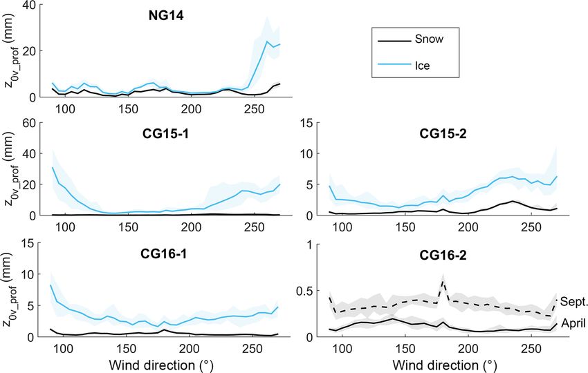
1060                                   N. Fitzpatrick et al.: A multi-season investigation of glacier surface roughness lengths

Figure 5. (a, b) Microtopography profiles taken upwind of CG16-1 at the end of the 2016 melt season. Profiles were 2 m in width and taken
perpendicular to the downslope direction. The locations of the profiles marked in panel (a) are representative rather than exact. (c) Examples
of the filtered height profiles, as derived from the three DEM resolutions and used in the z0v_prof sensitivity test.

fore, in the absence of microtopography measurements in                  log-normal. To present mean EC-derived values in the re-
this direction, the profile from the cross-slope direction with          mainder of this study, geometric means are used to avoid ex-
the smallest variance, i.e. the 10 m upwind profile (Fig. 5b),           cessively weighting the larger roughness values (Andreas et
was used to represent the slope-parallel variance. The mean              al., 2010). Stable atmospheric conditions persisted over the
was removed from this 2 m profile at a 1 m interval and lined            glaciers for much of each season, limiting the number of suit-
up in a repeated sequence to obtain an extended (600 m long)             able 30 min periods for roughness calculation after applica-
synthetic microtopography profile. The final test profile was            tion of the filters discussed in Sect. 2.5 (number of available
constructed by adding this extended synthetic profile to the             measurements presented in Table 4). Turbulence was found
detrended profile in the downslope wind direction from the               to be non-stationary for 21 % of the time on average. Vary-
1×1 m DEM. The same synthetic profile was added to the de-               ing the cut-off percentage in the stationarity test (originally
trended profiles from each side of the station, at 1 m distance          30 %) between 10 % and 50 % led to a ±15 % difference in
apart, yielding the synthetic 1 × 0.1 m DEM. The 3 × 3 m                 the calculated roughness length values on average.
DEM was created by applying a 2-D smoothing of the orig-                    Across all test sites, z0v_ec had means of 2.3 and 1 mm
inal 1 × 1 m DEM, using a 3-point running mean in both x                 for ice and snow, respectively, while the scalar roughness
(easting) and y (northing) directions. The profile method was            lengths had mean values of 0.05 mm for z0t_ec and 0.11 mm
then applied to both the 1 × 0.1 and 3 × 3 m DEMs for the                for z0q_ec . Where OPEC and CPEC systems were used at
600 × 101 m area upwind (slope-parallel) of the station, us-             the same station, the OPEC system returned slightly larger
ing the same steps as outlined previously. The same threshold            mean z0v_ec values (2.8 and 1.4 mm, respectively). Mann–
wavelength, λ0 = 35 m, was used to filter the profiles. Fig-             Whitney U tests applied to the 30 min roughness values from
ure 5c displays examples of filtered profiles, h(y), as derived          CG15-1 rejected the null hypothesis that the z0v_ec values
from the three DEM resolutions.                                          from the OPEC and CPEC systems had the same distribution
                                                                         (p < 0.01), but the hypothesis could not be rejected for the
                                                                         scalar values (p > 0.5).
3     Results                                                               The ice z0v_ec values were within the expected range for
                                                                         moderately rough glacier ice (1–4.5 mm; e.g. Brock et al.,
3.1    EC-derived roughness lengths                                      2006). Where measurements were repeated in the same area a
                                                                         year apart (CPEC observations on CG15-2 and CG16-1), per-
The geometric means of the roughness length values calcu-                sistence in the mean ice roughness length values was noted
lated from each EC data set are presented in Table 4, with               (0.86±7.4 and 0.74±6.4 mm), with a failure to reject the hy-
separate z0v_ec values for periods with snow and ice surfaces.           pothesis of equal distributions (p = 0.16). Within a season,
Each of the observed 30 min roughness length data sets were              substantial variability was noted in the 30 min z0v_ec values
found not to have a normal distribution (using one-sample                for each ice surface (Fig. 6a) but with no evident trend in
Kolmogorov–Smirnov tests), but one that was approximately                z0v_ec due to changes in surface roughness over time. Mean

The Cryosphere, 13, 1051–1071, 2019                                                            www.the-cryosphere.net/13/1051/2019/
N. Fitzpatrick et al.: A multi-season investigation of glacier surface roughness lengths 1061
Table 4. Seasonal geometric means of the EC-derived roughness length values (±σ ) from the open- and closed-path systems for each station
site. z0v_ec values for periods with a snow-covered surface are written in bold font. The number of 30 min periods available for roughness
estimation (after filtering) is presented in square brackets.
(mm) NG14 OPEC CG15_1 OPEC CG15_1 CPEC CG15_2 CPEC CG16_1 OPEC CG16_1 CPEC CG16_2 CPEC
z0v 4.5 ± 28.8 [93] 3.8 ± 31.7 [206] 2.0 ± 19.2 [281] 0.9 ± 7.4 [417] 1.7 ± 11.7 [308] 0.7 ± 6.4 [429] 2.4 ± 16[312]
0.46 ± 3[16] 0.62 ± 5.1[114] 0.51 ± 2.3[138]
z0t 0.01 ± 0.1 [77] 0.01 ± 0.88 [181] 0.09 ± 0.81 [270] 0.03 ± 0.28 [390] 0.03 ± 0.23 [396] 0.05 ± 0.29 [546] 0.01 ± 0.07 [247]
z0q 0.001 ± 0.008 [16] 0.23 ± 1.5 [43] 0.28 ± 1.9 [17] 0.21 ± 3.1 [74] 0.02 ± 0.28 [194] 0.01 ± 0.19 [186] 0.01 ± 0.1 [38]
Figure 6. 30 min z0v_ec values as observed at (a) CG16-1 and (b) CG16-2. The dashed line represents the commonly assumed z0v values of
1 and 0.1 mm for ice and snow. At CG16-1, the surface transitioned to bare ice on day of year (DOY) 183.
momentum roughness lengths for snow were also within pre- 3.2 Momentum roughness length from lidar
viously observed values on glacier surfaces, with a partic-
ularly large mean value observed at CG16-2 in the accu- 3.2.1 Block method
mulation zone (2.4 ± 16 mm). Extensive variability was also
present in the 30 min z0v_ec values for CG16-2 (Fig. 6b),
FD_local maps were generated from lidar-derived DEMs us-
with a general increasing trend in roughness over the sea-
ing the block estimation method (Fig. 8a–b) for all avail-
son. Across all stations and seasons, substantial variability
able years and seasons and for each of the four cardinal
was noted in the mean scalar roughness lengths, with z0q_ec ,
wind directions. Substantial variation in FD_local was ob-
in particular, showing a range of 2.5 orders of magnitude.
served across each glacier surface, ranging from 10−4 m for
z0t_ec exhibited less variability (∼ 1 order of magnitude),
snow-covered grid cells to 10−0.5 m for large crevasses. Fig-
with similar mean values observed for CG15-2 and CG16-
ure 9 displays the seasonal turbulent flux footprint maps gen-
1 (0.03 ± 0.28 and 0.05 ± 0.29 mm) and a failure to reject the
erated using the model by Kljun et al. (2015) for each EC
null hypothesis of equal distributions (p = 0.11).
sensor deployment. In general, the fluxes were sourced from
The ratios of the 30 min EC-determined scalar roughness
regions to the south of each station, in line with the prevailing
lengths to z0v_ec were expressed as a function of R∗ using
downslope winds at each site. Over 80 % of flux contribution
the data from all stations and seasons (Fig. 7). These val-
came from an area within 200 m upwind of each station, with
ues were compared with the surface renewal models of An-
concentrated peak source regions 15–20 m upwind on aver-
dreas (1987) and Smeets and van den Broeke (2008). The
age. The flux footprints of each EC data set were merged with
seasonal mean ratios and R∗ were also compared with these
the corresponding FD_local maps (Fig. 8c), producing a se-
models. In general, the roughness ratios were shown to de-
ries of z0v_bloc values for each site. As stated, wind direction
crease with increasing R∗ , with substantial scatter in the
was predominately from the south during each station de-
30 min values. The seasonal mean zz0v0t
ratios were in line with
ployment, so the roughness estimates for this wind direction
the output of the Andreas (1987) model (r 0.81; p < 0.05),
z0q (Table 5) are used for comparison with the EC-derived val-
with greater scatter in the z0v values (r = 0.2), while both
ues. The influence of wind direction on the roughness length
sets of ratios were underestimated by the Smeets and van den
estimates is discussed in Sects. 3.3 and 4.1.3.
Broeke (2008) model.
The mean uncertainty in the z0v_bloc values, estimated
from propagation of the errors in the lidar and flux foot-
print values, was ±0.53 mm. Where OPEC and CPEC sys-
www.the-cryosphere.net/13/1051/2019/ The Cryosphere, 13, 1051–1071, 20191062 N. Fitzpatrick et al.: A multi-season investigation of glacier surface roughness lengths
Figure 7. Performance of the surface renewal models of Andreas (1987) and Smeets and van den Broeke (2008) for estimating the ratio of
(a) z0t and (b) z0q to z0v . The filtered 30 min (grey) and seasonal mean (red) ratios of the EC-derived roughness lengths and R∗ values are
shown for all seasons and EC sensors.
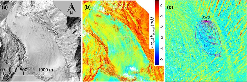
Figure 8. Example from CG16-1 of the steps taken to estimate z0v_bloc from lidar data: (a) 2000×2000 m subarea extracted from the 1×1 m
DEM, centred on an AWS; (b) localised drag values (FD_local ) calculated for each grid cell; (c) the flux footprint for the corresponding EC
data, shown as a percentage of crosswind integrated flux contribution (purple contours) and overlaid over the FD_local map (400 × 400 m
square area expanded from panel (b) for display purposes).
tems were used simultaneously on the same station (CG15-1 3.2.2 Profile method
and CG16-1), virtually identical z0v_bloc values were returned
when their flux footprints were applied. Therefore, only one The detrending and filtering of the surface height data, as
set of values is presented for each station in Table 5. Mean shown in Fig. 3, were performed for downslope profiles at
z0v_bloc values for ice and snow surfaces, over all sites and each station site using the DEMs for all available years and
seasons, were 3.1 and 0.6 mm, with strong persistence in site seasons. The same approximate value for the cut-off wave-
roughness values from one year to the next. A range of as- length (λ0 ≈ 35 m) was identified at each station site. z0v_prof
sumed footprint areas were also applied to the FD_local maps values were then estimated for each station location and for
to determine the effectiveness of the method in the absence of each grid cell in a 101 × 101 m upwind area (Fig. 10a), from
observed footprint data. Applying equal weighting to FD_local all corresponding DEMs. Table 5 presents the z0v_prof values
values in a 101×101 m area directly upwind of a site (fc_100 ) for each station and lidar flight. Mean z0v_prof values for ice
was found to return roughness values close to the z0v_bloc and and snow surfaces, over all sites and seasons, were 4.3 and
z0v_ec values, in most cases (Table 5). 1.1 mm. Where repeated over the same location, the z0v_prof
As previously stated, the sensitivity of roughness length values displayed substantial differences from one year to the
estimation to the selected block size was tested by varying next over ice surfaces (up to 5 mm), in contrast to the noted
the border thickness around the grid cell of interest. Overall, z0v_bloc persistence.
increasing the block area was found to lead to an increase in Figure 10b displays the z0v_prof values derived for the
estimated roughness length for a given footprint, with a bor- downslope profiles from the original DEM (1×1 m) and from
der thickness of 1 cell (3 × 3 m block area) returning rough- the higher- (1×0.1 m) and lower- (3×3 m) resolution DEMs
ness lengths closest to the EC-derived values at all stations constructed for sensitivity testing. Roughness values are pre-
(e.g. CG16-1 ice z0v_bloc = 1.6, 1.9, 2.0, 2.2, and 2.4 mm for sented for the station location at CG16-1 and for the grid cells
an increasing border thickness range of 1–5 cells). 50 m to the east and west of the station. The same pattern
of spatial variability in z0v_prof across the grid cells was cap-
The Cryosphere, 13, 1051–1071, 2019 www.the-cryosphere.net/13/1051/2019/N. Fitzpatrick et al.: A multi-season investigation of glacier surface roughness lengths 1063
Figure 9. Flux footprint maps for each EC system deployed during the study, including percentage of crosswind integrated flux contribution
(purple contours). Distances are in metres east (x) and north (y) of the AWS (black star). Maps were produced following the methods of
Kljun et al. (2015).
Table 5. Momentum roughness length values (in millimetres) for each station estimated using remote methods (z0v_bloc and z0v_prof ) from
the lidar-derived DEMs. The roughness values for the prevailing downslope southerly wind direction are shown here. fc_100 represents
values for an assumed 101 × 101 m upwind footprint, where FD_local values are given equal weighting. The uncertainty values from error
propagation are shown for z0v_bloc , while for z0v_prof , ±σ of the roughness values for the 101 × 101 m upwind patch is presented.
NG14 CG15-1 CG15-2 CG16-1 CG16-2
z0v_bloc April September April September April September April September April September
2014 – 6.3 ± 0.9 – 2.5 ± 0.1 – 2.5 ± 0.5 – 1.6 ± 0.4 – 0.5 ± 0.2
2015 2.0 ± 0.2 5.0 ± 0.1 0.3 ± 0.2 – 0.5 ± 0.2 – 0.3 ± 0.2 – 0.3 ± 0.1 0.4 ± 0.2
2016 2.5 ± 0.1 4.0 ± 0.4 0.6 ± 0.3 4.0 ± 0.4 0.8 ± 0.2 3.2 ± 0.5 0.3 ± 0.1 1.6 ± 0.5 0.4 ± 0.1 0.4 ± 0.1
fc_100 2.0 ± 0.2 3.2 ± 0.4 0.5 ± 0.2 4.2 ± 0.2 0.6 ± 0.2 2.1 ± 0.5 0.2 ± 0.1 0.9 ± 0.4 0.2 ± 0.1 0.2 ± 0.1
z0v_prof
2014 – 6.9 ± 0.3 – 2.6 ± 0.2 – 2.0 ± 0.3 – 2.1 ± 0.2 – 0.4 ± 0.02
2015 4.6 ± 0.4 4.2 ± 0.4 0.2 ± 0.04 – 0.5 ± 0.02 – 0.9 ± 0.03 – 0.1 ± 0.01 0.2 ± 0.04
2016 3.6 ± 0.2 5.6 ± 0.1 0.6 ± 0.1 5.6 ± 0.5 1.7 ± 0.1 7.1 ± 0.6 0.7 ± 0.03 2.6 ± 0.2 0.1 ± 0.02 0.6 ± 0.04
tured with each DEM but with substantial differences in mag- downslope wind direction in the 1 × 0.1 m DEM. To test for
nitude. On average, the 3 × 3 m DEM yielded z0v_prof values this, the amplitude of the synthetic microtopography profiles
1 order of magnitude smaller than the original 1 × 1 m DEM. was reduced by a factor of 10 (from decimetre to centime-
This result is expected since the original surface has been tre scale) and z0v_prof recalculated. The resulting roughness
smoothed, and the relevant scales of the roughness elements length values were reduced and matched the original z0v_prof
may not be adequately resolved in the 3 × 3 m DEM. When from the 1 × 1 m DEM more closely; however it still yielded
applied to the 1 × 0.1 m DEM, the profile method yielded up to 10 % larger values than the original (Fig. 10b).
roughness values that were on average 0.5 orders of mag-
nitude larger than those for the 1 × 1 m DEM. The primary 3.2.3 In situ vs. remote methods
reason for differences in z0v_prof values with changing DEM
resolution was the difference in s values (Eq. 12). While σh The estimates from both DEM-based roughness methods
values remained almost unaltered for different resolutions, (applied to a 1 × 1 m DEM) were compared with the EC-
the s values changed by > 50 %, resulting in large changes derived values (Fig. 11 and Table 6). In cases where lidar
in z0v_prof . data were not available from the same year a station was
The first-order estimate of surface variability from the mi- in place, the averages of the roughness estimates from the
crotopography survey may overestimate the variability in the 2 other years were utilised for the comparison. Overall, es-
www.the-cryosphere.net/13/1051/2019/ The Cryosphere, 13, 1051–1071, 2019You can also read