A new European land systems representation accounting for landscape characteristics - DORA 4RI
←
→
Page content transcription
If your browser does not render page correctly, please read the page content below
Landscape Ecol
https://doi.org/10.1007/s10980-021-01227-5
RESEARCH ARTICLE
A new European land systems representation accounting
for landscape characteristics
Yue Dou · Francesca Cosentino · Ziga Malek · Luigi Maiorano · Wilfried Thuiller ·
Peter H. Verburg
Received: 8 August 2020 / Accepted: 26 February 2021
© The Author(s) 2021
Abstract Methods Combining the recent data on land cover
Context While land use change is the main driver and land use intensities, we applied an expert-based
of biodiversity loss, most biodiversity assessments hierarchical classification approach and identified
either ignore it or use a simple land cover representa- land systems that are common in Europe and mean-
tion. Land cover representations lack the representa- ingful for studying biodiversity. We tested the ben-
tion of land use and landscape characteristics relevant efits of using this map as compared to land cover
to biodiversity modeling. information to predict the distribution of bird species
Objectives We developed a comprehensive and having different vulnerability to landscape and land
high-resolution representation of European land sys- use change.
tems on a 1-km2 grid integrating important land use Results Next to landscapes dominated by one land
and landscape characteristics. cover, mosaic landscapes cover 14.5% of European
terrestrial surface. When using the land system map,
species distribution models demonstrate substantially
Supplementary Information The online version of this
article contains supplementary material which is available
higher predictive ability (up to 19% higher) as com-
at (https://doi.org/10.1007/s10980-021-01227-5). pared to models based on land cover maps. Our map
consistently contributes more to the spatial distribu-
Y. Dou (*) · Z. Malek · P. H. Verburg tion of the tested species than the use of land cover
Environmental Geography Group, Institute
data (3.9 to 39.1% higher).
for Environmental Studies (IVM), Vrije Universiteit
Amsterdam, De Boelelaan 1087, 1081 HV Amsterdam, Conclusions A land systems classification includ-
The Netherlands ing essential aspects of landscape and land manage-
e-mail: yue.dou@vu.nl ment into a consistent classification can improve upon
traditional land cover maps in large-scale biodiversity
F. Cosentino · L. Maiorano
Department of Biology and Biotechnologies “Charles assessment. The classification balances data availabil-
Darwin”, University of Rome “La Sapienza”, Rome, Italy ity at continental scale with vital information needs
for various ecological studies.
W. Thuiller
Laboratoire D’Ecologie Alpine, LECA, Université
Grenoble Alpes, CNRS, Université Savoie Mont Blanc, Keywords Land system · Land management · Land
Grenoble, France use intensity · Biodiversity assessment · Species
distribution model · Large-scale
P. H. Verburg
Swiss Federal Institute for Forest, Snow and Landscape
Research (WSL), Birmensdorf, Switzerland
Vol.:(0123456789)
13
Landscape Ecol

Introduction                                               use and landscapes in empirical studies mostly by
                                                           land cover. This is a direct result of the relative
Landscape ecology envisions the landscape as               ease of observing land cover from remote sensing
the outcome of the complex relationship between            while land use intensity or land use management
humans and nature (Opdam et al. 2018). Land sys-           is more difficult to characterize and data are often
tem science defines land systems, similarly, as the        absent (Kuemmerle et al. 2013; Erb et al. 2017).
terrestrial component of the Earth system encom-           This is especially the case for larger scale assess-
passing all processes and activities related to the        ments (Verburg et al. 2013b). Rather than represent-
human use of land, including socioeconomic,                ing the landscape and its composition, the dominant
technological and organizational investments and           land cover is used to represent the land system and
arrangements (Verburg et al. 2013a). Land system           landscape. Some approaches use a representation
change is seen as both a cause and consequence of          that describes the different land cover fractions,
socio-ecological processes, rather than as a sole          but ignoring their spatial configuration. It is well-
outcome, or emergent property, of human–envi-              known that many of the Earth’s landscape are mosa-
ronment interactions (Verburg et al. 2015). Land           ics of different land covers, encompassing novel
system science and landscape ecology share a lot           ecosystems (Perring and Ellis 2013). Although
of concepts of interest: the acknowledgement of            coarse-scale land cover representations are always
human activities as a main actor of land use and           constrained in thematic resolution, ignoring these
landscape change (Lambin et al. 2001; Turner II            important mosaic landscapes is an important
et al. 2007; Roy Chowdhury and Turner 2019); the           omission.
importance of addressing multiple spatial and tem-            More recently land system representations have
poral scales (Veldkamp and Lambin 2001; Dear-              been proposed to better capture human use of the
ing et al. 2010); the attention for human benefits of      land, or some aspects of landscape configuration. For
nature through the concepts of ecosystem services          example, Ornetsmüller et al. (2018) distinguished
and Nature’s contributions to People (Wu 2013) and         permanent agricultural use from shifting cultiva-
the attention for sustainability solutions (Nielsen        tion in a land systems classification for Laos while
et al. 2019). At the same time, landscape ecologists       Debonne et al. (2018) represented smallholders vs
have been putting a strong emphasis on character-          large scale land acquisitions explicitly given their dif-
izing landscape pattern across spatial and temporal        ferent drivers and social and environmental impacts.
scales (O’Neill et al. 1988; Li and Wu 2004; Wu            On a global scale, Ellis and Ramankutty (2008) and
2004), and understanding how landscape structure           Václavík et al (2013) used a wide range of environ-
and composition emerge from socio-ecological pro-          mental and demographic conditions to identify arche-
cesses and impact the functioning and performance          typical combinations of socio-ecological conditions
of ecosystems (Nagendra et al. 2004). Land system          defining land use, while van Asselen and Verburg
science has, in contrast, often focused on the char-       (2012) used information on land cover, input inten-
acterization and explanation of land use change at         sity and livestock to subdivide global land cover into
the level of individual pixels (observed from remote       land systems. These land system representations have
sensing), plots or at the level of individual or collec-   been created for various purposes and, while mak-
tive actors (Overmars and Verburg 2006; Manson             ing the best use of available data, improved over land
2007), with less specific attention for the landscape      cover classifications by including specific aspects rel-
patterns and structures. Despite common analytical         evant to landscape ecology and land system science.
methods, these different foci can lead to different        However, in spite of this progress, most global assess-
representations of the landscape and its dynamics,         ments for biodiversity such as for IPBES and IPCC
having repercussions for interpretation and assess-        are still based on relatively rough and classical land
ment of drivers and impacts of land use and land-          cover representations.
scape changes.                                                In particular, most large-scale biodiversity mod-
   While both disciplines acknowledge the role             elling (especially those using species distribution
of human use of land, both often represent land            modelling, SDM) have so far either focused on the

13
Landscape Ecol

impacts of climate change (Thuiller et al. 2019)        management conditions. In this paper we aim to
or on climate change with some broad land cover         present a continental-scale land system classifica-
classes (Thuiller et al. 2014). This has been done      tion for Europe making best use of available data
in SDM by simple filtering species distributions by     that moves beyond the many assessments of biodi-
land cover classes (Maiorano et al. 2013; Powers        versity that are using rough land cover classes and
and Jetz 2019) or land use types (Newbold 2018).        relationships between land cover and habitat for
Another approach in biodiversity assessments is to      species (Newbold 2018; Powers and Jetz 2019). We
assign expert based values to land use, based on the    focus our analysis on including aspects of landscape
observed or expected effect it has on biodiversity,     structure and land use intensity. There is sufficient
or based on the level of naturalness (Pouzols et al.    evidence that land use intensity (Beckmann et al.
2014; Di Minin et al. 2016). Such approaches not        2019) and landscape structure (Walz and Syrbe
only require a well-established relationship between    2013; Boesing et al. 2017) are strong determinants
different species and the land use impact, but also     of the land use impact on biodiversity. Recent stud-
neglect some landscape characters and land man-         ies showed the impact of forest management types
agement that play important roles in biodiversity.      on species richness (Chaudhary et al. 2016) and the
While some large-scale biodiversity assessments         differences of accounting for forest management in
account for nitrogen application and habitat frag-      addition to forest cover change on global biodiver-
mentation as additional stressors (Schipper et al.      sity (Schulze et al. 2020). Other studies indicated
2020), these are independently addressed from land      the role of agricultural management (Beckmann
cover information without using an integrated land-     et al. 2019) and livestock grazing (Zhang et al.
scape approach.                                         2017; Li et al. 2019), as well as the importance of
    There were several reasons to ignore land use       landscape mosaic for conservation (Harvey et al.
or land cover in these models that relate species       2008) and ecosystem service provisioning (Dainese
occurrence (or abundance) to environmental vari-        et al. 2019). While land use studies often character-
ables. The first one was that since land cover and      ize urban area by the amount of build-up land (Seto
land use are mainly driven by climate, they do not      et al. 2012; van Vliet et al. 2019) the structure of
bring much additional information, and rather cre-      urbanization has a strong impact on biodiversity
ate some multi-collinearity issues when combined        (Malkinson et al. 2018). In peri-urban areas the
with climatic variables in SDMs (Thuiller et al.        build-up land cover is often not vast, but the wide-
2004). The second reason is that past land cover        spread disturbance through human activities and
or land use maps were generally of poor thematic        infrastructure causes much larger declines in bio-
resolution (e.g. forest, urban, cropland, grassland     diversity than the overall build-up area would sug-
and other) which prevent to estimate the tight asso-    gest (Buczkowski and Richmond 2012; Concepción
ciation that could arise between a given species and    et al. 2016).
for instance extensive croplands. Still, some recent       The land system typology presented in this paper
exercises have shown the interest of using detailed     aims at incorporating important elements of the land-
land use classification to predict species extinction   scape and land system relevant to biodiversity. To
at global scale (Powers and Jetz 2019). IPBES (Diaz     demonstrate the added value of such representation
et al. 2019) also identified land use change as the     compared to the often-used land cover classifications,
main driver of biodiversity loss and several papers     we used bioclimatic variables and the land system map
have argued for inclusion of land use change as         to model the species distribution on nine selected bird
part of biodiversity assessments (Titeux et al. 2016;   species that have wide habitat range across Europe
Randin et al. 2020).                                    with different vulnerability to land use and landscapes.
    A way to possibly advance large-scale biodiver-     We hypothesized that the predictive ability of models
sity assessments is to provide a land system clas-      and variable contribution to the spatial distribution is
sifications map that includes more ecologically         improved by the new land system typology.
relevant variables describing landscape and land

                                                                                                     13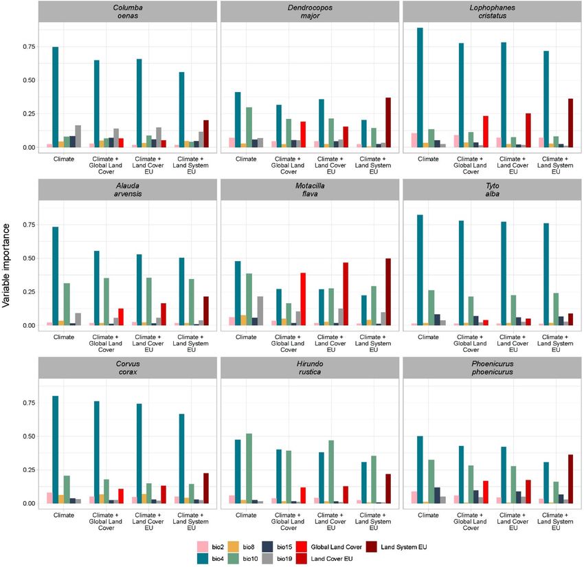
Landscape Ecol

Table 1  Overview of land systems
Land system           Subdivisions                            Description of systems

1. Settlement sys-    1.1 Low-intensity settlement            Low-medium density, far away from urban cores
  tems                1.2 Medium-intensity settlement         Medium density or adjacent to urban core
                      1.3 High-intensity settlement           High imperviousness
2. Forest systems     2.1 Low-intensity forest                High probability as primary forest and low/medium wood production
                      2.2 Medium-intensity forest             Low probability as primary forest and medium wood production
                      2.3 High-intensity forest               Low probability as primary forest and high wood production
3. Cropland systems   3.1 Low-intensity arable land           Low inorganic fertilizer input, small field size
                      3.2 Medium-intensity arable land        Medium inorganic fertilizer input, medium field size
                      3.3 High-intensity arable land          High inorganic fertilizer input, large field size
                      3.4 Low-intensity permanent crops       Vineyards, olive graves, fruit gardens, with understory vegetation,
                                                               this class also has mixed annual and permanent crops
                     3.5 High-intensity permanent crops       Vineyards, olive graves, fruit gardens, without understory
4. Grassland systems 4.1 Low-intensity grassland              Low density of livestock, low inorganic fertilizer input, and low
                                                               mowing frequency
                      4.2 Medium-intensity grassland          Medium density of livestock, medium use of inorganic fertilizer, and
                                                               medium mowing frequency
                      4.3 High-intensity grassland            High density of livestock, high inorganic fertilizer input, and/or high
                                                               mowing frequency
5. Shrub                                                      Areas dominated by shrub land cover or similar
6. Rocks and bare                                             Areas dominated by rocks, bare soil, or similar
  soil
7. Mosaic systems     7.1 Forest/shrub and cropland mosaics   Areas with small parcels of forest/shrubs and cropland
                      7.2 Forest/shrub and grassland mosaic   Areas with small parcels of forest/shrubs and grassland
                      7.3 Forest/shrubs and bare mosaics      Areas with small parcels of forest/shrubs and bare land
                      7.4 Forest/shrubs and mixed agricul-    Areas with small parcels of forest/shrubs and mixed areas of cropland
                        ture mosaics                           and grassland
                      7.5.1 Low-intensity agricultural        Low density of inorganic fertilizer input, small field size, and low
                        mosaic (cropland and grassland)        livestock density
                      7.5.2 Medium-intensity agricultural     Medium use of inorganic fertilizer, medium field size, and medium
                        mosaic (cropland and grassland)        livestock density
                      7.5.3 High-intensity agricultural       High inorganic fertilizer input, large field size, and/or large livestock
                        mosaic (cropland and grassland)        density
8. Snow, water,       8.1 Glaciers                            Areas dominated by glaciers, wetland, or water body
  wetland systems     8.2 Water body
                      8.3 Wetland

Materials and methods                                               the following major land systems groups (Table 1):
                                                                    water and wetland systems, human settlement sys-
Classification overview                                             tems, forest systems, grassland systems, cropland
                                                                    systems, and mosaic systems. These land systems
We used an expert-based land system classification                  are selected based on common land uses in Europe,
approach based on variables for which there is evi-                 are represented by major groups in the continent’s
dence of the effect on biodiversity. We operation-                  land use and land cover datasets (ESA and UCLou-
alized land systems as areas that host one or more                  vain 2010; European Environment Agency 2018) and
land use activities at the landscape level having an                by expert opinions towards their importance to study
impact on species occurrence and biodiversity. We                   the impacts of land use on biodiversity. Particularly,
focused, consistent with traditional classifications, on            the inclusion of mosaic system and the separation

13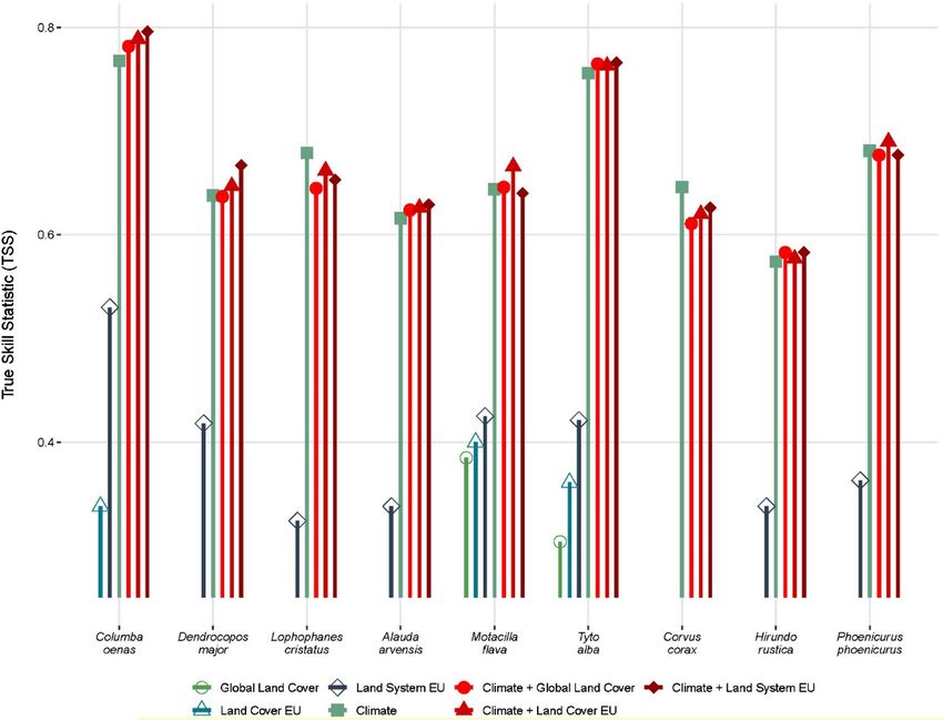
Landscape Ecol

of forest mosaics and agricultural mosaics is aimed          We operated on a 1-km2 spatial resolution.
at better capturing the fragmented forest habitat and     Although some land cover data may have a more
agricultural composition that certain forest and agri-    detailed resolution (e.g., Corine at 100 m or Glob-
cultural species are sensitive to (García-Navas and       Cover at 300 m), the pursuit for a finer resolution
Thuiller 2020). We also have permanent crops as           than 1-km2 is hampered by a lack of the high-reso-
a sub-system in the cropland category because they        lution data on land use intensity and management.
can provide vital habitat for certain species and the     Meanwhile, bio-climatic variables used for the large-
management styles for permanent crops can gener-          scale biodiversity assessment and species distribu-
ate distinctive biodiversity consequences (Bruggisser     tion modeling are derived from global interpolations
et al. 2010; Winter et al. 2018). The threshold of land   across the multitude of existing climatic stations.
cover extent for each land system was determined          These interpolations have been made at global scale
based on two criteria: it indicates the composition of    at 1-km2 and are provided from web portals like
land cover of the system (e.g., covers the majority of    WorldClim or CHELSA. Some species may be able
the pixel, or the mosaic combinations are meaning-        to thrive in habitat patches smaller than 1-km2, how-
ful for certain species), and it captures small habitat   ever this character, at least in some cases, can be cap-
area requirements. Residential systems also include       tured by the mosaic land systems that we represent in
those with relatively low fractions of build-up land as   our typology. Therefore, a spatial resolution of 1-km2
the impact of associated activities and infrastructure    is an optimal choice for this study, considering data
on species is often proportionally large (Buczkowski      availability and usage for biodiversity assessment.
and Richmond 2012; Concepción et al. 2016).These             We complied and harmonized data of land cover
land systems were further classified based on differ-     composition and intensity indicators using a Geo-
ent land use intensity indicators. We also aggregated     graphic Information System based approach. Data
classes with small areas (the full expert-based hier-     were chosen based on the following principles: (1)
archical classification procedure is included in Fig.     they are publicly available, (2) we prioritized the
S3). Our expert-based procedure, although tailored        highest spatial resolution and most recent date, (3)
to the European conditions and for use in biodiver-       data produced at the European scale have priority
sity assessments, follows common patterns with other      over global datasets, (4) if the data were a result of
global and regional land system classifications (e.g.     downscaling, we ensure that no co-variates are used
Ellis and Ramankutty 2008; van Asselen and Verburg        in the downscaling that would induce multi-colline-
2012; Herrero et al. 2014; Malek and Verburg 2017;        arity with other variables often used in biodiversity
Kikas et al. 2018).                                       modeling. (5) Global data were only used if previous
   We chose the spatial extent of the European Union      criteria cannot be achieved and data gaps are appar-
(EU) with the United Kingdom (EU28 +), Norway,            ent in particular regions. We mostly relied on global
Switzerland, and the Western Balkans (Serbia, Kos-        data for the non-EU region. All maps were resampled
ovo, North Macedonia, Montenegro, Albania, and            to a 1-km2 spatial resolution using the Lambert azi-
Bosnia and Herzegovina). However, we excluded             muthal equal-area projection that is frequently used
Iceland, Turkey and Europe’s Outermost regions and        for European maps. The details of data and methods
Overseas Countries (mostly islands not present on the     used for each system are discussed below (Overview
European continent) due to data issues, the analytical    see Tables 1, S3 and S4, Fig. S3).
interests, and their limited importance for assessing
continental species and biodiversity. To the best of      Extent of land systems
our knowledge, this is the most complete coverage of
land cover and land use analysis at the European scale    For land cover extent, we used Copernicus products
while most studies do not cover non-EU countries          derived from remote sensing data, such as CORINE
such as Switzerland, Norway, and the Balkans. Such        land cover 2018 (CLC) (European Environment
continuity of coverage is important for modeling spe-     Agency 2018) and Pan-European High Resolution
cies migration and projected changes due to climate       Layer (HRL) thematic maps (i.e., imperviousness,
change. We refer to this region as the non-EU region      forests, grassland, water & wetness) (European Envi-
and the other parts as EU region.                         ronment Agency 2015a, b, c, d). A global glacier

                                                                                                       13
Landscape Ecol
database was used for the extent of glaciers (Global Human settlement systems
Land Ice Measurements from Space (GLIMS) and
National Snow and Ice Data Center 2012) (Table S3). Urbanization in Europe undergoes multiple dimen-
We aggregated the HRL thematic maps from 20 m to sional changes in land cover, land use, and socio-eco-
1 km to derive the extent of (1) human settlement, (2) logical activities (Shaw et al. 2020), and most recent
forests, (3) water and wetlands, and (4) grasslands. changes are small incremental increases (van Vliet
For the remaining land covers, including croplands et al. 2019). In comparison to current practices that
(annual and permanent) and other land cover classes use “built-up” land or a binary classification of urban
(e.g., shrubs, bareland and rocks) we used CLC maps and rural area (Seto et al. 2012), we classified three
to resample. intensity levels for settlement systems: urban core
Classification thresholds based on the share of par- (high intensity), peri-urban (medium intensity), and
ticular land cover within the 1-km2 pixel were chosen villages (low intensity) based on the degree of imper-
based on expert opinions for each system (Table 1). viousness and spatial connectivity to urban core.
First, this enabled us to study land cover types that We used the intensity of imperviousness (i.e., each
may affect species largely but appear on a smaller cell has a value from 0 to 100%), namely artificial
scale, such as settlement systems. In addition, we impermeable cover of soil, as a proxy of urbanization
used indicators other than land cover composition degree, following similar mapping exercises (Linard
to characterize these classes, among which one par- et al. 2012; van Asselen and Verburg 2012; Demuzere
ticular example is the peri-urban and villages that et al. 2019). In addition, we considered the adjacency
may have less built-up land than cropland and forest to urban core areas when distinguishing peri-urban
cover (van Vliet et al. 2019). Despite the small per- and rural settlements (Linard et al. 2012; Stürck et al.
centage, these classes may cause profound effects on 2018) (Fig. S4).
species activities due to the continuity and irrevers-
ibility of human disturbances. Second, compared Forest systems
to most land cover classification that determines the
class by the largest land cover, we used a threshold Forest management and forest types are important to
of 70% to classify areas dominated by forest, crop- accurately assess biodiversity (Chaudhary et al. 2016;
land, and grassland. This is to better describe these Schulze et al. 2020). We used wood production of
classes with homogeneity while defining landscapes Europe (Verkerk et al. 2015) and the probability of
with several different land cover classes as mosaics. finding primary forest (Sabatini et al. 2018) to charac-
A pixel that contains multiple land cover components terize the intensity of forest use in the EU region (Fig.
smaller than 70% of the cell is classified as a mosaic S5). For the non-EU region, we extracted the forest
system, which is further subdivided by its main land classes from a global dataset (Schulze et al. 2019).
cover type. As we acknowledge that all these thresh- The three classes (i.e., primary, naturally regrown,
olds are arbitrary and set to balance the importance of and planted) were reclassified as low-intensity,
the land system components for biodiversity and the medium-intensity, and high-intensity to fit our forest
number of complex compound classes, we conducted classification (while acknowledging these classes do
a sensitivity analysis of the thresholds on the extent not fully correspond).
of land systems (Supplementary Material). We found
only small changes in the overall patterns of land sys- Grassland systems
tems upon changing the thresholds within reasonable
ranges. Three indicators were used to map the intensity of
grazing grassland: livestock unit density, nitrogen
Intensity of land systems input, and mowing frequency. We selected three
ruminant livestock groups (i.e., cattle, goat, and
We used a range of metrics to measure land use inten- sheep) from the global dataset on livestock density
sity and landscape characteristics (detailed intensity (Gilbert et al. 2018) and converted them to livestock
classification of each system can be found in the sup- unit (LSU) density (Eurostat 2013), which is the
plementary material). number of animals equivalent to one adult dairy cow
13Landscape Ecol
producing 3000 kg of milk annually (LSU/km2). The understory between stripes of grapes and olive trees
nitrogen application rate was calculated using a novel are an important indicator both for habitats and man-
downscaling of statistical data by the Joint Research agement styles (Bruggisser et al. 2010; Winter et al.
Center, which included mineral fertilizer input, the 2018). Therefore, the second land cover type identi-
manure application and deposition by grazing ani- fied in LUCAS (Eurostat 2018) was selected, repre-
mals. The indicator of mowing frequency represents senting the understory vegetation, as a biodiversity
the average number of annual mowing events in the relevant indicator of management intensity (Fig. S8).
period of 2000–2012 (Estel et al. 2018). The LSU
density and nitrogen application rates were reclas- Mosaic systems
sified into three levels as low, medium, and high.
This is based on the biodiversity dynamics relevant Pixels without dominant land cover types were clas-
to nitrogen application rate (Kleijn et al. 2009) and sified as mosaic systems. Two sub-mosaic systems
supported by other studies (van der Zanden et al. were classified: agricultural mosaics and forest/shrubs
2016; Estel et al. 2018). When combining the three mosaics. Croplands and grasslands without tree cover
indicators, LSU was used as the primary indicator were aggregated to agricultural mosaic systems. This
and then complemented by nitrogen and finally the sub-system was further classified into three agricul-
mowing frequency (Fig. S6). For the non-EU region, tural intensities: low, medium, and high. Two indica-
we could only use LSU as the indicator due to data tors, LSU and nitrogen application rate from the same
unavailability. source as above, were used. LSU was used as the pri-
mary indicator and nitrogen was the secondary indi-
Cropland systems cator (Fig. S9).
The forest/shrub mosaics include mixed land
Erb et al. (2013) and Kuemmerle et al. (2013) inven- cover types with some portion of forest/shrubs. This
toried the conceptual basis of cropland intensity and is because forest fragments, remnant trees, and small
provided a range of potential input and output indi- parts of shrubs and bare can serve as valuable habi-
cators. We focused on agricultural input alone, and tats for many species. These mixed compositions
chose nitrogen input and field size as indicators with increase landscape connectivity and preserve poten-
high relevance for many species, to quantify the agri- tial for restoration (Harvey et al. 2008; Horák et al.
cultural intensity. 2019). Forest and shrubs were combined as one in
The nitrogen application rate was retrieved from the mosaic systems, for their similarity in serving
the same source and reclassified into the same lev- as habitat in a heterogeneous land system. Classes
els as used in grassland system. For the field size, with small areas were assembled into the next class
we used the field size map created by Tieskens et al. that are most resembling their land cover composi-
(2017) and reclassified into small, medium, and large tion. In total, four forest/shrubs sub-mosaic systems
fields. We used the nitrogen as primary intensity fac- were defined: forest/shrub and cropland, forest/shrub
tor and the field size as secondary indicator (Fig. S7). and grassland, forest/shrub and bare land, and forest/
If a cropland pixel had high nitrogen input it was clas- shrub and mixed agricultural land.
sified as high-intensity cropland unless the field size
was in the small class, and vice versa. Using land system map for species distribution
For the non-EU region, we used two global data- modeling
sets. One is the global nitrogen application rate data-
set from EarthStat (Mueller et al. 2012; West et al. To demonstrate the effect of adding land system and
2014). The other one is the global field size map landscape characters for biodiversity assessment, we
(Lesiv et al. 2019). For Switzerland, we assumed calibrated a set of species distribution models using
cropland above 800 m as medium-intensity and below an ensemble approach (Guisan et al. 2017). We con-
as high-intensity. sidered nine bird species with different sensitivity to
In addition to the intensity of annual crops, we sin- land use management: three species sensitive to forest
gled out permanent crops because they have different management (Columba oenas, Dendrocopos major,
management styles and effects on biodiversity. The Lophophanes cristatus), three species sensitive to
13Landscape Ecol
agricultural land-use intensity (Alauda arvensis, System EU), and (3) combined climate with each of
Motacilla flava, Tyto alba), and three generalist spe- the land cover/system maps. The three land cover/sys-
cies (Corvus corax, Hirundo rustica, and Phoenicu- tem maps were used as categorical data.
rus phoenicurus) (see S.I. for more details). For each The ensemble modelling procedure was devel-
species we retrieved all available occurrence points oped as follows. We combined five state-of-the-art
from the iNaturalist repository (iNaturalist.org 2020) statistical models: generalized linear models (GLM),
and kept only those of the species that were validated generalized additive models (GAM), boosted regres-
by experts. For species resident in the study area we sion trees (BRT), Random Forest (RF), and maxi-
retained all occurrences collected during the breeding mum entropy modeling (Maxent). Since these mod-
period; for migratory species we retained only loca- els required pseudo-absence (PA) data, we randomly
tions collected during the breeding period and fall- drew 10,000 PA across the whole Europe. This pro-
ing within the breeding extent of occurrence (data on cedure was repeated three times to account for the
breeding range from Maiorano et al. 2013). Informa- stochasticity of the PA generation. For each of these
tion on the ecology and distribution of the species three datasets (presence-PA), we then generated three
was obtained from the Birds of the World (Cornell calibration-evaluation sub-datasets for cross-valida-
Laboratory of Ornithology 2020). tion. The calibration data (a 70% random part) were
We compared the ensemble models calibrated used to calibrate the models, and the remaining 30%
with the land system map to models with land cover to evaluate them. Again, this procedure was repeated
maps. We hypothesized that the land system map three times to account for the stochastic procedure.
would improve the model’s predictive ability and To summarize, for each of the five statistical models,
indicate higher variable contribution (i.e., the rela- nine models were run and evaluated (45 models in
tive contribution of the environmental variables to total for each single species).
the predicting model) as compared to the use of Models’ predictive ability were evaluated using the
solely land cover information, especially with species true skill statistic TSS, which measures model perfor-
that have specific habitat requirements. We used two mance on presence-absence data and, unlike Kappa,
land cover maps as comparison: one is an integrated is independent of prevalence (Allouche et al. 2006).
Copernicus Global Land Cover layers (Global Land The ensemble model was then made of all calibrated
Cover) (Buchhorn et al. 2019) that contains 10 land models with a TSS > 0.3. We further measured the
cover types (i.e., closed forest, open forest, shrubland, TSS of the ensemble model on the evaluation data,
herbaceous vegetation, herbaceous wetland, moss & and then used the ensemble to predict species’ prob-
lichen, bare/sparse vegetation, cropland, built-up, ability of occurrence across Europe (Marmion et al.
snow & ice, permanent water bodies), and the other 2009).
one is a map created through reclassifying our land We measured the importance of the variables using
system map to the seven dominant land cover classes a standard permutation procedure where each vari-
(Land Cover EU) (i.e., water/ice, settlement, forest, able is randomly permuted before predictions (while
cropland, grassland, shrubs, bare). the others are retained as they are). The difference
To calibrate all models, we also considered a set between the original prediction and the one with the
of bioclimatic variables. Among the 19 bioclimatic variable permuted gives a measure as the importance
variables available in the Chelsa climate repository of the variable (i.e., Pearson correlation). The more
(Karger et al. 2017b, a), we selected six variables different are the predictions, the more important is
(i.e., bio2, 4, 8, 10, 15, 19, Table S6) that have low the variable. This was done for each species, for each
collinearity (Variance Inflation Factor test < 4). We variable and repeated three times.
ran the ensemble for every species using three sets Models and ensemble procedure were performed
of environmental variables respectively: (1) climate with the BIOMOD2 package in R (Thuiller 2003;
variables only, (2) land cover/system maps only Thuiller et al. 2009). See R scripts in Supplementary
(i.e., Global Land Cover, Land Cover EU, and Land Materials.
13Landscape Ecol
Results high mowing frequency, whereas the Netherlands
has high LSU density and nitrogen application rates
Current land systems (Figs. 3B). In the large areas in central France this
class is featured by different levels of nitrogen input
Figure 1 presents the spatial distribution of land sys- but in general frequently mowed and with moderate
tems across Europe, while Fig. 2 presents the propor- and high density of livestock. Other grassland classes
tion of the different land systems across the four main are scattered in Southern Europe and Eastern Europe,
geographic regions in Europe. Additionally, we show and little grassland in the Northern region.
particular land systems and regions in more detail The annual cropland classes are characterized by a
(Fig. 3). high average of 84% cropland cover and some forest
High-intensity settlements, conceptualized as and grassland. The low and medium intensity levels
urban centers, have an average imperviousness degree of annual cropland classes have an average nitrogen
around 42%. The medium and low intensity settle- input of 87 kg/ha and 157 kg/ha respectively. The
ment classes, which can be understood as peri-urban average nitrogen input of the high-intensity class is
and villages, have an average imperviousness degree as high as 338 kg/ha, almost four times the nitrogen
of 12% and 10% respectively, with the rest covered value of low-intensity annual cropland. Cropland sys-
by cropland (37 and 36% respectively) and grass- tems are the largest systems covering about a third
land (23 and 24% respectively). All three settlement of Europe, except the northern region. In Western
classes cover 7.1% of the continent, which is higher Europe, only 1.1% area coverage is classified as low-
than the estimation in other studies (e.g., 1.8% urban intensity cropland, while medium and high-intensity
built-up by Levers et al. 2018). The peri-urban class cropland both cover more than 10%. Most croplands
is the dominant among three settlement classes in the in Eastern Europe are low to medium-intensity fea-
Western and Southern Europe (Fig. 3A), while vil- tured by relatively lower nitrogen applications than
lage landscapes cover the largest area among the three the rest of Europe. In addition, the majority of exten-
residential land system classes in Eastern Europe. sive permanent crops are found in Southern Europe
Forest systems are characterized by the high tree with an area of 75,968 km2 while the majority of
cover of over 70% often mixed with small areas of intensive permanent crops are also found in southern
grassland and cropland. The high-intensity forest Spain and along the coastlines of Italy.
has an average annual wood production of 36.5 m 3/ Mosaic systems are diverse systems character-
2 3 2 3 2
km , and 15.2 m /km and 4.6 m /km for medium ized by a mixed low to medium coverage of crop-
and low-intensity forest respectively. Forest systems land (6%-50%), grassland (10%-48%), and forest
are the largest land system in Europe with a total of (6%-44%), without substantial built-up areas. Mosaic
1.6 million km2 area covering 32.3% land surface. systems cover 14.5% of Europe. We distinguish two
Nonetheless, forests of low-intensity level are the subsystems: mosaics with forest/shrub (11.0%) and
smallest within the three intensity levels, accounting agriculture mosaics (3.4%). The agriculture mosa-
for 30.3% of the total forest classes and 9.8% of the ics are mostly clustered in Western Europe and pre-
total European land surface. The low-intensity forests dominantly as high-intensity agriculture mosaics
are mostly located in the mountain areas of Europe, in Normandy and Brittany in west France (Fig. 3—
including the Alps, Pyrenees, the Carpathian Moun- left panel). In the east of Europe there is also some
tains, and in the Scandinavian Mountains. However, agriculture mosaics but mostly as low-intensity
large areas of forests in Western Europe are used with (Fig. 3D). The forest/shrub and grassland mosaics
high-intensity, particularly in Germany, France, and show a clear pattern along the main mountain ranges,
southern Sweden. such as the Alps (gaps in Fig. 3A), the Massif Cen-
Grassland systems cover about 6.2% of the total tral in central France, and the Balkan Mountains. In
European land surface, most of which are in Western Southern Europe, there is only 1.3% of low-inten-
Europe. Most high-intensity grassland areas are con- sity agricultural mosaics and the rest of the mosaic
centrated in the west and featured by different inten- land systems are forest/shrub mosaics with cropland
sity indicators. For instance, in Ireland high-intensity (6.6%), grassland (3.3%), mixed agricultural land
grassland is characterized by high LSU density and (1.3%), and bare land (0.4%). This is because of the
13Landscape Ecol 13
Landscape Ecol

◂ Fig. 1  Distribution of land systems in Europe

  Fig. 2  Area division of land systems in different regions     marized. The first circle (inner) indicates the area share of the
  (north, west, east, and south) of Europe. The center of each   main class, and the second (outer) circle indicates the area
  circles indicates the region where the land systems are sum-   share of sub-system classes

                                                                                                                     13
Landscape Ecol
Fig. 3 Mosaic and non-mosaic land systems in Europe and villages, high-intensity cropland and different intensity forest
sample regions. Left map shows mosaic land systems resa- on the mountain; B Clusters of medium (peri-urban) and high
mpled to a 2-km resolution for visualization. Right panels: (urban core) intensity settlement systems, surrounded by high-
A and B show major land systems without mosaics, while C intensity grassland; (C) Forest/shrubs with mixed agriculture
and D present mosaic systems without major land systems. A mosaics in Portugal and Spain. (D) Low-intensity agricultural
Linear clusters of peri-urban and urban core classes (medium mosaics in Romania with forest/shrub and cropland and grass-
and intensity settlement systems) in Po Valley, surrounded by land mosaics
common agroforestry landscape in Spain and Portu- Lophophanes cristatus and Corvus corax) of which
gal, where forestry, grazing animals, and crop cultiva- the highest TSS appear in models with only climate
tion are found simultaneously in the same landscape variables. Models with the second highest TSS are
(Fig. 3C). calibrated with climate variables only and no land
cover/system maps. Models with the lowest TSS
Land system map contribution to species appear to be using land cover/system maps only and
distribution modeling no climate variables. Interestingly, climate variables
are visibly dominant in these models, while the inclu-
Performance of species distribution models sion of land cover/system maps with climate variables
with climate and land input only marginally improves TSS. However, for models
without climate variables, the TSS when using the
Overall, the models with both climate variables land system classification remains the highest. For
and land cover/system maps have the highest pre- five species, the land system map can improve the
dictive ability (Fig. 4), except for two species (i.e., model’s predictive ability up to a useful TSS (> 0.3)
13Landscape Ecol
Fig. 4 True Skill Statistic (TSS) of selected bird species using Lophophanes cristatus); sensitive to agricultural land-use
ensemble of species distribution models calibrated with dif- intensity (Alauda arvensis, Motacilla flava, Tyto alba); and
ferent environmental variables. Models with TSS < 0.3 are three generalist species (Corvus corax, Hirundo rustica, and
not reported in the figure. Species are ordered as: sensitive Phoenicurus phoenicurus)
to forest management (Columba oenas, Dendrocopos major,
while models with land cover maps only generate is the most important variable. Its importance, how-
poor TSS (< 0.3) hence not reported in the figure. ever, is reduced when land cover/system maps are
For the remaining species, the gap in predictive abil- used in the model. The reduction of its importance
ity between models calibrated with land system map has an average value of 17.9%, ranging from 6.1% in
and land cover maps can be as large as 50%, with TSS Tyto alba to 25.5% in Motacilla flava depending on
increasing from 0.34 to 0.53 (e.g., Columba oenas), species.
and 38% from 0.30 to 0.42 (e.g., Tyto alba). The land system map always has the largest contri-
bution to the spatial distribution of modeled species
Species’ sensitivity to climate and land maps among the three land cover/system maps. The dif-
ference of variable importance between land system
The variable contribution of different land cover/sys- map and land cover maps range from 4.9% to 21.6%.
tem maps (Fig. 5) shows a clear pattern. For almost Despite the dominant explanatory role of climate
all nine species, bio 4 (i.e., Temperature Seasonality) variables, land system map sometimes can account
13Landscape Ecol Fig. 5 Variable contribution to species distribution in models calibrated with climate variables and land cover/system maps. Models with only land cover/system maps are not reported in this figure for more than 30% among all variables contribut- While for species sensitive to forest management ing to the spatial distribution, such as Dendrocopos (three species as group 1 in the first row in Fig. 5) and major, Phoenicurus phoenicurus, and Lophophanes for generalist species (the last row in Fig. 5), the land cristatus, and even 50% for Motacilla flava (Fig. 5). system map always demonstrates noticeably higher Particularly for species Dendrocopos major and contribution than the other two land cover maps. This Motacilla flava, land system map becomes the most is, however, less profound for the species that are sen- important variables, even more so than any climate sitive to agricultural land-use intensity (indicated as variables. the middle row in Fig. 5), particularly for Tyto alba 13
Landscape Ecol

that only shows 5% more importance with land sys-          ending up with too many classes, land system classifi-
tem map comparing to the global land cover map.            cations should be adapted to the specific purpose and
                                                           include those landscape characteristics relevant to the
                                                           ecological processes studied.
Discussion
                                                           SDM results interpretation
Including landscape and land management in land
use maps                                                   The species distribution modeling results show
                                                           a clear trend with the land system map consist-
In this study, we have shown a pragmatic approach          ently having added value as indicated by the TSS
to synthesize available data into a land systems clas-     and useful information when compared to other
sification that captures a number of aspects central       land cover maps. This is particularly true when the
to landscape ecology that are poorly represented in        model considers only land cover/use data and no
traditional land cover classifications: the land man-      climate information. The gain in model predictive
agement intensity for grasslands, arable lands and         ability by adding a land cover/system map to cli-
forests; the importance of land cover mosaics that         mate variables is limited, and land system map does
can be regarded as special land systems in which the       not always contribute to the highest TSS. However,
functioning is dominated by the mosaics rather than        the land system map holds important sources of
by the individual land covers; and, the role of human      explanatory power compared to the other two land
disturbance through distinguishing settlement sys-         cover maps as indicated by the higher variable con-
tems in which built-up land cover is far from domi-        tribution to the models. The limited improvement of
nant but human disturbance is playing a key role.          TSS by adding land information to climate variables
We have shown that in an ensemble SDM exercise             may be explained by that the European-wide bird
the land system maps consistently have added value         species distribution is largely determined by climate
as compared to using land cover classifications. At        (Thuiller et al. 2004), and among which the most
the same time, data availability at the large scale, the   prominent one is the temperature seasonality (bio4).
urge to keep the classification simple and close to           Particularly problematic are the results for the spe-
well-known classification systems, limits the depth to     cies sensitive to agricultural intensities. Our results
which landscape structure and functional characteris-      of both model performance and variable importance
tics are included in our land system classification.       indicate the improvement is most limited in this group
    Beyond the landscape characteristics that are          of species. This may be explained by a more nuanced
included in our map, there are many other aspects          sensitivity to land use intensity and management than
such as spatial extent of patches, heterogeneity, and      is represented by our classes using common inten-
connectivity that might be important to ecological         sity level thresholds that, however, are not optimal
function, not captured in our land system classifi-        for all species. On the other hand, the species tested
cation. The fragmentation of forest patches is one         here are bird species which actively move in the land-
example that could be important for certain species.       scape. Species may still be present in those pixels that
In the supplementary material we reported a spatial-       have low suitability caused by land use intensity but
context analysis of including fragmentation of forests     with suitable pixels nearby. Some species may have
in the classification. The results show that, to a lim-    very specific habitat requirements so that the choice
ited degree, the inclusion of such a feature can further   of species also matters. Since we only modeled nine
improve the predicting and explaining power of spe-        species as an example of the application of the new
cies distribution modeling (Table S2, Figure S1 and        land systems classification, no large inferences can
S2). Many landscape structure and pattern charac-          and should be made based on these examples. The
teristics are largely linked to specific ecological pro-   use of species presence data obtained from iNaturalist
cesses. Therefore, instead of including multiple char-     may also bring some uncertainty in the analysis due
acteristics in a generic land system classification and    to the way in which points were reported and stored.

                                                                                                        13
Landscape Ecol
Comparison with other land cover or land system as peat bogs in CLC map, hence in our map they were
maps in Europe aggregated into wetlands. Some of these areas may
be used as pastures in reality and should be classified
Quantifying the intensity of human land use activi- as grassland systems. Another example is the natu-
ties and integrating with land cover and land use data ral grassland class in CLC, some of which are used
remain a challenge for land system scientists. Several as grazing land in mountain areas during part of the
efforts have improved the representation of the spatial year. Furthermore, uncertainty within the intensity
pattern of human-environmental interactions, includ- indicators may be more pronounced because they are
ing the global representation from Ellis & Raman- mostly downscaled from statistics or based on differ-
kutty (2008) and van Asselen & Verburg (2012), ent proxies and assumptions. For instance, the nitro-
the classification of agro-silvo-pastoral mosaic sys- gen application rate we used in this study was based
tems in Mediterranean region (Malek and Verburg on CAPRI (Common Agricultural Policy Regional-
2017), grassland management (Estel et al. 2018) and ised Impact) model result. CAPRI allocated nitrogen
the archetype maps for Europe (Levers et al. 2018). input in NUTS2 region to 1-km2 cells based on envi-
Each of these efforts selected sensible indicators and ronment conditions and crop types. The uncertainty
methods that operate at the corresponding scales and from this downscaling work was therefore inherited
serve to the project purposes. For example, the clas- in our land system map.
sification of European archetypical patterns is based Second, the definition of land systems and land use
on 12 land cover and land use intensity indicators, intensity should be evaluated relative to its potential
including a previous version of nitrogen application use. Therefore, a traditional accuracy-oriented valida-
rate data used in this study. However, rather than an tion practice will not make sense as a classification is
expert-based classification an automated clustering anyhow simply a way to partition variation in a data-
technique (i.e., self-organising maps, SOMs) that set rather than a novel dataset in itself.
calculates the similarities across indicators was per- In addition to the inclusion of indicators, there is
formed. van der Zanden et al. (2016) have compared little evidence revealing the (non-)linear relationships
automated and expert-based classification methods between different indicators and species richness.
and concluded that although large agreement between Therefore, some of our thresholds are arbitrary for the
the two methods exists, sometimes the automated continuous variables. In some cases, we used top 25%
method may overlook small differences in certain cat- quantile (e.g., wood production) that is statistically
egories that are vital for landscape function based on meaningful. In other cases, we used an arbitrary value
the experts’ opinion. Furthermore, expert-based clas- (e.g., 50kgN/ha) as the threshold to keep consistent
sification allows a consistent classification for present with previous studies. We conducted a series of sen-
and future projections of the land system while upon sitivity analysis on the measure of intensity of land
change an automatic classification would also require systems. Doing so indicates to what extent the choice
an update of the classification itself as it is repre- of threshold influences the land system classification
senting the statistical structure of the data. Although outcomes, which in our case shows only marginal dif-
our map shares some characteristics with previous ferences (results in Figs. S10, S11).
maps, it is the first time that a classification system
was developed based on those landscape and land use
management properties that are important to biodi- Conclusion
versity assessment and species distribution modeling.
The new land system classification, with the most
Robustness and uncertainties complete coverage of Europe at 1-km2 resolution,
resulted in 26 classes of seven major and mosaic
It is challenging to assess the performance of any land systems. In particular, the forest/shrub mosaic
land system classification. First, the underlying data systems describe fragmented forest habitats that are
used for classification include inherent errors and crucial for species while the different land manage-
uncertainties. For instance, large areas in the coastal ment intensity classes can show profoundly differ-
areas of northern England and Ireland were classified ent impacts on biodiversity. The spatial distribution
13Landscape Ecol
of these classes shows distinctive patterns across Open Access This article is licensed under a Creative Com-
Europe: vast low and medium intensity land systems mons Attribution 4.0 International License, which permits
use, sharing, adaptation, distribution and reproduction in any
in Eastern Europe, more developed and intensively medium or format, as long as you give appropriate credit to the
used land in Western Europe, a more heterogeneous original author(s) and the source, provide a link to the Crea-
land systems in Southern Europe, and large areas tive Commons licence, and indicate if changes were made. The
of forest but mostly under medium-intensity in the images or other third party material in this article are included
in the article’s Creative Commons licence, unless indicated
north. Although designed for Europe, this practice otherwise in a credit line to the material. If material is not
can also be used as an example for other continental included in the article’s Creative Commons licence and your
and global scale land system classifications that aim intended use is not permitted by statutory regulation or exceeds
for biodiversity assessment or other purposes. the permitted use, you will need to obtain permission directly
from the copyright holder. To view a copy of this licence, visit
The representation of landscape characteristics in http://creativecommons.org/licenses/by/4.0/.
this new land system classification provides crucial
information for biodiversity studies. Demonstrated
by the species distribution modeling results, the
predictive ability of models and variable contribu- References
tion across different species using the land system
map shows added value as compared to traditionally Allouche O, Tsoar A, Kadmon R (2006) Assessing the accu-
used land cover maps. Although we only analyzed racy of species distribution models: Prevalence, kappa and
a small set of species, the results presented in this the true skill statistic (TSS). J Appl Ecol 43:1223–1232
Beckmann, M., Verburg PH, Gerstner K, Gurevitch J, Winter
study are promising, given evidence of the impor- M, Fajiye MA, Ceaușu S, Kambach S, Kinlock NL, Klotz
tance of counting landscape and land system char- S, Seppelt R, Newbold T (2019) Conventional land-use
acters when assessing biodiversity at large-scale. intensification reduces species richness and increases
This way both land system science and landscape production: a global meta-analysis. Glob Chang Biol
25:1941–1956
ecology can better take stock of their human-envi- Boesing AL, Nichols E, Metzger JP (2017) Effects of land-
ronmental systems approach in improving the way scape structure on avian-mediated insect pest control ser-
they represent landscape characteristics in further vices: a review. Landsc Ecol 32:931–944
assessments. Bruggisser OT, Schmidt-Entling MH, Bacher S (2010) Effects
of vineyard management on biodiversity at three trophic
levels. Biol Conserv 143:1521–1528
Acknowledgements This research was funded through the Buchhorn M, Smets B, Bertels L, Lesiv M, Tsendbazar N-E,
2017-2018 Belmont Forum and BiodivERsA joint call for Herold M, Fritz S (2019) Copernicus global land service:
research proposals, under the BiodivScen ERA-Net COFUND land cover 100m: epoch 2015: globe. Dataset of the global
programme, and with the funding organisations The Dutch component of the copernicus land monitoring service
Research Council NWO (grant E10005) and Agence Nationale Buczkowski G, Richmond DS (2012) The effect of urbaniza-
pour la Recherche (FutureWeb: ANR- 18-EBI4-0009) to W.T.. tion on ant abundance and diversity: a temporal examina-
We thank Adrian Leip and Francesco Maria Sabatini for shar- tion of factors affecting biodiversity. PLoS ONE 7:22–25
ing their data, and people who made their data openly avail- Chaudhary A, Burivalova Z, Koh LP, Hellweg S (2016) Impact
able online. We thank Tobias Kuemmerle for his insights in the of forest management on species richness: global meta-
preparation of this manuscript. We also thank colleagues from analysis and economic trade-offs. Sci Rep 6:1–10
the Environmental Geography group at IVM for their support, Concepción ED, Obrist MK, Moretti M, Altermatt F, Baur B,
and Maya Guéguen who ran the ensemble SDMs. In addition, Nobis MP (2016) Impacts of urban sprawl on species rich-
we thank the two anonymous reviewers for their construc- ness of plants, butterflies, gastropods and birds: not only
tive comments that largely improved this manuscript from the built-up area matters. Urban Ecosyst 19:225–242
earlier version. This paper contributes to the objectives of the Cornell Laboratory of Ornithology (2020) Birds of the World.
Global Land Project. The land systems map from this paper Ithaca, NY
can be downloaded from: Dataverse.nl (https://doi.org/10. Dainese M, Martin EA, Aizen MA, Albrecht M, Bartomeus I,
34894/XNC5KA) and EG website (https://www.environmen Bommarco R, Carvalheiro LG, Chaplin-kramer R, Gagic
talgeography.nl/site/data-models/data/). V, Garibaldi LA, Ghazoul J, Grab H, Jonsson M, Karp
DS, Letourneau DK, Marini L, Poveda K, Rader R, Smith
Declaration HG, Takada MB, Taki H, Tamburini G, and Tschumi
M (2019) A global synthesis reveals biodiversity-medi-
Conflict of interest The authors declare that they have no ated benefits for crop production. Sci Adv 5:1–14
conflict of interest.
13You can also read