A new global gridded sea surface temperature data product based on multisource data - ESSD
←
→
Page content transcription
If your browser does not render page correctly, please read the page content below
Earth Syst. Sci. Data, 13, 2111–2134, 2021
https://doi.org/10.5194/essd-13-2111-2021
© Author(s) 2021. This work is distributed under
the Creative Commons Attribution 4.0 License.

                A new global gridded sea surface temperature
                   data product based on multisource data
       Mengmeng Cao1, , Kebiao Mao1,2, , Yibo Yan1 , Jiancheng Shi3 , Han Wang1 , Tongren Xu4 , Shu Fang5 ,
                                                and Zijin Yuan1
       1 Hulunbeir    Grassland Ecosystem Research station, Institute of Agricultural Resources and Regional Planning,
                                Chinese Academy of Agricultural Sciences, Beijing, 100081, China
                 2 School of Physics and Electronic-Engineering, Ningxia University, Yinchuan, 750021, China
                     3 National Space Science Center, Chinese Academy of Sciences, Beijing, 100190, China
       4 State Key Laboratory of Remote Sensing Science, Jointly Sponsored by the Aerospace Information Research

               Institute of Chinese Academy of Sciences and Beijing Normal University, Beijing, 100101, China
             5 School of Earth Sciences and Resources, China University of Geosciences, Beijing, 100083, China
                                         These authors contributed equally to this work.

                                  Correspondence: Kebiao Mao (maokebiao@caas.cn)

                                 Received: 6 January 2021 – Discussion started: 18 January 2021
                           Revised: 11 April 2021 – Accepted: 18 April 2021 – Published: 18 May 2021

      Abstract. Sea surface temperature (SST) is an important geophysical parameter that is essential for studying
      global climate change. Although sea surface temperature can currently be obtained through a variety of sensors
      (MODIS, AVHRR, AMSR-E, AMSR2, WindSat, in situ sensors), the temperature values obtained by different
      sensors come from different ocean depths and different observation times, so different temperature products lack
      consistency. In addition, different thermal infrared temperature products have many invalid values due to the in-
      fluence of clouds, and passive microwave temperature products have very low resolutions. These factors greatly
      limit the applications of ocean temperature products in practice. To overcome these shortcomings, this paper
      first took MODIS SST products as a reference benchmark and constructed a temperature depth and observation
      time correction model to correct the influences of the different sampling depths and observation times obtained
      by different sensors. Then, we built a reconstructed spatial model to overcome the effects of clouds, rainfall,
      and land interference that makes full use of the complementarities and advantages of SST data from different
      sensors. We applied these two models to generate a unique global 0.041◦ gridded monthly SST product covering
      the years 2002–2019. In this dataset, approximately 25 % of the invalid pixels in the original MODIS monthly
      images were effectively removed, and the accuracies of these reconstructed pixels were improved by more than
      0.65 ◦ C compared to the accuracies of the original pixels. The accuracy assessments indicate that the recon-
      structed dataset exhibits significant improvements and can be used for mesoscale ocean phenomenon analyses.
      The product will be of great use in research related to global change, disaster prevention, and mitigation and is
      available at https://doi.org/10.5281/zenodo.4419804 (Cao et al., 2021a).

Published by Copernicus Publications.
2112                 M. Cao et al.: A new global gridded sea surface temperature data product based on multisource data

1   Introduction                                                   Imager (TMI), the WindSat onboard Coriolis, and the Ad-
                                                                   vanced Microwave Scanning Radiometer for Earth Observa-
The temperature at the interface between the atmosphere and        tion System (AMSR-E), which have been widely used to re-
ocean, known as the sea surface temperature (SST), is an im-       trieve SSTs (Gentemann, 2014; Ng et al., 2009; Purdy et al.,
portant indicator of Earth’s ecosystem (Hosoda and Sakaida,        2006). However, the spatial resolutions of passive microwave
2016). SSTs are widely used in atmospheric and oceano-             sensors are very coarse and are greatly affected by land and
graphic studies, such as in atmospheric simulations, climate       sea surface wind and waves, which makes it impossible to
change monitoring, and studies of marine dynamic environ-          obtain detailed information about SSTs (Gentemann et al.,
ments (Kawai and Wada, 2007; Martin et al., 2007; Peres            2010; M. Liu et al., 2017). In addition, due to the influence
et al., 2017; Reynolds and Smith, 1995). In addition, the          of imaging orbit gaps, microwave-based products produce
oceans cover 70 % of Earth’s surface. A small variation in         spatial gaps. Therefore, the SST information obtained by a
the ocean temperature exerts strong impacts on regional and        single satellite remote sensor is often incomplete and limited
even global climate change, energy exchange, and the en-           and cannot fully meet the user’s demand for a dataset with a
vironment due to the unique physical characteristics of the        high resolution, high precision, and full spatiotemporal cov-
oceans, including their high heat capacity (Yan et al., 2020;      erage. Fortunately, the simultaneous availability of multiple
Varela et al., 2018). The rise of ocean temperatures will re-      satellite sensors provides highly complementary information,
lease huge amounts of heat, affect atmospheric movement,           enabling the production of high-quality unified SST datasets
and produce many chain reactions, causing reductions in the        with improved global coverage (Guan and Kawamura, 2004;
CO2 content of seawater, the occurrence of extreme weather,        Shi et al., 2015; Thiebaux et al., 2003).
the melting of sea ice in the polar region, and the rise of sea       Many SST fusion algorithms use multiple satellites and
level, all of which will impact the survival of marine life, ma-   in situ data to take advantage of the strengths of each SST
rine production, and human life (Sakalli and Basusta, 2018).       observation and solve the above issues; these algorithms in-
Thus, it is essential to accurately monitor changes in SST.        clude objective analysis (OA), optimal interpolation (OI),
   It is difficult for traditional SST measurements based on       three-dimensional variational (3D-Var), and Kalman filtering
buoys, platforms, and voluntary ships to obtain large-scale        (KF) (Chao et al., 2009b; Li et al., 2013; Smith and Reynolds,
and synchronous SST data due to the large gaps present in          2003). Bretherton et al. (1976) first applied OA in a study
the data over both space and time. Compared to the tradi-          of ocean data. OI was developed on the basis of OA, and
tional in situ SST monitoring approach, remote sensing tech-       in OI, background information is introduced in the analysis
nology has advantages in terms of large-scale and dynamic          process. Although there is no physical constraint, the OI has
monitoring and has been used to acquire global ocean SST           a perfect mathematical form, which statistically takes into
observation data (Li and He, 2014). Satellite SST data in-         account the influence of the relative position changes of dif-
clude thermal infrared and microwave radiometer SST data.          ferent observation points on the error covariance. The OI al-
Retrievals from satellite thermal infrared sensors can provide     gorithm is simple and easy to use and has become one of the
global SSTs at high temporal frequencies and spatial reso-         main methods currently used for SST fusion. For example,
lutions of typically 1–4 km with low uncertainty (Alerskans        Reynolds and Smith (1994) used the OI method to fuse in
et al., 2020). For example, series sensors such as the Mod-        situ data from ships, buoys, and satellites to produce OISST
erate Resolution Imaging Spectroradiometer (MODIS) and             products that are widely used. The other SST analysis data
Advanced Very High Resolution Radiometer (AVHRR) can               product, RTG-SST from the National Centers for Environ-
measure global SSTs with high resolutions and high accura-         ment Prediction (NCEP), is also obtained by the OI method.
cies. These observations are unfortunately greatly influenced      In addition, based on the Modular Ocean Model (MOM), the
by the atmospheric environment. In cases of aerosol contami-       National Science Foundation and the National Oceanic and
nation and cloud cover, it is impossible to obtain effective ob-   Atmospheric Administration established the Simple Ocean
servations, resulting in spatial discontinuities and low quality   Data Assimilation system (SODA) by the OI method (Car-
in the collected data (Guan and Kawamura, 2003; Hosoda et          ton et al., 2018; Carton and Giese, 2008). Based on the Mod-
al., 2015; Y. Liu et al., 2017). In contrast to thermal infrared   ular Ocean Model version 4p1 (MOM4), the Australian Bu-
measurements, microwave sensors are less affected by clouds        reau of Meteorology established marine forecasting systems
and aerosol concentrations (Alerskans et al., 2020; Mao et         covering Australia, nearby regions, and the globe through
al., 2019). Therefore, microwave sensors can observe SST           the ensemble optimal interpolation (EnOI) method (Oke et
information at all times and in all weather conditions except      al., 2008). However, in practice, to reduce the computational
rain, and they also have high temporal resolutions and can         burden, the OI algorithm is usually only applied using data
quickly cover the whole surface of Earth (Wentz et al., 2000).     near the analysis point, and there is often a certain degree
As a result, microwave sensors play important roles in mon-        of subjectivity. Methods such as Var and KF have been pro-
itoring the temporal and spatial changes in SSTs on global         posed to overcome these problems, and these methods have
and continental scales and have also been developed into ma-       been widely used. For example, Zhu et al. (2006) devel-
ture remote sensing products, such as the TRMM Microwave           oped a new 3D-Var-based Ocean Variational Analysis Sys-

Earth Syst. Sci. Data, 13, 2111–2134, 2021                                        https://doi.org/10.5194/essd-13-2111-2021
M. Cao et al.: A new global gridded sea surface temperature data product based on multisource data                         2113

tem (OVALS), which can effectively improve estimations of         correction model to eliminate the sampling depth and tem-
temperature and salinity by assimilating various observed         poral differences among different data, and we built a recon-
data. Li et al. (2008) applied a new 3D-Var data assimila-        structed spatial model that filters out missing pixels and low-
tion scheme to a retroactive real-time forecast experiment,       quality pixels from the monthly MODIS SST dataset and re-
and favorable results were obtained. In terms of operational      constructs them based on daily in situ SST data and daily
applications, some institutions in Canada, the United King-       satellite SST retrieval data from two infrared (MODIS and
dom, the United States, and China have used this method to        AVHRR) and three passive microwave (AMSR-E, AMSR2,
establish ocean environmental forecast and analysis systems       WindSat) radiometers to generate a high-quality unified
based on different oceanic general circulation models (Bur-       global SST product with long-term (2002–2019) spatiotem-
nett et al., 2014; Chassignet et al., 2009; Han et al., 2011;     poral continuity. The validation and cross comparisons with
Storkey et al., 2010). Huang et al. (2008) filled in the miss-    in situ observations and other SST products were made to
ing parts of satellite SST data with the kriging interpolation    prove that the new reconstructed SST dataset is reliable and
method based on the slowly changing characteristics of SSTs       is suitable for regional or global SST studies.
and then used KF to coordinate the variation error and inter-
polation error of the obtained SSTs. Finally, the interpolation
                                                                  2     Data sources
and filtered SST data were fitted to realize SST filling. Wang
et al. (2010) used the KF method to fuse the AVHRR SST            2.1    Satellite data retrievals
and AMSR-E SST products to produce daily, spatially con-
tinuous SST data with a spatial resolution of approximately       Thermal infrared and microwave radiometers on sun-
2 km. However, a daily variation correction was not carried       synchronous satellites are the primary technical tools used
out before the fusion, and the model processing error was not     to obtain global SST, and collectively these sensors provide
taken into account, which brought great uncertainty to the fu-    highly complementary information with which a new SST
sion results.                                                     product can be generated. The AVHRR and MODIS sensors,
   Although many studies have tried to improve the accuracy       which cover the global ocean, were selected as sources of
and spatial coverage integrity of SST products, especially        thermal infrared radiometer data. To reduce the data gaps
the sea temperature fusion products in deep ocean areas with      present in thermal infrared data resulting from cloud and
high accuracy (Dash et al., 2011), some ocean surface (skin)      water vapor contamination, the inclusion of microwave ra-
temperature products still contain some deficiencies. Differ-     diometer data from polar-orbiting satellites is essential; in
ent methods can be used to obtain ocean surface temperature,      this study, AMSR-E, WindSat, and AMSR2 are the main
but they actually represent temperature information at differ-    sources of microwave data.
ent ocean depths, and the observation time is also inconsis-         The MODIS sensor is on board the Terra and Aqua space-
tent (Castro et al., 2004; Wick et al., 2004). The sea tem-       craft: the sensor has an ascending local equatorial crossing
perature observed by traditional sites is deeper than the tem-    time of 13:30 in the case of the Aqua spacecraft and a 10:30
perature observed by remote sensing. Even if they are all the     descending equatorial crossing time for the Terra spacecraft.
temperatures retrieved from remote sensing, the temperatures      The daily and monthly L3m global SST products (Day and
retrieved from thermal infrared and microwaves are from dif-      Night) of the MODIS sensor from Terra and Aqua are avail-
ferent ocean depths. The sea temperature observed by ther-        able starting from February 2000 and July 2002, respectively,
mal infrared is the skin temperature, and the sea temperature     with a 0.041◦ spatial resolution; these datasets were mainly
observed by microwaves is a bit deeper than the depth ob-         used to reconstruct high-quality SST data and are available
served by thermal infrared. The sea surface temperature ob-       through the website https://oceandata.sci.gsfc.nasa.gov/ (last
tained by the assimilation model should also be different. In     access: 14 January 2020). The standard deviation obtained
addition, some products have problems with missing pixels         in a data comparison was better than 0.43 ◦ C, as determined
and relatively low accuracies near coasts and the edges of sea    by comparison of the SST data with coincident ferry obser-
ice due to the characteristics of the remote sensing products     vations (Barton and Pearce, 2006). Each pixel of these SST
themselves and the insufficiencies of fusion methods (Xie et      data is associated with a numerical quality level stored in
al., 2008). Some assimilation products (e.g., ERA5, ECMWF         SST_flags whose value ranges, in order of descending qual-
Re-Analysis) of multisource oceanic data can solve state esti-    ity, from 0 to 4. Clear data of the best quality are limited
mations of large-scale oceanic ocean phenomena well (Hers-        to the satellite zenith angles, < 55◦ . Clear pixels at satel-
bach et al., 2020), but these products cannot meet the needs      lite angles > 55◦ have good quality, with quality levels of
of near-shore or small- and medium-scale phenomena.               1. Pixels with a quality level > 1 may have very large dif-
   In order to obtain a long-term series of major global me-      ferences between the retrieved SST and the reference SST
teorological disaster remote sensing datasets with high spa-      due to significant cloud contamination or various other prob-
tiotemporal consistency based on the current global multi-        lems (https://oceancolor.gsfc.nasa.gov/atbd/sst/, last access:
source remote sensing data and ground observation site data,      14 January 2020). Therefore, these pixels are not used for
we constructed a temperature depth and observation time           scientific research.

https://doi.org/10.5194/essd-13-2111-2021                                         Earth Syst. Sci. Data, 13, 2111–2134, 2021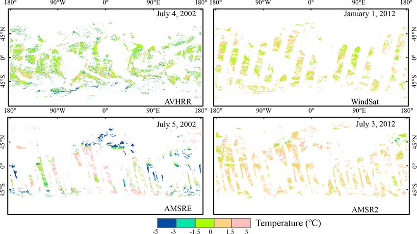
2114                 M. Cao et al.: A new global gridded sea surface temperature data product based on multisource data

   The AVHRR sensor is on board NOAA polar-orbiting                of both the satellite-obtained SST data and the new prod-
satellites, has six bands ranging in wavelength from visible to    uct. The SST data observed in situ used in this study con-
infrared (one visible, two near-infrared, and three thermal in-    sist of SSTs from the Version 2.1 NOAA in situ Quality
frared) and can cover the globe twice a day. The twice-daily       Monitor (iQuam), which includes updated observations ev-
(day and night) AVHRR 4 km SST data product is produced            ery 12 h with a 2 h latency. The SST data from iQuam include
by the NOAA National Centers for Environmental Informa-            observations from drifters, ships, tropical (T-) and coastal
tion and is available through the website https://data.nodc.       (C-) moorings, Argo floats, high-resolution (HR) drifters,
noaa.gov/pathfinder/Version5.3/L3C/ (last access: 6 Febru-         IMOS ships, and coral reef water (CRW) buoys, and the data
ary 2020). The standard deviation obtained in a data compari-      can be obtained from ftp://ftp.star.nesdis.noaa.gov/pub/sod/
son is approximately 0.68 ◦ C, as determined by a comparison       sst/iquam/v2.10/ (last access: 21 January 2020). Quality con-
of the AVHRR products with coincident ferry observations           trol of the data, including basic screening, duplicate removal,
(Barton and Pearce, 2006). The data also provided a qual-          plausibility, platform tracks, referencing, and cross-platform
ity index for each pixel based on the evaluation test results      and SST spike checks, was performed by the NOAA Cen-
stored in the pathfinder_quality_level metric, which allows        ter for Satellite Application and Research (Xu and Ignatov,
the identification of cloudy pixels and/or suspicious observa-     2014). Only SSTs assigned the best quality flag (i.e., level 5)
tions, with the quality level 0 representing the worst quality     were used in this study. To ensure the independence of the
and the quality level 7 being the best (Pisano et al., 2016). In   data reconstruction and the accuracy verification process, the
our data processing method, we only considered values with         data obtained from all spatially coincident in situ observa-
quality flags 4–7.                                                 tions of SST were randomly divided into two completely
   The AMSR-E sensor is on board the Aqua satellite and is         independent subsets by the jackknife method (Benali et al.,
a dual-polarization microwave scanning radiometer with six         2012). Subset 1 accounts for 80 % of the total number of in
frequency channels in the range of 6–89 GHz. The AMSR-E            situ observations, which were used to reconstruct the MODIS
instrument was in orbit for nearly 10 years but was discontin-     SST data. Subset 2 accounts for 20 % of the total number of
ued in October 2011, owing to an antenna rotation problem.         in situ observations, which were used to verify the accuracy
The AMSR2 sensor, on board the Global Change Observa-              of the reconstruction results. The spatially coincident crite-
tion Mission-Water 1 (GCOM-W1) satellite, was launched             rion restricts the maximum distance between in situ measure-
in May 2012 to continue the Aqua/AMSR-E observations               ments and the center of the satellite image grid cells to within
and ensure the continuity of SST data (Zabolotskikh et al.,        2.3 km, which is approximately half the spatial resolution of
2015). AMSR2 has the same channels as did AMSR-E, with             MODIS, so that the in situ observations always fall within
a 7.3 GHz channel added to help alleviate radio frequency          the MODIS SST pixels (Minnett, 1991; Pisano et al., 2016).
interference. However, SST information collected from the
AMSR2 sensor was not provided until mid-2012. To en-               2.3    Ancillary data
sure that there is an uninterrupted consistent long-term mi-
crowave SST time series that can be used to reconstruct a          ERA-Interim, a climate reanalysis product produced by
high-quality SST product, a WindSat polarimetric radiome-          the European Centre for Medium-Range Weather Forecasts
ter was used to bridge the gap between the AMSR-E and              (ECMWF), was discontinued on 31 August 2019 and has
AMSR2 products. The daily L3 SST products (ascending and           been superseded by the ERA5 reanalysis product produced
descending passes) of AMSR-E and AMSR2, available from             by the ECMWF. The ERA5 dataset is the latest climate re-
June 2002 and July 2012, respectively, with 0.1◦ -grid spatial     analysis product, providing hourly data on atmospheric, land,
resolutions, were used to reconstruct high-quality SST data        and oceanic climate parameters together with estimates of
and are available through the website https://gportal.jaxa.jp/     uncertainty. The 10 m wind component U , 10 m wind com-
gpr/search/ (last access: 9 February 2020). The accuracies of      ponent V , 2 m temperature, 2 m dew point temperature, sea
AMSR-E and AMSR2 are approximately 0.75 and 0.56 ◦ C,              surface temperature, relative humidity, cloud cover, and other
respectively, as determined by comparisons with buoy data          data from the two datasets with 0.25◦ spatial resolutions
(Sun et al., 2018). Daily WindSat SST datasets on a global         were used to calculate the heat, momentum, and fluxes be-
25 km grid (ascending and descending passes) were down-            tween the ocean and the atmosphere as well as the incom-
loaded online (http://www.remss.com/missions/windsat, last         ing solar radiation. These data can be obtained from https:
access: 16 February 2020), and their accuracies are very           //apps.ecmwf.int/datasets/ (last access: 15 January 2020).
close to that of AMSR-E, as determined by comparisons with
buoy data (Banzon and Reynolds, 2013; Gentemann, 2011).            3     Methodology

2.2    In situ observations
                                                                   Since MODIS SST data have a high accuracy and spatiotem-
                                                                   poral resolution which can be used to capture mesoscale phe-
In situ observations of SST from 2002–2019 were used for           nomena in the oceans, a combination of MODIS SSTs from
the reconstruction of the new SST product and the validation       Aqua and Terra is a good way to improve the spatial cover-

Earth Syst. Sci. Data, 13, 2111–2134, 2021                                         https://doi.org/10.5194/essd-13-2111-2021
M. Cao et al.: A new global gridded sea surface temperature data product based on multisource data                          2115

age of SST data. However, SSTs are retrieved using the ther-         The main source of the difference is the inconsistent wave-
mal infrared bands which are influenced much by clouds, so        length or frequency range used by different sensors, which
SST data cannot be provided when they have clouds in the          leads to the temperature information measured by the sen-
sky, and SST retrievals are also influenced by atmospheric        sors from different ocean depths. The thermal infrared re-
aerosols. Some other factors related to radiometers can also      mote sensor measures the sea surface skin temperature at
contaminate SST observations, such as the viewing geome-          a depth of 10–20 µm, while the microwave remote sensor
try, spectral response, and noise level of each sensor (Kil-      can retrieve the sea subcutaneous temperature at a depth
patrick et al., 2015). Due to these effects, MODIS SST data       of 1–1.5 mm (Minnett, 2003; Minnett et al., 2011). There-
often have problems involving low-quality or missing pix-         fore, the SSTs retrieved from various microwave radiome-
els. Statistical analysis performed during the study period in-   ters (AMSR-E, WindSat, and AMSR2) are different from the
dicated that the missing pixels present in the monthly SST        SSTs measured by the MODIS radiometer. In addition, due
records of Terra and Aqua during both daytime and nighttime       to the difference of the inversion algorithm parameters, the
generally cover 23.46 % and 28.06 % of the global ocean,          sea temperature retrieved from the same type of sensor may
respectively. In order to overcome these defects, we built        also be different. For example, although the AVHRR sen-
a reconstructed spatial model that combines in situ station-      sor is an infrared remote sensor and its brightness temper-
based data and daily SST data from AVHRR, AMSR-E,                 atures represent the sea surface skin temperature, AVHRR
AMSR2, and WindSat to generate a high-quality MODIS               SSTs correspond to subsurface SSTs because they are sta-
SST monthly dataset. Although the temperatures retrieved by       tistically regressed to coincident in situ buoy SSTs (Chao
different sensors are all ocean surface temperatures, they ac-    et al., 2009a; Kilpatrick et al., 2001; Pisano et al., 2016).
tually represent temperature information at different ocean       Starting with the AVHRR Pathfinder Version 5.3, an aver-
depths which are caused by different frequencies of different     age skin–subsurface temperature difference of 0.17 K, deter-
sensor settings and inconsistent algorithms. The sea tempera-     mined from Marine Atmospheric Emitted Radiance Interfer-
ture observed by thermal infrared is the skin temperature, and    ometer (M-AERI) matchups, was used to eliminate the sub-
the sea temperature observed by microwaves is a bit deeper        surface bias so that the SSTs were more closely tuned to
than the depth observed by thermal infrared. In addition,         the sea surface skin temperatures (Sea Surface Temperature-
the observation time of different observation methods may         Pathfinder C-ATBD). MODIS SSTs are skin SSTs. MODIS
be inconsistent. Therefore, we proposed a temperature depth       retrievals are based on empirical coefficients derived by re-
and observation time correction model to address the influ-       gressing MODIS brightness temperatures against in situ ob-
ence of time phase and sampling depth of different sensors.       servations from drifting and moored buoys, but the regressed
More details are given in the following sections. The overall     SSTs are converted to skin SSTs based on at-sea measure-
methodology is illustrated in Fig. 1. This processing effec-      ments. Thus, the SSTs retrieved from the AVHRR radiome-
tively retains the high-precision pixels in the original MODIS    ter are different from the SSTs measured by the MODIS
daily and monthly data, combines the calibrated ocean multi-      radiometer. In addition, MODIS and several other sensors
source data with spatiotemporal information to reconstruct        used in this paper have different observation times and can
the low-quality and missing daily pixels, and finally replaces    obtain measurements at several different times throughout
the low-quality and missing pixels in the monthly data.           the diurnal cycle. The relationships among these observa-
                                                                  tions are, however, not constant because there are signifi-
                                                                  cant diurnal variations in sea surface temperature resulting
3.1     Bias adjustment by constructing temperature depth         from constant changes in the atmosphere, solar heating, wind
        and observation time correction model                     speeds, etc. (Kilpatrick et al., 2015; Luo et al., 2019; Minnett
3.1.1    Bias adjustment scheme for multisource remote            et al., 2019; Wick et al., 2004). This also results in differ-
         sensing data                                             ences between MODIS observations and those of other sen-
                                                                  sors. Therefore, compensating for measurement depths and
To combine oceanic multisource remote sensing data into the       times is conducive to reducing the uncertainty present in the
MODIS SST product, it is necessary to assume that the mea-        reconstruction results before the multisource remote sensing
sured values represent the same quantities or to use some         data are combined into the MODIS SST product.
method to eliminate the differences among products. The
ocean temperature data obtained by different sensors are dif-      1. Compensating to ensure uniform effective sampling
ferent from those obtained by MODIS, and there are com-               depths.
plex spatiotemporal differences. Figures 2 and 3 represent             To solve the differences among MODIS and multi-
the difference distributions of the original MODIS and mul-            source daily SST products caused by the sampling
tisource daily SSTs in the daytime. Obviously, these multi-            depths, it is necessary to consider the differences as re-
source data cannot be directly used to reconstruct the valid           sults of the cool skin effect and diurnal heating (Luo
pixels of MODIS SST data before the differences are cor-               et al., 2020). The General Ocean Turbulence Model
rected.                                                                (GOTM) can model the SST signal at different depths

https://doi.org/10.5194/essd-13-2111-2021                                        Earth Syst. Sci. Data, 13, 2111–2134, 2021
2116                  M. Cao et al.: A new global gridded sea surface temperature data product based on multisource data

Figure 1. A summary flow chart for reconstructing MODIS monthly SST data.

                                                                        perature (Karagali et al., 2017; Pimentel et al., 2018).
                                                                        General ocean models typically simulate the surface
                                                                        layer of 5–10 m as a uniform layer, and simulating such
                                                                        thin sea surface skin layers and subskin layers takes a
                                                                        long time. The GOTM can use a non-uniform grid and
                                                                        specifically encrypt the surface layer to quickly simu-
                                                                        late the temperature of the sea surface skin layer and the
                                                                        subskin layer. For example, the top 50 m of the water
                                                                        column is resolved by using 50 vertical layers, which
                                                                        have higher resolution near the surface and gradually
                                                                        decrease with depth. The thickness of the first layer at
                                                                        the top of the water column is about 20 µm, and the
                                                                        thickness of each layer can be calculated according to
                                                                        Eq. (1).
                                                                                                k

Figure 2. Box chart with scatters of the differences in the original           tanh (dl + du ) M  − dl + tanh(dl )
                                                                        hk = D                                     − 1,            (1)
MODIS and multisource daily SSTs (AVHRR, WindSat, AMSR-                               tanh (dl ) + tanh(du )
E, AMSR2). The boxes are determined by the 25th and 75th per-
centiles. The whiskers are determined by the 5th and 95th per-          where hk represents the thickness of layer K. D repre-
centiles. The data are plotted as scatters on the left of each box.     sents the depth. M is the number of layers, and dl and
A curve corresponding to a normal distribution is also displayed on     du show the zooming factors of the surface and bottom,
top of each scatter plot.                                               respectively.
                                                                        From this formula, the following grids are constructed:

     by simulating the hydrodynamic and thermodynamic                       – dl = du = 0 results in equidistant discretization.
     processes of vertical mixing in one-dimensional water
                                                                            – dl > 0, du = 0 results in zooming near the bottom.
     columns in natural waters which has been successfully
     used to model the near-surface variability of ocean tem-               – dl = 0, du > 0 results in zooming near the surface.

Earth Syst. Sci. Data, 13, 2111–2134, 2021                                          https://doi.org/10.5194/essd-13-2111-2021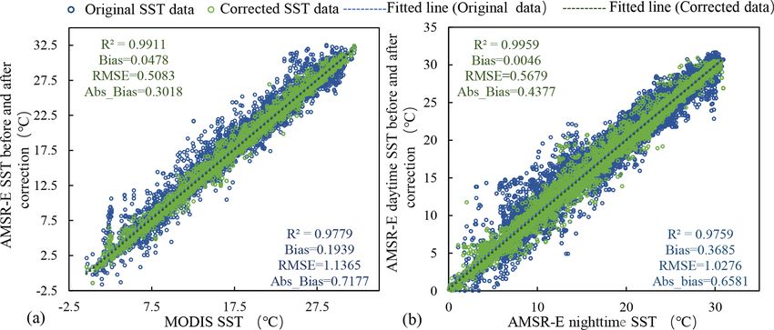
M. Cao et al.: A new global gridded sea surface temperature data product based on multisource data                            2117

Figure 3. Difference maps of the original MODIS and multisource daily SST products. Areas of missing data are blank.

       – dl > 0, du > 0 results in double zooming near both                conducted using the model by entering the SST mea-
         the surface and the bottom.                                       surement depth and the corresponding meteorological
                                                                           parameter values present during the measurement, in-
     Furthermore, considering the cool skin effect that usu-               cluding the wind speed at a 10 m height, the air tem-
     ally occurs in a molecular sublayer of the air–sea inter-             perature at a 2 m height above the sea surface, air hu-
     face, a physical model for the skin (as shown in Eqs. 2               midity data, and cloud cover data from the ECMWF.
     and 3) widely used to estimate the cold skin effect was               Figure 4a and b show the variations in ocean tempera-
     integrated into the air–sea interaction module of the                 tures at different depths and the differences between the
     GOTM (Fairall et al., 1996; Saunders, 1967). The heat                 sea surface skin temperatures and sea surface subskin
     and momentum flux changes of each layer in the water                  temperatures simulated by the GOTM every half hour
     column were integrated to more accurately simulate the                for a pixel with a longitude of 32.65◦ N and a latitude
     skin effects of the SSTs.                                             of 43.25◦ E from 1 July 2002 to 31 July 2002. When
                                                                           the wind speed is low, the infrared-measured SST is
     1T = Qδ/K,                                              (2)
                                                                           0.1–0.2◦ lower than that obtained by microwave remote
        λV                                                                 sensing. When the wind speed is high, the SSTs mea-
     δ=     ,                                                (3)
        µ∗w                                                                sured by the two sensor types are basically the same.
                                                                           By deducting this difference, the SSTs obtained by mi-
     where 1T is the temperature variation (positive, rep-
                                                                           crowave remote sensing can be normalized to the SSTs
     resenting that the surface is cooler than the bulk). Q
                                                                           obtained by infrared remote sensing.
     is the net heat flux. K is the thermal conductivity of
     water. δ is the thickness of the change in tempera-
                                                                        2. Compensating to ensure uniform measurement times.
     ture. λ is the empirical coefficient. V is the kinematic
     viscosity, and µ∗w is the friction velocity in the wa-                To solve the differences among the MODIS and multi-
     ter. It is difficult to obtain λ in Eq. (2). Based on                 source daily SST products caused by the varying mea-
     the observed data of the Tropical Ocean-Global Atmo-                  surement times, it is necessary to consider the diurnal
     sphere Coupled Ocean–Atmosphere Response Exper-                       variations in SST. The GOTM is based on the hydrody-
     iment (COARE) program, Fairall et al. (1996) deter-                   namic and thermodynamic processes of water and com-
     mined λ to be dependent on wind speed.In this section,                prehensively considers the effects of solar shortwave ra-
     the conversion of SSTs between different depths can be                diation, longwave radiation, latent heat, sensible heat,

https://doi.org/10.5194/essd-13-2111-2021                                            Earth Syst. Sci. Data, 13, 2111–2134, 2021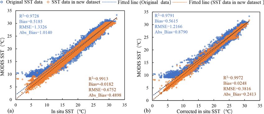
2118 M. Cao et al.: A new global gridded sea surface temperature data product based on multisource data
and cloudiness on diurnal variations in SST. The diurnal diurnal change corrections, the different measurement
variations caused by differences in the absorption and times and effective sampling depths were corrected.
attenuation of solar radiation of different water types However, the performances of different sensors are dif-
are also considered. Therefore, the GOTM can accu- ferent, and there may be systematic and regional devia-
rately simulate diurnal variations in SST. The input data tions, which need to be eliminated before fusion (Aler-
also come from the ECMWF reanalysis product and in- skans et al., 2020; Huang et al., 2015). Therefore, to cor-
clude the wind speed at a 10 m height, the air tempera- rect the large-scale deviations among different sensors,
ture at a 2 m height above the sea surface, air humidity we used the daily MODIS SST data to correct the other
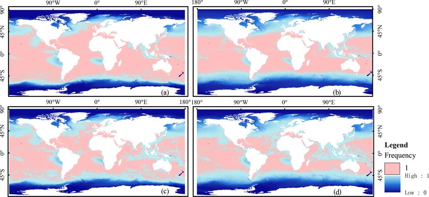
data, and cloud cover data. Cloudiness is used to cal- remotely sensed data compensating for different mea-
culate oceanic radiant heating. Wind speed, air temper- surement times and effective sample depths. Figure 5
ature, and relative humidity are used as inputs in the shows that the correlation coefficient of the MODIS
turbulence model to estimate sensible heat, latent heat, SST data and the other remotely sensed data reaches
and wind stress. The exchange coefficient of the turbu- above 0.97, indicating that these data have a strong cor-
lence equation is obtained based on the Fairall param- relation with the MODIS data. Therefore, we adopt a
eter method. Figure 4a shows the variations in ocean linear regression to modify the other remotely sensed
temperature at different half-hour increments for a pixel SST data. The correction method uses linear regression
with a longitude of 32.65◦ and a latitude of 43.25◦ from of two corresponding images, and the regression coeffi-
1 July 2002 to 31 July 2002. For the SSTs obtained at cient is determined by matching the data of the MODIS
different times, after deducting the diurnal variations in sensor and the other remotely sensed data. To avoid the
temperature simulated by the GOTM, the observations influence of individual outliers, points with standard de-
can be referenced to common time. The formula is as viations over 1 ◦ C or with a difference greater than 2 ◦ C
follows. from the corresponding MODIS datum in the matching
N
P window did not participate in the regression.
(SSTs (i) + (SSTg (j ) − SSTg (i)))
i=1
SSTs = , (4)
N 3.1.2 Bias adjustment scheme for in situ observations
where SSTs is the SST observed by the satellite. j is the SSTs retrieved from MODIS sensors are skin SSTs. How-
referenced common time. i is the effective observation ever, in situ SSTs from Version 2.1 NOAA iQuam are subsur-
of other moments by the sensor on the same day other face SSTs. For Argo floats, only the shallowest high-quality
than moment j , of which there are a total of N , and measurement is extracted and saved from each profile into
SSTg is the SST simulated by the GOTM, which also the iQuam dataset (the same algorithms are used for other
corresponds to moments i and j . in situ platforms, such as those on ships, drifters, and moor-
3. Bias adjustments of different sensor products. ings), along with its measurement depth. The closest mea-
surement to the surface of the Argo float is at a depth of 3–
In order to ensure that the corrections of depth and
8 dbar (0.15–0.2 m for drifters and ∼ 1 m for moorings). The
time are effective for each pixel, we calculated the dif-
differences between skin and subsurface SSTs, as described
ference range of high-quality pixels for different SST
by Donlon et al. (2002), can be as large as 1.0–2.0 ◦ C when
data. Then, we manually checked the correction results
the solar insolation is strong and the wind speed is weak. Fig-
of each invalid pixel, and we determined the outliers
ure 6 shows that the differences between the MODIS data and
according to the statistical difference range and other
the eight types of in situ SSTs from iQuam can be significant
satellite SST data. Finally, these outliers were adjusted
under different weather conditions. When combining in situ
based on mathematical statistics. For example, to deter-
SSTs into the MODIS SST product, such differences need
mine the temperature difference (1t) between the skin
to be accounted for. Therefore, in situ SSTs were first col-
surface temperature and sub-skin surface temperature of
located and made coincident with MODIS data (within ±1 h
the pixel i of the MODIS data, we first calculated the
and ±0.02◦ of latitude and longitude). Then, the coincident
high-quality value of a pixel of MODIS data and the
in situ SSTs were adjusted using the temperature depth and
microwave data at the corresponding time during the
observation time correction model by entering the SST mea-
study period. Then we extracted the data of wind speed,
surement depth and corresponding meteorological parameter
cloud cover, humidity, and other environmental factors
values present during the measurement, including the wind
corresponding to these values. Further, based on these
speed at a 10 m height, the air temperature at a 2 m height
environmental factors, we determined the SSTs corre-
above the sea surface, air humidity data, and cloud cover data
sponding to the environmental conditions at the moment
from the ECMWF.
when the outlier of pixel i appeared. Lastly, the aver-
age value of the differences between these high-quality
SSTs was 1t. After completion of the above depth and
Earth Syst. Sci. Data, 13, 2111–2134, 2021 https://doi.org/10.5194/essd-13-2111-2021
M. Cao et al.: A new global gridded sea surface temperature data product based on multisource data                                       2119

Figure 4. SST depth changes simulated by the GOTM every half hour for a pixel with a longitude of 32.65◦ and a latitude of 43.25◦ in
July 2002 (panel a is the variation in ocean temperature at different depths; panel b is the difference between the sea surface skin temperature
and sea surface subskin temperature).

Figure 5. Scatter diagrams of the MODIS SST data and ocean multisource data compensated for different measurement times and effective
sampling depths.

3.2   Filtering of MODIS SST                                              are mainly distributed in high-latitude sea areas beyond ±60◦
                                                                          of latitude. In the middle- and low-latitude sea areas within
The monthly MODIS SST data cover the whole sea area of                    ±60◦ of latitude, the coverage rate of pixels is more than
the world, but they contain many missing and low-quality                  95 %. There are many missing pixels distributed off the Peru
pixels caused by factors such as clouds and aerosols. Fig-                coast, in the El Niño–Southern Oscillation (ENSO) signal re-
ure 7 shows the frequency of non-null pixels, including valid             gion, due to the widespread low clouds over the eastern South
pixels and low-quality pixels, in the monthly MODIS SST                   Pacific off the coasts of Chile and Peru (Satyamurty and
data from July 2002 to December 2019. The missing pixels                  Rosa, 2020). In addition, there is a lower frequency of non-

https://doi.org/10.5194/essd-13-2111-2021                                                  Earth Syst. Sci. Data, 13, 2111–2134, 2021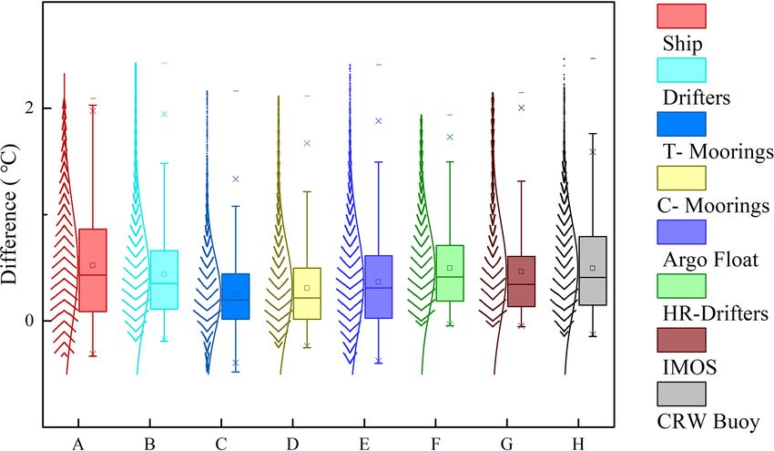
2120                  M. Cao et al.: A new global gridded sea surface temperature data product based on multisource data

                                                                     (i.e., the low-quality and missing pixels) in the monthly im-
                                                                     ages, we filtered the daily MODIS SST data of the respective
                                                                     month at the corresponding location. The high-quality pix-
                                                                     els in the daily SST data were retained, and the invalid pix-
                                                                     els in the daily data were reconstructed by combining multi-
                                                                     source data. Finally, the invalid pixels present in the monthly
                                                                     data were replaced by the mean SST values derived from the
                                                                     gap-filled daily SST time series of the corresponding month.
                                                                     Combining the characteristics of multisource data and the
                                                                     availability of the data, we adopted different methods to re-
                                                                     construct the invalid pixels present in the daily MODIS SST
                                                                     data for different regions.
Figure 6. Box chart with scatters representing the differences be-
tween the original MODIS data and eight types of in situ SST ob-     3.3.1   Reconstruction of invalid SST pixels in low-latitude
servations.                                                                  and midlatitude marginal regions of the ocean
                                                                     Due to the influence of the mixed pixels in adjacent coastal
null pixels in the Inter-Tropical Convergence Zone (ITCZ)            areas, sea surface temperature products obtained from pas-
region and other tropical oceanic areas west of the continents       sive microwave remote sensing have very large uncertainties
due to the cloud cover in these areas (Ackerman et al., 2008;        in these areas (Xie et al., 2008), which result in more invalid
McCoy et al., 2017). In most areas of low and middle lati-           or low-quality pixel values in adjacent coastal areas. There-
tudes, the non-null pixel coverage is as high as 100 %, but          fore, invalid pixels in these regions were first filled with in
it is difficult to detect the cold top surface of thin clouds or     situ or AVHRR SST data, and these pixels filled with in situ
subpixel clouds, and the SSTs retrieved under such condi-            observations were marked. Then, in cases where these obser-
tions are usually underestimated because the temperatures of         vations were missing, we filled these invalid pixels based on
clouds are almost always colder than the temperature of the          the geographically weighted regression (GWR) and Kalman
sea surface (Reynolds et al., 2007). Moreover, other factors         filtering (KF) methods, fitted the SSTs obtained by the two
can also contaminate the observed signals and affect the data        methods, and finally reconstructed the invalid pixels. A sum-
quality, such as factors related to the radiometer, including        mary flow chart of the process is schematically illustrated in
its viewing geometry, spectral response, and noise level (Kil-       Fig. 8.
patrick et al., 2015). Therefore, there are many low-quality
pixels among non-null pixels in the low and middle latitudes          1. Interpolating invalid pixels with GWR.
during the study period. In this study, the spatial process of            GWR is an effective method for estimating missing pix-
the SST reconstruction includes the removal of low-quality                els, which can quantitatively determine the contribution
pixels in low-latitude and midlatitude regions and the recon-             of adjacent pixels to contaminated pixels (Zhao et al.,
struction of low-quality and missing pixels in the low-latitude           2020). This method assumes that the spatially adjacent
and midlatitude regions and the high-latitude regions.                    pixels with similar meteorological conditions have sim-
   The quality control information stored in the qual_sst layer           ilar temperature values. Therefore, after determining the
is provided along with the MODIS L3m SST data, with the                   pixels, the GWR method was used to reconstruct invalid
quality level 0 being the best quality and the quality level 4            pixels. To determine the sliding window with the min-
being the worst. These values can be found in the original                imum noise and the best complement value, we simu-
MODIS SST netCDF files (see Sect. 2.1 for a detailed de-                  lated the size of the experimental pixel window many
scription). The missing pixels present in these data are rep-             times and selected a sliding window of 15 by 15 pix-
resented by the filling value −32 767. Therefore, the quality             els centered on the target pixel. This window size also
control labels and the filling value were used to identify low-           avoids the reduction in execution efficiency caused by
quality and missing pixels in the MODIS SST product. For                  the redundancy of pixel involved in the calculation and
monthly and daily SST data, to ensure the data quality and                ensures the number of pixel values involved in the cal-
the number of effective pixels, pixels with a quality level ≤ 1           culation. During the reconstruction of invalid pixels,
were considered to be high-quality data.                                  the regression weight coefficient of each adjacent pixel
                                                                          was determined by the Euclidean distance between that
3.3    SST data reconstruction
                                                                          pixel and the target pixel. Simultaneously, considering
                                                                          that the available pixels obtained from in situ observa-
In the data processing, we first filtered all input monthly               tions are more representative of the real SST under the
MODIS SST images and determined the locations of the                      cloud cover, we assigned a relative multiple weight to
low-quality and missing pixels. Then, for each invalid pixel              the marked in situ data according to GWR. By select-

Earth Syst. Sci. Data, 13, 2111–2134, 2021                                           https://doi.org/10.5194/essd-13-2111-2021
M. Cao et al.: A new global gridded sea surface temperature data product based on multisource data 2121
Figure 7. Frequency of non-null pixels, including valid pixels and low-quality pixels, in the monthly MODIS SST data during the study
period from (a) nighttime Aqua overpasses, (b) daytime Aqua overpasses, (c) nighttime Terra overpasses, and (d) daytime Terra overpasses.
Mc
Di
Wi = P Mg
m Mc Pn
i=1 Di + j =1 Dj
Mg
Dj
Wj = P Pn Mg (6)
m Mc
i=1 Di + j =1 Dj
Xm Xn
Tt = i=1
W i · T i + W
j =m+1 j
· Tj (7)
Here D is the distance from the adjacent pixel to the tar-
get pixel. (x, y) and (xt , yt ) are the locations of the adja-
cent pixel and target pixel, respectively. i and j are the
adjacent pixels used to estimate the SST of the invalid
pixel. i is an adjacent pixel of high quality. j is a pixel
assigned by in situ measurement. Wi and Wj are weight
multipliers. m is the number of i. n is the number of j ,
Figure 8. A summary flow chart for reconstructing invalid SST pix- and Mc and Mg represent the weighting coefficients of
els in low-latitude and midlatitude marginal regions of the ocean. the high-quality pixels and in situ assignment pixels, re-
spectively. Mc and Mg are set at 1 and 3, respectively.
Tt is the filled SST value of the target pixel.
ing some marked pixels as experimental values, it was 2. Using KF to coordinate the error.
found that the target pixels can be estimated accurately
when Mg (Mg is the weighting coefficient of the in situ For this region, on the basis of interpolation, KF can
assigned pixels) was set to 3. The weighting coefficients be used to coordinate the error characteristics of the
of adjacent pixels can be determined by Eqs. (5) and SST variation and the error characteristics of the in-
(6). Then a local linear regression calculation was per- terpolation. Since the SST variation is relatively flat,
formed for each point in the window according to the SST is treated as a stationary random process. Due to
sample weights. This regression calculation can be ex- the slowly changing characteristics of SST and the lack
pressed as Eq. (7). of effective temperature values representing these pix-
els, we took into account the SST data representing the
q adjacent time at the location of the invalid pixel. Con-
D= (x − xt )2 + (y − yt )2 (5) sidering the operational requirements of SST real-time
https://doi.org/10.5194/essd-13-2111-2021 Earth Syst. Sci. Data, 13, 2111–2134, 20212122 M. Cao et al.: A new global gridded sea surface temperature data product based on multisource data
retrievals and the necessary computing speed and stor- 3. Fitting interpolated and filtered data.
age capacity of the computer, the correlation of the error To more accurately reconstruct the pixels that lack valid
changes with each observation time was not considered observations, a data fitting shown in Eq. (15) was per-
in the actual operation process, and only the simple ran- formed for the interpolated and filtered data, which are
dom error was used to simulate the changes in the pro- the SSTs obtained based on the GWR and the KF meth-
cess error and measurement error. By modeling the data, ods, respectively. Finally, the reconstruction of invalid
the equation of the state of the system can be written as pixels without in situ or AVHRR SST filling could be
follows. realized by using the data fitting.
X t = ∅X t−1 + W t−1 , (8)
T 0 = αTg + βTk , (15)
where Xt is state to be estimated at time instant t. Xt−1
is the state vector of the process at time t. ∅ is the state where T 0 is the reconstructed SST. Tg and Tk are the
transition matrix of the process from the state at t − 1 to SSTs obtained based on the GWR and the KF methods,
the state at t, which is assumed stationary over time, and respectively.
W t−1 represents the process noise, which is considered To determine the best fitting parameters of α and β, we
to be Gaussian, and its covariance is represented by Q. selected some valid pixels from each image and then
We take the KF of 124 MODIS SST images in July 2002 interpolated and filtered these pixels. The Eq. (15) was
as an example. All data were arranged in chronological used to fit the interpolated and filtered results, and the
order, and the change of the SST in each pixel relative fitting coefficients of each SST image were obtained us-
to the SST of the previous time was counted. Based on ing the least-squares method.
the statistical results of these images, the covariance was n
X
3.115·I (I is the identity matrix). Consider the following 1T (α, β) = [Ti − Ti0 ]2 , (16)
measurement equation. i=1
Z t = HXt + V t , (9) where Ti is the valid pixel value in the image and n is the
number of these pixels. When 1T reaches a minimum
where Z t is the measurement of X at time instant t.
value, the fitting coefficient can be obtained by using
H is the noiseless connection between the state vector
Eqs. (17) and (18).
and the measurement vector, which is assumed station-
ary over time. V t represents the measurement noise, n
∂1T (α, β) X
which is also considered to be Gaussian, and its covari- = −2 Ti − αTg − βTk Tg = 0 (17)
∂α i=1
ance is represented by R. R can be obtained by compar-
n
ing the measurement data with the verification data (Xu ∂1T (α, β) X
= −2 Ti − αTg − βTk Tk = 0 (18)
and Cheng, 2021). Then, the following KF formula was ∂β i=1
used to combine the input data to achieve the optimal
output of the system, which operates in a prediction up-
3.3.2 Reconstruction of invalid SST pixels in low-latitude
date. The prediction equations are responsible for pro-
and midlatitude inner ocean areas
jecting forward (in time) the current state and error co-
variance estimates to obtain the a priori estimates for the Similar to the method used to reconstruct invalid SST pix-
next time step. The update equations are responsible for els in the marginal regions of the oceans at low and middle
the feedback, i.e., for incorporating a new measurement latitudes, pixels with invalid SST values were reconstructed
into the a priori estimate to obtain an improved a poste- through collocating with in situ and AVHRR data in inner
riori estimate. Prediction equations are as Eqs. (10) and ocean areas. The invalid pixels were filled using values from
(11). valid in situ SST or AVHRR data collected at the same lo-
cation at the same time. In cases of missing in situ SST or
X−
t = ∅X t−1 (10)
AVHRR data, the SST was retrieved from passive microwave
T
P−
t = ∅Pt−1 ∅ + Q (11) data to reconstruct the invalid SST data. A summary flow
chart of the process is schematically illustrated in Fig. 9.
Update equations are as Eqs. (12), (13), and (14).
The temperature variation trends present in the MODIS
T − T
Kt = P−
t H [HPt H + R]
−1
(12) daily data and microwave daily data on corresponding date
Xt = X− − in the same region are the same, so the two groups of data
t + Kt [Zt − HX t ] (13)
have the same proportional relation. Taking a grid of n pixels
Pt = [I − Kt H]P−t (14)
by n pixels as an example, a and b are considered the same
Here X, ∅, H, Q, and R can be obtained according to regions clipped from the MODIS and microwave-based data,
the explanation of Eqs. (8) and (9). K is the Kalman respectively. The gray and white rasters represent the effec-
gain. P is the error covariance matrix. tive and invalid pixels, respectively. Mkl and Rkl represent
Earth Syst. Sci. Data, 13, 2111–2134, 2021 https://doi.org/10.5194/essd-13-2111-2021M. Cao et al.: A new global gridded sea surface temperature data product based on multisource data 2123
number of field observations at the area is generally scarce
compared to other regions (Reynolds et al., 2002). The Mi-
crowave and AVHRR SST data used in this study have lim-
ited available pixels in high-latitude regions, so it is impossi-
ble to reconstruct MODIS SST data in high-latitude regions
only by relying on these data and in situ data.
High-latitude SSTs can be estimated based on satellite sea
ice concentrations (SICs). In areas with sea ice, the SST
is the temperature of the open water or of the water under
the ice (Banzon et al., 2020). Multiple analysis (L4) prod-
ucts from GHRSST enable SST estimation near the polar re-
gion by converting SIC into SST. Due to differences in satel-
lite source data, integration methods and methods for con-
verting SIC to SST, the accuracy of level-4 SST products
Figure 9. The summary flow chart for reconstructing invalid SST of GHRSST-PP varies in many aspects. After understanding
pixels in low-latitude and midlatitude inner ocean areas. the differences among current GHRSST level-4 products and
their qualities and availabilities in different areas, the OISST
V2.1 product was selected to restore invalid pixels in the
the pixel values of the MODIS and microwave-based data,
MODIS SST data in the high-latitude area with sea ice cov-
respectively. K and L represent the pixel positions. Mij rep-
erage. In the product, SICs were revised to SSTs to remove
resents the value after the interpolation of invalid pixels.
warm biases in the Arctic region.
Mij In areas of high latitudes, since the microwave-based SST
k=i−1,l=j
P −1 k=n,j
P=n data (used in this paper) exclude sea ice pixels, that is, SSTs
Mk,l + Mk,l are missing when the number of pixels with sea ice contam-
k=1,l=1 k=i+1,l=j +1 ination exceeds a specified value, we used a combination of
Rij two strategies to reconstruct the missing SST data to improve
= (19)
k=i−1,l=j
P −1 k=n,j
P=n the accuracy of the results. A summary flow chart of the pro-
Rk,l + Rk,l cess is schematically illustrated in Fig. 11.
k=1,l=1 k=i+1,l=j +1
First, the variables l2p_ flags and the sea ice fraction in
The reconstruction of invalid pixels can be achieved by using the AVHRR SST data were used to identify the sea ice ex-
the above formula. The reconstructed pixels meet the accu- tent. The sea ice fraction variable quantified the fraction of
racy of the interpolated images to a certain extent and do sea ice contamination in a given pixel (ranging from 0 to 1),
not damage the original SST variation trend. After several and bit 2 of the l2p_ flags variable was recorded if an in-
simulations of different experimental pixel window sizes, the put pixel recorded ice contamination. These variables can be
noise was found to be minimized when a sliding window of used to identify sea ice pixels. Then, we used the first strat-
6 by 6 pixels was used, and this window size was considered egy to reconstruct invalid pixels in high latitudes without sea
to have the best complement value. ice coverage. Pixels with invalid SST values in the MODIS
data were collocated with in situ and AVHRR observations.
Invalid pixels were filled using the values from the valid in
3.3.3 Reconstruction of invalid SST pixels in
situ or AVHRR data at the same location and the same time
high-latitude regions of the ocean
(priority was given to the use of in situ data). Then, for the
At high latitudes, sea ice covers a significant fraction of invalid pixels without available observations, we used the
the global oceans (approximately 5 %–8 %). The presence of method described in Sect. 3.3.2 above to fill the pixels us-
large areas of mixed sea ice and open water makes it difficult ing microwave data. Finally, considering the characteristics
to retrieve SSTs (Høyer et al., 2012; Vincent et al., 2008). In of the slow changes in SST and the fact that SST changes
addition, there is persistent cloud cover in polar regions, with in the same area are interannual and its changes in the short
cloud cover occurring up to 90 % of the time in summer and term are usually small, the invalid pixels without any filling
50 %–60 % of the time in winter in the Arctic (Høyer et al., data were reconstructed by using the GWR method combined
2012). The continuous cloud cover and extended twilight pe- with spatiotemporal information. That is, we replace invalid
riod complicate the detection of cloud, which thus presents pixels with the average value of valid pixels from the adjacent
problems for identifying clouds correctly with cloud detec- dates. If the number of effective pixels was too small, then the
tion algorithms. Therefore, it is challenging to use satellite GWR method was used to reconstruct the invalid pixel. In
sensors to accurately retrieve SST at high latitudes, includ- another strategy, pixels with invalid SST values due to sea-
ing the Arctic Ocean. Moreover, because of the existence of ice-covered areas were collocated with in situ and AVHRR
sea ice and the difficulty of navigating in ice-filled water, the SSTs, which were filled using values from valid in situ SST
https://doi.org/10.5194/essd-13-2111-2021 Earth Syst. Sci. Data, 13, 2111–2134, 2021You can also read