A novel diagnostic method based on filter bank theory for fast and accurate detection of thermoacoustic instability - Nature
←
→
Page content transcription
If your browser does not render page correctly, please read the page content below
www.nature.com/scientificreports
OPEN A novel diagnostic method
based on filter bank theory
for fast and accurate detection
of thermoacoustic instability
Seongpil Joo1,5, Jongwun Choi2,5, Namkeun Kim2* & Min Chul Lee3,4*
This study proposes and analyzes a novel methodology that can effectively detect multi-mode
combustion instability (CI) in a gas turbine combustor. The experiment is conducted in a model gas
turbine combustor, and dynamic pressure (DP) and flame images are examined during the transition
from stable to unstable flame, which is driven by changing fuel compositions. As a powerful technique
for early detection of CI in multi-mode as well as in single mode, a new filter bank (FB) method based
on spectral analysis of DP is proposed. Sequential processing using a triangular filter with Mel-scaling
and a Hamming window is applied to increase the accuracy of the FB method, and the instability
criterion is determined by calculating the magnitude of FB components. The performance of the
FB method is compared with that of two conventional methods that are based on the root-mean-
squared DP and temporal kurtosis. From the results, the FB method shows comparable performance
in detection speed, sensitivity, and accuracy with other parameters. In addition, the FB components
enable the analysis of various frequencies and multi-mode frequencies. Therefore, the FB method can
be considered as an additional prognosis tool to determine the multi-mode CI in a monitoring system
for gas turbine combustors.
Recently, most gas turbines have adapted a premixed combustion that can reduce hazardous emissions, such
as NOx and unburned hydrocarbons, by decreasing the flame temperature and enhancing the mixing of air
and fuel1–3. However, this has a high risk of combustion instability (CI) caused by: (1) the lower sustainability
of flame anchoring; and (2) the higher probability of coupling between pressure fluctuation and heat release
fluctuation in both time and p osition4–6. CIs are a physical phenomenon that occur in reacting flows (e.g., a
flame) due to constructive coupling processes between acoustic pressure fluctuations and heat release oscilla-
tions in the combustion zone. The CI generally accompanies strong pressure vibration to cause damage to the
components of the combustor. Furthermore, the debris detached from the combustor can lead to fatal failures
of the downstream parts, such as turbine blades and vanes. Thus, CI has been investigated for more than three
decades, both theoretically7–9 and e xperimentally10–15, to understand its mechanism and devise methods of
diagnosis and control.
In view of practical applications of the combustion monitoring of real engines, several diagnostic tools have
been introduced to rapidly and accurately detect the onset of CI before it evolves to a significant level16–23. Table 1
summarizes representative parameters or analysis methods utilized for CI diagnosis.
The growth or damping rate ( ν ) is a parameter that quantifies the acoustic driving/damping capacity
in a system comprised of an injector and a c hamber24–27. It similarly works as a damping coefficient of the
mass–damper–spring system; thus, if ν > 0, the driving contribution of the acoustic–flame interaction overcomes
the dissipation of acoustic energy, and the system remains unstable. On the other hand, if ν < 0, the driving of
the acoustic–flame interaction is less than the dissipation of acoustic energy, so that the system remains stable.
Thus, this parameter has been used when expressing the trend of development or decay of CI. In particular, Yi
et al.26 investigated a damping ratio for the pressure spectrum using a weighted least mean squares (LMS) algo-
rithm, and they successfully showed that the damping ratio drops rapidly when a nonlinear limit cycle oscillation
1
Gas Turbine Laboratory, National Research Council of Canada, Ottawa, ON, Canada. 2Department of Mechanical
Engineering, Incheon National University, Incheon 22012, Republic of Korea. 3Department of Safety Engineering,
Incheon National University, Incheon 22012, Republic of Korea. 4Research Institute of Engineering and Technology,
Incheon National University, Incheon 22012, Republic of Korea. 5These authors contributed equally: Seongpil Joo
and Jongwun Choi. *email: nkim@inu.ac.kr; LMC@inu.ac.kr
Scientific Reports | (2021) 11:3043 | https://doi.org/10.1038/s41598-020-80427-6 1
Vol.:(0123456789)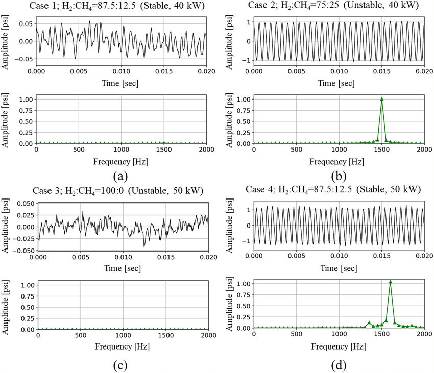
www.nature.com/scientificreports/
Parameter or method Description References
Growth/damping rate ( ν) is a parameter which quantifies the acoustic-driving/damping capacity in the system of an injector
and a chamber so it expresses the tendency toward to amplification/dissipation of combustion instability. It similarly works as a 24–27
Growth or damping rate
damping coefficient of mass-damper-spring system. If ν > 0, meaning that the driving contribution of the acoustic-flame inter-
action overcomes the dissipation of acoustic energy and the system stay as unstable. However, if ν < 0, system is stable status
Phase portraits are tools to analyze the nonlinear dynamics of a given signal by expressing all states of the physical system in 28, 29
Phase portraits and recurrence plot
phase space and the recurrence plot is a parameter that visualizes the recurrence of phase space trajectories
The complex networks are derived from the time-series dynamic pressure data that represents the system dynamics using the
visibility algorithm. The use of complex network helps to formulate the pattern emerging during the transition in combustion 18, 30
Complex network analysis
dynamics. Especially, a method combining turbulence network that each fluid element is connected via vortical interaction and
machine learning18. It can detect a small change in the combustion transition process
Temporal RMS is a representative value for describing a characteristic or trends of a dynamic pressure signal. When a signal
31–34
Temporal root mean square changes in magnitude and sign over time, RMS can indicate the only average magnitude of squared value of the dynamic pres-
sure signal
Temporal kurtosis is a time-domain statistical parameter, which contains the statistical distribution-quantity of “peakedness” 14, 35, 36
Temporal kurtosis
and “tailedness”
Table 1. Various parameters or analysis methods for evaluating combustion status.
Frequency [Hz] Expected level [psi, pk-pk] Maximum acceptable level [psi, pk-pk] Impact
100–135 < 0.5 1 Hardware damage
140–180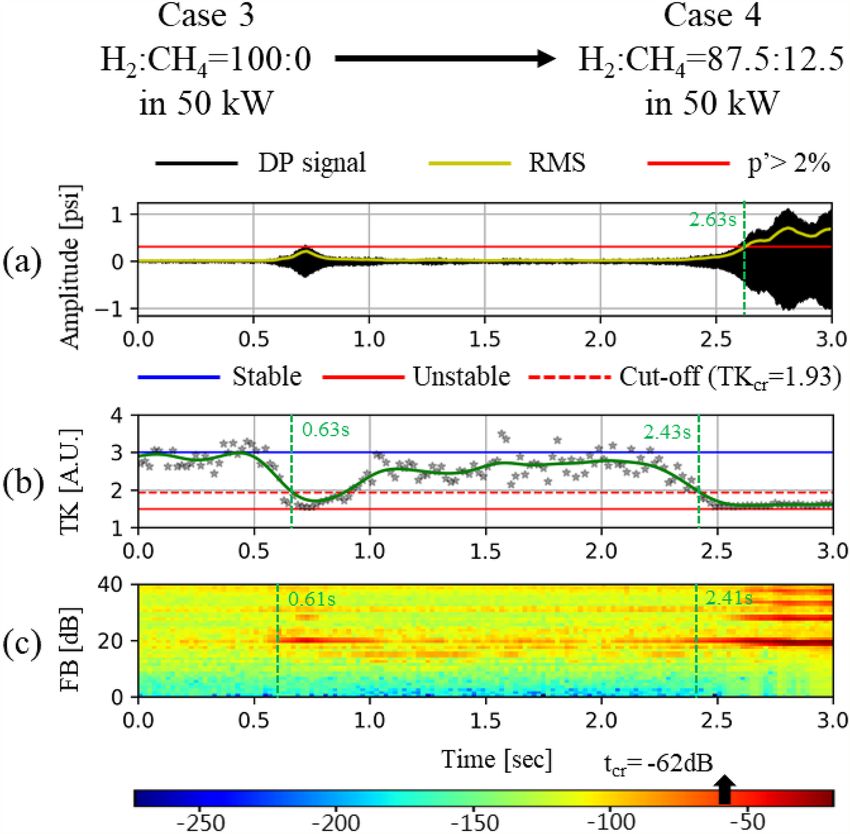
www.nature.com/scientificreports/
Figure 1. Schematic of the model gas turbine combustor and an enlarged view of the combustor head in
Region.
of H2/CO/CH4 synthetic gases50, which is definitely differentiated from the single-mode phenomenon occurring
during combustion of natural gas or methane.
The performance of the FB method is validated by comparing the accuracy and speed of detection with
those of three conventional methods: temporal root mean square (RMS), and temporal kurtosis (TK), for which
descriptions are listed in Table 1. Since the RMS is the most standard method of CI diagnostics and is widely
applied to commercial engines, RMS is firstly selected as a comparison t ool31–34. TK is chosen secondly, because
it is one of the recent methods that can judge the onset of CI, based not on the magnitude of DP but on the
periodicity14, 35, 36. That is, since the TK contains information on the statistical quantity of “peakedness” and
“tailedness,” the distribution and shape of DP can be used when determining the CI driving or decaying. There
are other approaches similar to TK. For example, entropy of energy36 and permutation entropy51, 52 are recent
approaches for CI diagnostics based on the signal distribution. In these methods, TK is widely used in the
acoustics and CI detection; thus, it has also been selected as a parameter for comparison. From the comparisons
with these methods, the better performance of FBs is verified by providing detailed clues, such as advances in
sensitivity of CI detection, shorter calculation time with a simpler algorithm and, consequently, earlier and more
precise detection results.
Experimental and data processing methods
Model gas turbine combustor. To obtain experimental CI data, a model gas turbine combustor, which
generates partially premixed flames, was utilized. As shown in Fig. 1, the fuel mixture and air were supplied in
parallel in the coaxial direction through separate injecting holes. At the end of each hole, 14 swirl vanes oriented
at 45° with respect to the longitudinal axis of the combustor enabled the two different types of fluids to mix.
Despite having a very short mixing length (Lmixing = 2.7 mm), it had a strong swirl number; thus, mainly bluish
flames appeared similar to a premixed flame.
3
2 1 − Dswirl_in /Dswirl_out
Sn =
tan φ (1)
3 1 − Dswirl_in /Dswirl_out 2
where Dswirl_in and Dswirl_out are the inner and outer diameters of the swirl vane; and ф is the swirl vane angle.
From Eq. (1), the swirl number is calculated to be 0.8353.
This combustor mainly generates a longitudinal CI mode rather than a radial or tangential mode because
the combustor length from the dump plane to the plug nozzle ( Lc = 1440 mm) is relatively longer than the
Scientific Reports | (2021) 11:3043 | https://doi.org/10.1038/s41598-020-80427-6 3
Vol.:(0123456789)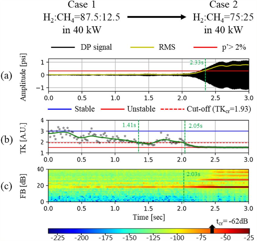
www.nature.com/scientificreports/
Parameter Value
Fuel H2, CH4
Air flow rate 1100 SLPM (0.18 kg/s),
Air temperature 200 °C (= 473 K)
Heat input (LHV) 40 kW, 50 kW
Equivalence ratio 0.55
H2 ratio [ H2 +CH
H2
H2 +CH4 ]
H2 0–100% (span of 12.5% by volumetric ratio)
4
Combustor length 1440 mm
Table 3. Experimental test conditions.
radius of the combustor. The dump plane and plug nozzle can be assumed to form acoustically-closed bound-
ary conditions.
n·c
f =
2·L
, n = 1, 2, 3, · · · , c = γ · R · Tc (2)
c
where γ is the adiabatic index; R is the gas constant; Lc is the combustor length; Tc is the mean temperature in the
combustor; and c is the speed of sound in the combustion zone. Using Eq. (2), the frequency of the fundamental
longitudinal mode is calculated to be 248 Hz54. As n changes in Eq. (2), the CI can have other higher modal
frequencies. Furthermore, several modes can occur simultaneously in a combustor.
High‑speed measurements for CI observation. To investigate the fast periodic fluctuation of CI, the
DP was measured at a rate of 16,000 Hz using a DP sensor (model 102A05, PCB Piezotronics, US) on the dump
plane closest to the flame. The DP data were recorded for 3.0 s, which was sufficient to investigate the transition
of the DP characteristics from the stable state to the unstable state.
An intensified charge-coupled device camera (model: PI-Max2; 1024 × 1024 pixels; Teledyne Princeton Instru-
ments, US) was also used to observe the flame variation with respect to the fuel composition. An OH bandpass
filter (307 ± 10 nm) was installed on the camera to obtain chemiluminescent signals of the OH radical. As the OH
chemiluminescent signals represented the heat release characteristics of the combustion zone, this information
was used to identify the structural characteristics of the flame.
Experimental conditions. Table 3 lists the experimental conditions. In this study, highly pure fuels of
hydrogen (H2) and methane ( CH4) (purity: H2 > 99.5 mol%, CH4 > 99.5 mol%) were used to ensure the reliability
of the experiment. The fuel and air flow rates were controlled by mass flow controllers (for air: model F-206BI,
Bronkhorst High-Tech, Netherlands; for fuel: Porter-200, Parker Hannifin Corp., US). The combustion air was
supplied at a flow rate of 1100 SLPM (0.02 kg/s) at a temperature of 200 ± 3 °C. The heat input was varied at
40 kW and 50 kW based on the lower heating value (LHV) of each fuel species. The equivalence ratio was fixed
at 0.55. The pressure in the combustor remained almost constant at 1.1–1.2 barg while the fuel compositions of
H2, CH4, and the heat inputs were changed to find the stable and unstable regions. Specifically, the H 2 ratio was
defined as the ratio of the volumetric flow rate of H
2 to the sum of those of H
2 and CH4. The H2 ratio was varied
from 0 to 100% with an increment of 12.5%.
Data processing method. Before introducing the details of the FB method for CI analysis, the TK method,
which will be compared with FB, is briefly reviewed.
Temporal kurtosis. In order to quantify the instantaneous “peakedness” and “tailedness” of the statistical distri-
bution of a given signal, the TK is calculated as follows:
− 4
1 n p
n i=1 pi −
TK =
2 (3)
− 2
1 n p
n i=1 pi −
where n is the number of−DP data values for a duration of given time (T); pi is the instantaneous DP signal at time
t = ti (i = 1, 2 …, n); and p is the mean DP. The TK has the theoretical value according to the given data proper-
ties. That is, whereas the TK for a random Gaussian distribution (i.e., a stable status in a combustion) is 3.0, the
TK for a sinusoidal signal (i.e., an unstable status in a combustion) is 1.5. In a practical combustor, however, the
DP signal of a stable status can be not a perfect Gaussian distribution, which means that the TK cannot be 3.0
in spite of the stable combustion status. To avoid this shortcoming, previous studies used the average value of
several TKs through a linear regression rather than the single TK value35. On the contrary, it should be noted
that the FB method suggested in the current study can assess the combustion status with only the single value
at a specific moment.
Scientific Reports | (2021) 11:3043 | https://doi.org/10.1038/s41598-020-80427-6 4
Vol:.(1234567890)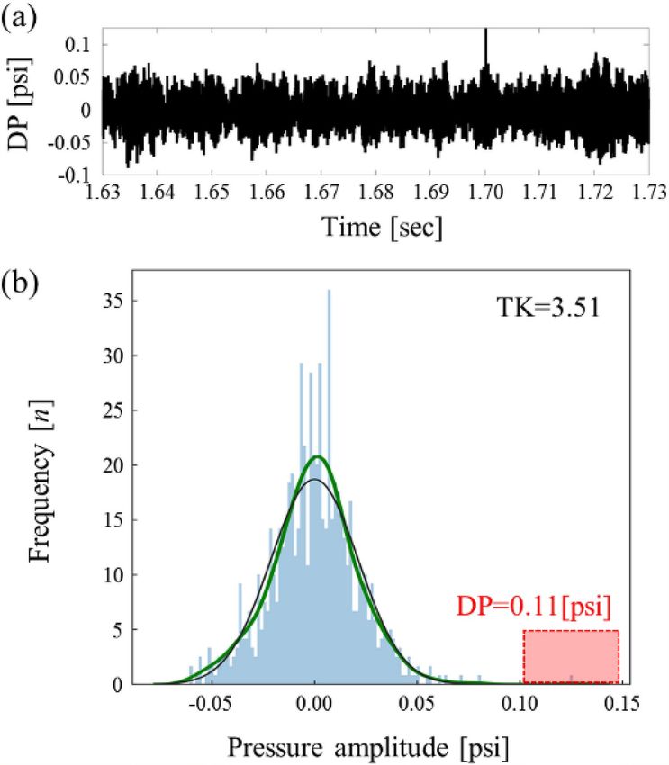
www.nature.com/scientificreports/

                                  Figure 2.  Flowchart of the FB processing method for CI diagnosis.

                                  Filter bank. The FB is a signal processing method based on an array of bandpass filters. It can detect the char-
                                  acteristics of various frequency bands by generating subband filters and multiplying them with the power spec-
                                  trum of each frequency obtained from a given dataset. In this study, the FB of DP signals was calculated and
                                  used as a CI precursor. As the first step, the noise of an input signal, DP data, is removed by a pre-emphasis filter.
                                  As the next step, the signal set is divided into several subsets by a time framing process in order to increase the
                                  time resolution. Then, a Hamming window is applied to each subset to reduce the leakage error. As the next step,
                                  the fast Fourier transform (FFT) is performed for signals filtered by the Hamming window. In this process, the
                                  signal domain changes from time to frequency. Next, the FFT signals are used to calculate the power spectrum
                                  that represents the energy of the signal at the corresponding frequency. The power spectrum at each frequency
                                  is obtained by the squared magnitude of the FFT result. Independently of the power spectrum calculation, the
                                  frequency range obtained by the FFT is divided into sub-frequency bands using a triangular filter. As the final
                                  step, the results of two independent processes, power spectrum and triangular filtering, are multiplied to obtain
                                  the FB component. Figure 2 summarizes the FB calculation process. Among all the steps, details for three signifi-
                                  cant steps (Hamming window, triangular filter, and FB calculation) are described in the following subsections.

Scientific Reports |   (2021) 11:3043 |                https://doi.org/10.1038/s41598-020-80427-6                                                     5

                                                                                                                                                 Vol.:(0123456789)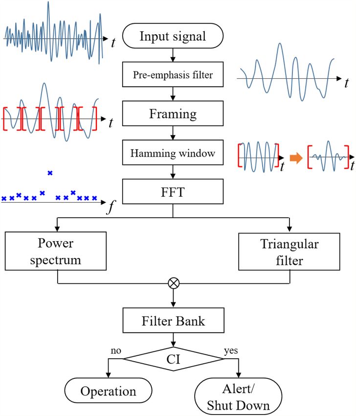
www.nature.com/scientificreports/
Figure 3. While each row distinguishes the calculation domain as time and frequency, each column represents
the DP data before and after a Hamming window. Raw dynamic pressure (a) before the Hamming window in
the time domain, (b) before the Hamming window in the frequency domain (i.e., FFT results), (c) after the
Hamming window in the time domain, and (d) after the Hamming window in the frequency domain (i.e., FFT
results).
Hamming window. DP signals without any windowing process induce discontinuous FFT results at the begin-
ning and end of the signal, which is termed as “leakage error.” A Hamming window can prevent this error in the
FFT analysis55. When a Hamming window is applied on raw DP signals, it can alleviate the discontinuity at both
ends of the frame and attenuate the magnitude of the sidelobes. Figure 3 shows the FFT results before and after
applying the Hamming window to the raw signal. While the first row (Fig. 3a,c) represents the raw data in the
time domain, the second row (Fig. 3b,d) indicates the FFT results in the frequency domain. In addition, whereas
the first column (Fig. 3a,b) describe the results before the Hamming window, the second column (Fig. 3c,d)
represents the results after the Hamming window. The Hamming window is defined by Eq. (4), where N is the
number of data values in a frame.
n
Hamming window, w(n) = 0.54 − 0.46 cos 2π , 0≤n≤N (4)
N
Triangular filter. The main purpose of the triangular filter is to divide the frequency range into sub-frequency
bands, which can efficiently reflect spectral characteristics in a certain band rather than a specific frequency.
In this study, the frequency domain is divided by the Mel-scales in which the frequency resolution is higher at
low frequencies than at high frequencies. As the Mel-scaling converts the linear scale into a logarithmic scale in
frequency, it enables more detailed examination at the low-frequency bands by making the low-frequency band
more sensitive than the high-frequency band. The Mel-scale is defined as
f ′ (n)
Mel-scale: m(n) = 2595 × log10 1 + (5)
700
where n is the number of sub-frequency bands, and f ′ is the modified sub-frequency by the Mel-scaling. The
detailed process for the Mel-scaling is as follows:
First, as the DP data are acquired at 16,000 samples per second in the current study, the frequency range of
the FFT is from 0 to 8000 Hz. We can obtain two Mel-scaled values by inserting the minimum and maximum
frequencies, 0 Hz and 8000 Hz, into Eq. (5), yielding 0 and 2840.
Second, the obtained Mel-scaled range, 0–2840, should be linearly divided into 40 subbands. Here, although
the number of subbands can be varied, we select the number as a commonly used one, 4056. The linearly divided
values are 0, 69.3, 138.5, etc. These calculated values are summarized in Table 4.
Third, the Mel-scaled values are inserted again into the Eq. (5) to determine the corresponding frequency, f ′.
Obviously, the frequency values at the boundaries are 0 Hz and 8000 Hz. The other frequency values are sum-
marized in Table 4.
Lastly, to construct the triangular filter, three frequencies are used from f ′. If the nth frequency, f ′(n), is of
interest, its filter amplitude is set up to be 1, while the amplitude of f ′ (n − 1) and f ′ (n + 1) are 0. This process is
described in Fig. 4. It should be noted that f ′ is different than f obtained from the FFT. Therefore, there can be
several frequencies, f, between f ′ (n − 1) and f ′ (n), or f ′ (n) and f ′ (n + 1). In this case, the filter amplitude for f can
be easily calculated by interpolation between 0 and 1, which is expressed as follows:
Scientific Reports | (2021) 11:3043 | https://doi.org/10.1038/s41598-020-80427-6 6
Vol:.(1234567890)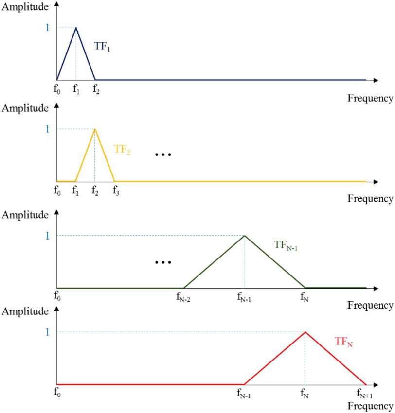
www.nature.com/scientificreports/

                                   m(n) in Eq. (5)       f ’(n) in Eq. (5)          Triangular Filter’s frequency bandwidth
                                             Frequency
                                   m(n)      [mels]      f ’(n)    Frequency [Hz]   f ’(n − 1) – f ’(n + 1) [Hz]
                                   m(0)      0.0         f″0)      0.0              –
                                   m(1)      69.3        f″(1)     44.4             0–91.6
                                   m(2)      138.5       f″(2)     91.6             44.4–141.7
                                   .                     .                          .
                                   .                     .                          .
                                   .                     .                          .
                                   m(39)     2701.5      f′(39)    6993.7           6535–7481.4
                                   m(40)     2770.8      f ’(40)   7481.4           6993.6–8000
                                   m(41)     2840.0      f ’(41)   8000.0           –

                                  Table 4.  Mel-scale conversion chart.

                                  Figure 4.  Mechanism of the triangular filter.

Scientific Reports |   (2021) 11:3043 |                  https://doi.org/10.1038/s41598-020-80427-6                                7

                                                                                                                              Vol.:(0123456789)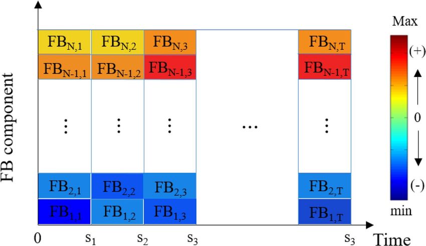
www.nature.com/scientificreports/
Figure 5. Matrix of the magnitude of the FB components.
f < f ′ (n − 1)
0
′
f −f (n−1)
f ′ (n − 1) ≤ f < f ′ (n)
′ (n) ′ (n−1)
f −f
(6)
� �
TFn f = 1 f = f ′ (n)
f ′ (n+1)−f
f ′ (n) < f ≤ f ′ (n + 1)
f ′ (n+1)−f ′ (n)
0 f > f ′ (n + 1)
where TF n f is the magnitude of the nth triangular filter according to frequency f, n is the number of triangular
filters, and f ′ (n) is the calculated frequency with Mel-scaling using Eq. (6).
FB components. The FB component at a specific time interval, t, in the nth bandwidth is obtained by multiply-
ing the result of the power spectrum and the nth triangular filter, as shown in Eq. (7). The calculated FB compo-
nents are represented by the decibel scale to reflect changes in DP in the state of CI. It should be noted that the FB
components are described in the time–frequency domain. In other words, whereas the time interval of interest
is represented on the x-axis, the sub-frequencies are indicated on the y-axis. Therefore, another independent
axis is needed to describe the magnitude of the FB components. In this study, the magnitude is represented by
color bars rather than values on an additional axis, i.e., the z-axis. Figure 5 shows the FB results described above.
FBn,t = (PSn,t × TFn,t ) (7)
where PSn,t and TFn,t are the power spectrum and triangular filter components for the nth subband of the FB at
time t.
As the FB method can display the intensity of CI for every individual subband with respect to time, it is
possible to analyze various frequencies simultaneously (i.e., multi-mode CI). In this study, these particular
characteristics of FB methods have been validated by applying the transition combustion process from a stable
state to an unstable state.
Results and discussion
Combustion instability characteristics of H2/CH4 flames. To grasp the onset of CI from DP signals
during the CI transition process, it is necessary to understand the combustion characteristics of the gas turbine
combustor for various compositions. In this study, the criterion of the onset of CI is set to 0.3 psi as the RMS
value of the DP signal after the FFT, which is equivalent to 2% of the static pressure of the combustion chamber.
This criterion is the most rigorous in comparison to industrial gas turbines, for which the criterion is generally
set to 3–5% of static pressure (SP) of the c ombustor32 (Dawson et al.: 2%31; Lieuwen et al.: 3%32; Rodriguez-
Martinez et al.: 5%33; Lee et al.: 10%34).
Table 5 lists the frequencies, corresponding harmonic modes, and the amplitudes of DP according to the
H2/CH4 ratio and heat input. The frequency and its amplitude corresponding to CI are highlighted in bold. As
the ratio of H2 increases, the CI frequency is shifted to a higher mode. Therefore, transitions of the harmonic
frequencies from the 3rd mode frequency for 12.5–25% H 2 via the 4th mode frequency for 37.5–62.5% H 2 to
Scientific Reports | (2021) 11:3043 | https://doi.org/10.1038/s41598-020-80427-6 8
Vol:.(1234567890)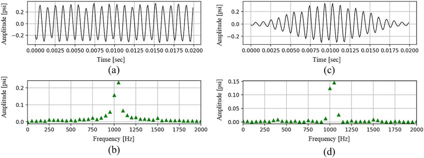
www.nature.com/scientificreports/
40 kW 50 kW
H2:CH4 Frequency [Hz] Amplitude [psi] Frequency [Hz] Amplitude [psi]
0:100 62 0.016 594 0.01
12.5:87.5 763 0.017 788 (3rd mode) 0.445
25:75 763 0.098 804 0.012
37.5:62.5 1015 (4th mode) 0.753 1069 (4th mode) 0.727
50:50 1026 (4th mode) 0.586 1070 (4th mode) 0.912
62.5:37.5 1029 (4th mode) 0.603 1078 (4th mode) 0.857
75:25 1496 (6th mode) 0.319 1590 (6th mode) 0.802
87.5:12.5 710 0.006 1600 (6th mode) 0.541
100:0 702 0.008 1635 0.008
Table 5. Frequencies and corresponding amplitudes of combustion instability with respect to the H
2:CH4 ratio
and heat input.
# Status Fuel composition Heat input ( kW)
Case 1 Stable H2:CH4 = 87.5:12.5
40
Case 2 Unstable H2:CH4 = 75:25
Case 3 Stable H2:CH4 = 100:0
50
Case 4 Unstable H2:CH4 = 87.5:12.5
Table 6. Case study data sets.
the 6th mode frequency for 75–100% H 2 are observed. In addition, as the heat input increases, the amplitude of
DP increases due to the rise of heat release in the combustion zone. This consequently increases the probability
of coupling between fluctuations of the pressure and the heat release rate in the combustion zone54, namely, the
Rayleigh index.
As listed in Table 6 and highlighted in Table 5, two stable cases (Case 1 and Case 3) and two unstable cases
(Case 2 and Case 4) are selected as representative cases using predetermined information for stable and unstable
conditions to compare the effectiveness of the two different methods for CI assessment: TK and FB. In addition,
these cases are used to calculate the detection time in the transition period when changing the fuel composition
(e.g., from Case 1 to Case 2 or from Case 3 to Case 4).
FB analysis of steady‑state CI. As shown in Fig. 6, the time series of the DP and its FFT results for Cases
1–4 are examined to determine the optimal size of the subband. In Cases 1 and 3 (i.e., stable condition), the
peak-to-peak amplitude of the time series DP is under 0.3 psi and the amplitudes in the frequency domain are
also low and show no peak over the entire frequency range. However, in Cases 2 and 4 (i.e., unstable condition),
the peak-to-peak amplitude in the time domain is over 0.3 psi and the amplitudes in the frequency domain are
also quite high and show only one high peak at a specific frequency. As data acquired during 0.02 s sufficiently
represents the main frequencies as well as periodic features of the DP, the size of the subband was set as 0.02 s.
Figure 7 shows the results of FB analysis together with the time series of the DP and TK analysis results for
Cases 1–4. The FB components are calculated from 6400 DP signal samples acquired for 0.4 s after applying the
power spectrum of the FFTs and triangular filter. Subsequently, the criteria of FB components for stable and
unstable status have been calculated from 16,000 DP signals acquired for 1.0 s in stable and unstable H2/CH4
fuel compositions, respectively. The maximum and minimum magnitude of the FB components under stable and
unstable conditions have been determined as the criterion for CI determination. In this study, “under − 85 dB”
and “over − 52 dB” were set as the criterion for stable and an unstable condition, respectively.
The results of FB analysis for Cases 1–4 have been compared with those of the time series of DP and TK analy-
sis, as shown in Fig. 9. In each sub-figure, a – d, the first, second, and third row indicate the time series of the DP,
TK analysis, and FB component, respectively. Furthermore, while Fig. 7a,c show the results obtained from the fuel
compositions causing steady and stable combustion, Fig. 7b,d represent the results from the fuel compositions
causing steady-unstable combustion. In the FB components for Cases 1 and 3 (i.e., the third row in Fig. 7a,c),
the maximum values are − 88 dB at the 23rd subband (bandwidth: 2006.13–2360.09 Hz) and − 94 dB at the 24th
subband (bandwidth: 2177.67–2554.08 Hz), respectively. As the values satisfy the predetermined stable criterion,
i.e., “under − 85 dB,” it can be assessed as a stable condition. However, the maximum FB components for Cases
2 and 4 (i.e., the third row in Fig. 9b,d) are both − 20 dB at the 19th subband (bandwidth: 1450.45–1693.11 Hz).
In these cases, as the value satisfies the unstable criterion, i.e., “over − 52 dB,” it can be determined as unstable.
However, if the FB component lies between − 85 and − 52 dB, it is impossible to assess the combustion status.
Therefore, a single value criterion for CI assessment must be set up instead of two different values, such as − 85 dB
and − 52 dB. To develop the single value criterion, the cut-off time (tcut-off) has been applied to the FB compo-
nent and used as the new criterion for CI assessment. The tcut-off value for the FB component has been defined
Scientific Reports | (2021) 11:3043 | https://doi.org/10.1038/s41598-020-80427-6 9
Vol.:(0123456789)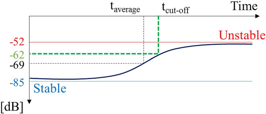
www.nature.com/scientificreports/
Figure 6. Dynamic pressure signal and FFT results (stable, unstable) for each fuel composition. (a) Case 1, (b)
Case 2, (c) Case 3, and (d) Case 4.
√
according to the time when the FB component reaches 1/ 2√of the difference between the stable and unstable
criteria, which implies that the tcut-off is − 62 dB (= (− 85 + 52)/ 2 ) in this s tudy57.
Figure 8 shows a schematic diagram of tcut-off when the FB component changes √ from a stable to an unstable
condition. Based on the definition of the cut-off time, − 62 dB (= (− 85 + 52)/ 2 ) is considered as the new cri-
terion of CI determination. The cut-off time (tcut-off) detects somewhat later than the average time (taverage) of the
two stable/unstable reference values. However, the determination of CI occurrence by tcut-off can be considered
as more precise if we consider the possibility of returning to a stable flame during the transition process.
Performance comparison of TK and FB during transient condition. Figures 9a and 10a show the
time series DP signals during the CI transition from stable to unstable conditions (Case 1 → Case 2, and Case
3 → Case 4). The signal is acquired for 3.0 s such that 48,000 DP samples are obtained. As previously mentioned,
if the RMS of the DP signal exceeds 2% of the static pressure, it can be judged that CI has occurred. Based on the
2% criterion, the CI onset time is determined to be 2.33 s for the transition of Case 1 → Case 2 and 2.63 s for the
transition of Case 3 → Case 4.
The CI assessment results using three different methods (i.e., RMS, TK, and FB) in the status transition have
been compared in view of the detection time and accuracy, as shown in Figs. 9 and 10. Initially, if we apply the
RMS criterion for CI assessment (i.e., exceeding 2% of the static pressure in a combustor), the CI onset time is
detected as 2.33 s for the transition of Case 1 → Case 2, and 2.63 s for the transition of Case 3 → Case √
4. When the
method is changed from RMS to TK, a new criterion for CI assessment has been set as 1.94 (= 3 − 1.5/ 2) accord-
ing to the definition of the cut-off time. The detection time from TK is 2.05 s for Case 1 → Case 2, and 2.43 s for
Case 3 → Case 4, which is much earlier than for the RMS method. If we use the FB method, the detection time
for the two cases is 2.03 and 2.41 s. The FB method shows comparable results for RMS and TK. Although the
difference from TK in detection time is as small as 0.4 s, such a small leading time can be very meaningful for
the monitoring system operated by automatic electronic control units. Next, in view of the accuracy, the RMS
methods detects the CI at 2.33 s and 2.63 s, respectively, for Case 1 → Case 2, and Case 3 → Case 4. However, in
Fig. 10, the first peak of pressure is observed at approximately 0.7 s. The RMS method does not detect the first
peak, but the TK method does. As shown in Fig. 10b, the TK value is below the criterion of 0.63 s, which implies
Scientific Reports | (2021) 11:3043 | https://doi.org/10.1038/s41598-020-80427-6 10
Vol:.(1234567890)www.nature.com/scientificreports/
Figure 7. Dynamic pressure signal, temporal kurtosis, and FB components for each fuel composition. (a)
Bstable = 23rd (− 88 dB), (b) FBunstable = 19th (− 20 dB), (c) FBunstable = 24th (− 94 dB), and (d) FBstable = 19th
F
(− 20 dB).
Figure 8. Determination of the cut-off time to obtain early alert for combustion instability.
that TK detects the CI at this time. Such sensitive as well as early detection is the strong aspect of the TK analysis
method. However, TK shows disadvantages in that the values at each frequency (i.e., asterisk marks in Figs. 9b
and 10b) fluctuate too much. Although linear regression has been applied to TK in order to alleviate the effect
of the outlier values, TK shows more fluctuation than RMS or FB, as shown in Figs. 9 and 10.
Scientific Reports | (2021) 11:3043 | https://doi.org/10.1038/s41598-020-80427-6 11
Vol.:(0123456789)www.nature.com/scientificreports/
Figure 9. CI analysis results using (a) RMS, (b) TK, and (c) FB for transition from Case 1 to Case 2.
The TK values are 3.37 at 0.22 s in Fig. 9b and 3.51 at 1.68 s in Fig. 10b, respectively, which exceeds the stable
reference of 3.0 as the theoretical maximum value of TK in a stable condition. In the frame at 1.68 s in Fig. 10b,
the DP signal histogram, as shown in Fig. 11, has a stable normal distribution that is centered at 0.0, but there
is an outlier signal that has a magnitude of 0.11 psi. According to the definition of TK, the quadratic term of the
numerator with an outlier has a great influence in determining the value of TK. Even though the data points are
ordered around the unstable criterion during the CI, several TK values exceed the stable reference of 3.0 during
stable conditions. Therefore, the large fluctuation of TK in the stable regime can cause the false-positive detection
by approaching the CI criterion of TK.
FB detects not only the 19th subband (bandwidth: 1450.45–1693.11 Hz) but also the other frequencies, such
as 27th (bandwidth: 2760.36–3212.98 Hz), as shown in Figs. 9c and 10c. Herein, the second subband frequency
is the higher harmonic mode of the 19th subband, which has multi-mode frequencies. However, TK cannot
show the various CI frequencies occurring simultaneously because it is performed using only the main lobe of
the CI frequency. Therefore, the detection of multi-modes of CI can be ensured only through the FB method.
The drawback of the FB method is that the criterion of FB can differ according to the combustor type and
operation conditions because the signal characteristics and frequency bands vary depending on the type of
combustor. Furthermore, the criterion also varies according to the sampling rate of the DP signal and frame
size. However, if the magnitude of the FB component is initially set up for stable and unstable flames, the FB
method can be used as an additional indicator of detection of CI for a monitoring system or combustion tuning
procedure.
Post‑processing computation time. Although the detection time of the onset of CI is calculated cor-
rectly using each method, it can be an inefficient method if it requires more time for data collection and calcu-
lation for post processing. The optimal number of DP signals in the present study is 320, and it takes 20 ms to
acquire one frame. The DP data acquired for 3 s is divided into 150 frames to calculate the averaged computation
time (tcom) of post-processing for each frame because the DP data for 1 s consists of the sum of 50 frames.
Scientific Reports | (2021) 11:3043 | https://doi.org/10.1038/s41598-020-80427-6 12
Vol:.(1234567890)www.nature.com/scientificreports/
Figure 10. CI analysis results using (a) RMS, (b) TK, and (c) FB for transition from Case 3 to Case 4.
Figure 12 shows the results of each tcom (first–third quartile with whiskers from the minimum to maximum)
by performing 100 iterative calculations in consideration of the deviation of the time to load the DP signal
from the library in the Python program. The t com values from the RMS, TK, and FB methods are 1.529 ms,
1.605 ms, and 1.681 ms, respectively. It requires only 7.6%, 8.0%, and 8.4%, respectively, of the time to acquire
the dynamic signals of one frame. Therefore, it takes much more time to acquire the DP data rather than to
evaluate the combustion state or CI onset. The tcom value of the FB method is lower than that of the RMS and TK
methods. Nevertheless, the relatively slow computation time has little effect on evaluating the combustion state
and detection time of CI because it takes only 0.38% more time when compared to the data acquisition time. In
fact, the detection time of CI using the FB method is up to 300 ms (15 frames) faster than the other methods.
Therefore, the FB method, which is proposed in the present study, can be an effective diagnostic tool of CI for
a gas turbine combustor.
Conclusion
In this study, the FB method was introduced as a potential indicator that can detect CI in a model gas turbine
combustor. Combustion experiments were carried out in a partially premixed combustor for various fuel compo-
sitions of H
2 and C
H4. The performance of FB together with RMS and TK were compared during the CI transition
process from the perspectives of accuracy, detection time, and multi-mode detection possibility. Based on the
results, we can conclude the following.
1. The CI detection time of RMS, TK, and FB are summarized in Table 7. FB and TK show the comparable
performance in CI detection time with the RMS method. In terms of detection sensitivity, RMS cannot detect
weak CI, but TK and FB show sensitive and accurate performance in detecting weak CI. Herein, it should be
Scientific Reports | (2021) 11:3043 | https://doi.org/10.1038/s41598-020-80427-6 13
Vol.:(0123456789)www.nature.com/scientificreports/
Figure 11. Detailed analysis of the DP signal with an outlier. (a) Magnitude (b) histogram of DP.
noted that the RMS method is also more sensitive if the criterion of RMS is set to be lower. Thus, it is difficult
to definitively state that FB methodology is superior to the existing methodologies of RMS or TK.
2. However, a lower criterion will increase the probability of false-positive warnings of CI, so that the use of
multiple precursors is recommended to enhance the robustness of prediction of onset of CI. That is, FB can
complement other measures in detecting the onset of CI and, in this manner, it would allow one to avoid
false-positive or even false-negative warnings.
3. TK is a signal-processing method based on a single CI frequency, but FB calculates the power spectrum in the
entire frequency domain over time. Therefore, the FB method has an advantage in multi-mode CI detection
as well as single-mode CI detection that usually occurs from H 2/CH4 flames in a combustor.
Scientific Reports | (2021) 11:3043 | https://doi.org/10.1038/s41598-020-80427-6 14
Vol:.(1234567890)www.nature.com/scientificreports/
Figure 12. Box plot of the post-processing computation time of each CI assessment method.
Case 3 → Case 4
# Case 1 → Case 2 [s] First peak [s] Second peak [s]
RMS 2.33 No detection 2.63
TK 2.05 0.63 2.43
FB 2.03 0.61 2.41
Table 7. Summary of detection times using RMS, TK, and FB.
Received: 24 April 2020; Accepted: 22 December 2020
References
1. Zhao, D., Guan, Y. & Reinecke, A. Characterizing hydrogen-fuelled pulsating combustion on thermodynamic properties of a
combustor. Commun. Phys. 2, 44 (2019).
2. Crippa, M. et al. High resolution temporal profiles in the emissions database for global atmospheric research. Sci. Data 7, 121
(2020).
3. Krishnamoorthi, M., Malayalamurthi, R., He, Z. & Kandasamy, S. A review on low temperature combustion engines: Performance,
combustion and emission characteristics. Renew. Sustain. Energy Rev. 116, 109404 (2019).
4. Ruan, C. et al. Principles of non-intrusive diagnostic techniques and their applications for fundamental studies of combustion
instabilities in gas turbine combustors: A brief review. Aerosp. Sci. Technol. 84, 585–603 (2019).
5. Rao, K., Karmakar, S. & Basu, S. Atomization characteristics and instabilities in the combustion of multi-component fuel droplets
with high volatility differential. Sci. Rep. 7, 8925 (2017).
6. Santana, A. Passive control of combustion instability: Practical application of acoustic devices to suppress combustion instability in
chambers. (LAP LAMBERT Academic Publishing, 2010).
7. Yang, D., Laera, D. & Morgans, A. S. A systematic study of nonlinear coupling of thermoacoustic modes in annular combustors.
J. Sound Vib. 456, 137–161 (2019).
8. Han, X. et al. Inlet temperature driven supercritical bifurcation of combustion instabilities in a lean premixed prevaporized com-
bustor. Exp. Therm. Fluid Sci. 109, 109857 (2019).
9. Kobayashi, H., Gotoda, H. & Tachibana, S. Nonlinear determinism in degenerated combustion instability in a gas-turbine model
combustor. Phys. A 510, 345–354 (2018).
10. Park, S., Choi, G. & Tanahashi, M. Combustion characteristics of syngas on scaled gas turbine combustor in pressurized condition:
Pressure, H2/CO ratio, and N 2 dilution of fuel. Fuel Process. Technol. 175, 104–112 (2018).
11. Park, S., Min, G. & Tanahashi, M. Demonstration of a gas turbine combustion-tuning method and sensitivity analysis of the
combustion-tuning parameters with regard to NOx emissions. Fuel 239, 1134–1142 (2019).
12. Lee, M. C., Yoon, J., Joo, S. & Yoon, Y. Gas turbine combustion characteristics of H2/CO synthetic gas for coal integrated gasifica-
tion combined cycle applications. Int. J. Hydrogen Energy 40, 11032–11045 (2015).
13. Joo, S., Yoon, J., Kim, J., Lee, M. & Yoon, Y. NOx emissions characteristics of the partially premixed combustion of H2/CO/CH4
syngas using artificial neural networks. Appl. Therm. Eng. 80, 436–444 (2015).
Scientific Reports | (2021) 11:3043 | https://doi.org/10.1038/s41598-020-80427-6 15
Vol.:(0123456789)www.nature.com/scientificreports/
14. Wu, G., Lu, Z., Guan, Y., Li, Y. & Ji, C. Z. Characterizing nonlinear interaction between a premixed swirling flame and acoustics:
Heat-driven acoustic mode switching and triggering. Energy 158, 546–554 (2018).
15. Palies, P., Durox, D., Schuller, T. & Candel, S. The combined dynamics of swirler and turbulent premixed swirling flames. Combust.
Flame 157, 1698–1717 (2010).
16. Ji, C., Zhao, D., Li, X., Li, S. & Li, J. Nonorthogonality analysis of a thermoacoustic system with a premixed V-shaped flame. Energy
Convers. Manag. 85, 102–111 (2014).
17. Zhang, Z. et al. Transient energy growth of acoustic disturbances in triggering self-sustained thermoacoustic oscillations. Energy
82, 370–381 (2015).
18. Kobayashi, T., Murayama, S., Hachijo, T. & Gotoda, H. Early detection of thermoacoustic combustion instability using a methodol-
ogy combining complex networks and machine learning. Phys. Rev. Appl. 11, 64034 (2019).
19. Nair, V., Thampi, G., Karuppusamy, S., Gopalan, S. & Sujith, R. I. Loss of chaos in combustion noise as a precursor of impending
combustion instability. Int. J. Spray Combust. Dyn. 5, 273–290 (2013).
20. Tsoutsanis, E., Meskin, N., Benammar, M. & Khorasani, K. A dynamic prognosis scheme for flexible operation of gas turbines.
Appl. Energy 164, 686–701 (2016).
21. Li, Y. G. & Nilkitsaranont, P. Gas turbine performance prognostic for condition-based maintenance. Appl. Energy 86, 2152–2161
(2009).
22. Rouwenhorst, D. & Hermann, J. Precursor for thermoacoustic stability in annular combustion systems, based on output-only
system identification. In EVI-GTI and PIWG Joint Conference on Gas Turbine Instrumentation, 1–5 (2016) https: //doi.org/10.1049/
cp.2016.0835.
23. De, S., Agarwal, A. K., Chaudhuri, S. & Sen, S. Modeling and Simulation of Turbulent Combustion (Springer, Singapore, 2018).
24. Noiray, N. Linear growth rate estimation from dynamics and statistics of acoustic signal envelope in turbulent combustors. J. Eng.
Gas Turbines Power 139, (2016).
25. Lieuwen, T. Online combustor stability margin assessment using dynamic pressure data. J. Eng. Gas Turbines Power 127, 478–482
(2005).
26. Tongxun, Y. & Gutmark, E. J. Online prediction of the onset of combustion instability based on the computation of damping ratios.
J. Sound Vib. 310, 442–447 (2008).
27. Stadlmair, N. V., Hummel, T. & Sattelmayer, T. Thermoacoustic damping rate determination from combustion noise using Bayesian
statistics. In Proceedings of the ASME Turbo Expo 1–11 (2017). https://doi.org/10.1115/GT201763338.
28. Kabiraj, L. & Sujith, R. I. Nonlinear self-excited thermoacoustic oscillations: Intermittency and flame blowout. J. Fluid Mech. 713,
376–397 (2012).
29. Guan, Y., Liu, P., Jin, B., Gupta, V. & Li, L. K. B. Nonlinear time-series analysis of thermoacoustic oscillations in a solid rocket
motor. Exp. Therm. Fluid Sci. 98, 217–226 (2018).
30. Murayama, S., Kinugawa, H., Tokuda, I. T. & Gotoda, H. Characterization and detection of thermoacoustic combustion oscillations
based on statistical complexity and complex-network theory. Phys. Rev. E 97, 22223 (2018).
31. Dawson, J. R., Rodriguez-Martinez, V. M., Syred, N. & O’Doherty, T. The effect of combustion instability on the structure of
recirculation zones in confined swirling flames. Combust. Sci. Technol. 177, 2349–2371 (2005).
32. Lieuwen, T. C. Experimental investigation of limit-cycle oscillations in an unstable gas turbine combustor. J. Propuls. Power 18,
61–67 (2002).
33. Rodriguez-Martinez, V. M., Dawson, J. R., O’Doherty, T. & Syred, N. Low-frequency combustion oscillations in a swirl burner/
furnace. J. Propuls. Power 22, 217–221 (2006).
34. Lee, S. Y., Seo, S., Broda, J. C., Pal, S. & Santoro, R. J. An experimental estimation of mean reaction rate and flame structure during
combustion instability in a lean premixed gas turbine combustor. Proc. Combust. Inst. 28, 775–782 (2000).
35. Song, W. & Cha, D. Temporal kurtosis of dynamic pressure signal as a quantitative measure of combustion instability. Appl. Therm.
Eng. 104, 577–586 (2016).
36. Choi, J., Choi, O., Lee, M. C. & Kim, N. On the observation of the transient behavior of gas turbine combustion instability using
the entropy analysis of dynamic pressure. Exp. Therm. Fluid Sci. 115, 110099 (2020).
37. Gopalakrishnan, E. A., Sharma, Y., John, T., Dutta, P. S. & Sujith, R. I. Early warning signals for critical transitions in a thermoa-
coustic system. Sci. Rep. 6, 35310 (2016).
38. Tsai, F. F., Fan, S. Z., Cheng, H. L. & Yeh, J. R. Multi-timescale phase-amplitude couplings in transitions of anesthetic-induced
unconsciousness. Sci. Rep. 9, 1–11 (2019).
39. Biem, A., Katagiri, S., Mcdermott, E. & Juang, B. An application of discriminative feature extraction to filter-bank-based speech
recognition. IEEE Trans. Speech Audio Process. 9, 96–110 (2001).
40. Silva, J., Member, S. & Narayanan, S. S. Discriminative wavelet packet filter bank selection for pattern recognition. IEEE Trans.
Signal Process. 57, 1796–1810 (2009).
41. Giilzow, T., Engelsberg, A. & Heute, U. Comparison of a discrete wavelet transformation and a nonuniform polyphase filterbank
applied to spectral-subtraction speech enhancement. Signal Process. 64, 5–19 (1998).
42. Sainath, T. N. et al. Learning filter banks within a deep neural network framework. In 2013 IEEE Work. Autom. Speech Recognit.
Underst. 297–302 (2013) https://doi.org/10.1109/ASRU.2013.6707746.
43. Fedurek, P., Zuberbühler, K. & Dahl, C. D. Sequential information in a great ape utterance. Sci. Rep. 6, 1–11 (2016).
44. Chien, Y. W. et al. An automatic assessment system for Alzheimer’s disease based on speech using feature sequence generator and
recurrent neural network. Sci. Rep. 9, 1–10 (2019).
45. Abdouni, A., Vargiolu, R. & Zahouani, H. Impact of finger biophysical properties on touch gestures and tactile perception: Aging
and gender effects. Sci. Rep. 8, 1–13 (2018).
46. Duque, D., Wang, X., Nieto-Diego, J., Krumbholz, K. & Malmierca, M. S. Neurons in the inferior colliculus of the rat show stimulus-
specific adaptation for frequency, but not for intensity. Sci. Rep. 6, 1–15 (2016).
47. Angello L. Tuning approaches for DLN combustor performance and reliability. EPRI, Palo Alto, CA, 1005037. 11249874(2005).
Tuning approaches for DLN combustor performance and reliability. Electr. Power Res. Inst. (2006)
48. Lee, M. C. et al. Investigation into the cause of high multi-mode combustion instability of H2/CO/CH4 syngas in a partially pre-
mixed gas turbine model combustor. Proc. Combust. Inst. 35, 3263–3271 (2015).
49. Taamallah, S. et al. Fuel flexibility, stability and emissions in premixed hydrogen-rich gas turbine combustion: Technology, fun-
damentals, and numerical simulations. Appl. Energy 154, 1020–1047 (2015).
50. Kim, Y. J., Yoon, Y. & Lee, M. C. On the observation of high-order, multi-mode, thermo-acoustic combustion instability in a model
gas turbine combustor firing hydrogen containing syngases. Int. J. Hydrogen Energy 44, 11111–11120 (2019).
51. Sampath, R. & Chakravarthy, S. R. Investigation of intermittent oscillations in a premixed dump combustor using time-resolved
particle image velocimetry. Combust. Flame 172, 309–325 (2016).
52. Christoph, B. & Bernd, P. Permutation entropy: A natural complexity measure for time series. Phys. Rev. Lett. 88, 174102 (2002).
53. Champagne, F. H. & Kromat, S. Experiments on the formation of a recirculation zone in swirling coaxial jets. Exp. Fluids 29,
494–504 (2000).
54. Yoon, J., Lee, M., Joo, S., Kim, J. & Yoon, Y. Instability mode and flame structure analysis of various fuel compositions in a model
gas turbine combustor. J. Mech. Sci. Technol. 29, 899–907 (2015).
Scientific Reports | (2021) 11:3043 | https://doi.org/10.1038/s41598-020-80427-6 16
Vol:.(1234567890)www.nature.com/scientificreports/
55. Kumar, S., Singh, K. & Saxena, R. Analysis of dirichlet and generalized ‘Hamming’ window functions in the fractional Fourier
transform domains. Signal Process. 91, 600–606 (2011).
56. Mendes, T. M., Duque, C. A., Silva, L. R. M., Ferreira, D. D. & Meyer, J. Supraharmonic analysis by fi lter bank and compressive
sensing. Electr. Power Syst. Res. 169, 105–114 (2019).
57. Mondragón, R. J. Estimating degree–degree correlation and network cores from the connectivity of high–degree nodes in complex
networks. Sci. Rep. 10, 5668 (2020).
Acknowledgements
This work was supported by the National Research Foundation of Korea (NRF) grant funded by the Korea
government (MSICT) (No. NRF-2019R1C1C1009739). This research was supported by Korea Electric Power
Corporation (Grant number: R20XO02-34).
Author contributions
S.J.: conceptualization, methodology, formal analysis, investigation, data curation, writing—original draft. J.C.:
conceptualization, methodology, formal analysis, investigation, data curation, writing—original draft. N.K.:
formal analysis, investigation, writing—review and editing, supervision. M.C.L.: validation, formal analysis,
investigation, writing—review and editing.
Competing interests
The authors declare no competing interests.
Additional information
Correspondence and requests for materials should be addressed to N.K. or M.C.L.
Reprints and permissions information is available at www.nature.com/reprints.
Publisher’s note Springer Nature remains neutral with regard to jurisdictional claims in published maps and
institutional affiliations.
Open Access This article is licensed under a Creative Commons Attribution 4.0 International
License, which permits use, sharing, adaptation, distribution and reproduction in any medium or
format, as long as you give appropriate credit to the original author(s) and the source, provide a link to the
Creative Commons licence, and indicate if changes were made. The images or other third party material in this
article are included in the article’s Creative Commons licence, unless indicated otherwise in a credit line to the
material. If material is not included in the article’s Creative Commons licence and your intended use is not
permitted by statutory regulation or exceeds the permitted use, you will need to obtain permission directly from
the copyright holder. To view a copy of this licence, visit http://creativecommons.org/licenses/by/4.0/.
© The Author(s) 2021
Scientific Reports | (2021) 11:3043 | https://doi.org/10.1038/s41598-020-80427-6 17
Vol.:(0123456789)You can also read