A Parameterized Linear Magnetic Equivalent Circuit for Analysis and Design of Radial Flux Magnetic Gears-Part I: Implementation
←
→
Page content transcription
If your browser does not render page correctly, please read the page content below
1

          A Parameterized Linear Magnetic Equivalent
          Circuit for Analysis and Design of Radial Flux
             Magnetic Gears–Part I: Implementation
           Matthew Johnson, Member, IEEE, Matthew C. Gardner, Student Member, IEEE, Hamid A. Toliyat,
                                                Fellow, IEEE

                                                                              magnetically geared systems offer the potential to combine the
    Abstract--Magnetic gears offer a promising alternative to                 compact size and cost effectiveness of mechanically geared
mechanical gears with the added benefit of contactless power                  systems with the reliability of direct drive machines.
transfer. However, quick and accurate analysis tools are                      Additionally, several different magnetically geared machine
required to optimize magnetic gear designs and commercialize
                                                                              topologies integrate a magnetic gear directly with a higher
the technology. Therefore, this work proposes an extremely fast
and accurate 2D Magnetic Equivalent Circuit (MEC) model of                    speed motor or generator to produce a single extremely
radial flux magnetic gears with surface mounted magnets. This                 compact device capable of directly interfacing with a lower
MEC model’s distinguishing characteristics include a heavily                  speed, higher torque load or prime mover [5], [6]. Therefore,
parameterized gear geometry and a parametrically adjustable                   magnetic gears have received interest for use in a wide variety
systematic flux tube distribution which allow for accurate and                of applications such as wind turbines [7], wave energy
efficient analysis of a wide array of designs. Furthermore, the
                                                                              harvesting [8], electric vehicles [6], and electric ships [9].
model is fully linear which results in very quick simulation run
times without sacrificing significant torque prediction accuracy                 Nonetheless, magnetic gears still struggle to compete with
for most practical designs. This is Part I of a two part paper and            their mechanical counterparts and achieve parity or superiority
focuses on the implementation of the MEC model. Part II                       with respect to crucial fundamental considerations such as
validates the accuracy of the MEC model by comparing its                      size, weight, and cost [10]. For this technology to realize the
torque and flux density predictions with those produced by                    full extent of its potential advantages, it is necessary to be able
nonlinear Finite Element Analysis (FEA).
                                                                              to perform extensive, application specific parametric
   Index Terms--finite element analysis, magnetic equivalent
                                                                              optimizations [11]. This requires fast and accurate analysis
circuit, magnetic gear, optimization, permeance network, radial               tools capable of characterizing the performance of numerous
flux, reluctance network, torque density.                                     parametric design variations. The basic tools commonly used
                                                                              for evaluation of electromechanical devices include finite
                          I. INTRODUCTION                                     element analysis (FEA) models, analytical models, winding

O     VER the past two decades, magnetic gears have received                  function theory, and magnetic equivalent circuit (MEC)
      significant attention as an intriguing alternative to                   models, all of which can be applied to magnetic gears. While
traditional mechanical gears [1]-[4].        Magnetic gears                   FEA models are generally very accurate, robust, and flexible,
accomplish the same fundamental behavior as mechanical                        analytical and winding function theory models are much faster
gears. However, magnetic gears rely on the modulated                          than FEA but less accurate and less flexible. MEC models
interaction of fluxes generated by permanent magnets (PMs)                    represent a compromise between the accuracy and flexibility
on the rotors, instead of mechanical contact between the                      of FEA models and the speed of analytical models.
moving components. This provides a plethora of potential                         The basic concept of an MEC (also known as a reluctance
advantages, including inherent overload protection, reduced                   network) is to decompose a physical electromagnetic system
maintenance requirements, decreased acoustic noise, and                       into flux tubes (defined paths through which magnetic flux
physical isolation between the input and output shafts. Thus,                 flows) and represent each tube using lumped reluctances,
                                                                              magnetomotive force (MMF) sources, and flux sources to
    M. Johnson is with the Advanced Electric Machines and Power               collectively form a lumped parameter magnetic equivalent
Electronics Lab in the Department of Electrical and Computer Engineering at   circuit, which is directly analogous to a traditional lumped
Texas A&M University, College Station, TX 77843 USA (e-mail:                  parameter electrical circuit and can be solved using the same
mjohnson11@tamu.edu).
    M. C. Gardner is with the Advanced Electric Machines and Power            set of analysis techniques. Just as Kirchhoff’s current and
Electronics Lab in the Department of Electrical and Computer Engineering at   voltage laws define the system of equations for an electrical
Texas A&M University, College Station, TX 77843 USA (e-mail:                  circuit, Gauss’s law for magnetism and Ampere’s circuital law
gardner1100@tamu.edu).
    H. A. Toliyat is with the Advanced Electric Machines and Power            define the corresponding system of equations for MECs.
Electronics Lab in the Department of Electrical and Computer Engineering at      Although MEC and FEA models both analyze a system by
Texas A&M University, College Station, TX 77843 USA (e-mail:                  breaking it up into pieces of varying sizes, there are some
toliyat@tamu.edu).

© 2017 IEEE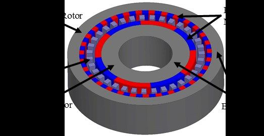
2
critical differences between the two approaches. The most
significant distinction is that flux flow directions are
predetermined in MEC models by the definition of the flux
tubes, but in FEA models the flux orientation in each element
is only determined as a result of the model solution. Thus,
MEC models typically, although not universally, use scalar
quantities such as MMFs (scalar magnetic potentials) or scalar
fluxes as the unknown state variables, whereas FEA models
commonly use vector quantities, such as vector magnetic
potentials. Additionally, MEC models traditionally rely
heavily on prior empirical knowledge of system behavior and
Fig. 1. Radial flux magnetic gear with surface permanent magnets.
use significantly fewer elements than FEA models; however,
this difference is not necessarily an intrinsic characteristic of
Although MECs have been used extensively to model
the two approaches.
various types of electric machines, there are only a few
The concepts of a magnetic circuit and reluctance date back
instances in which the concept has been applied to the analysis
well into the 1800s [12]. Furthermore, Hopkinson’s Law,
of rotary magnetic gears and magnetically geared machines
F = RΦ (1) [28]-[31] or linear magnetic gears [32]. Furthermore, while
[28]-[31] do demonstrate the potential for MEC models to
was formulated by 1886 and relates the scalar magnetic
evaluate a gear design much more rapidly than FEA models,
potential or MMF, F, drop across a flux tube to the magnetic
they use extremely coarse reluctance networks with very few
flux, Φ, flowing through the flux tube and the reluctance, R, elements in the MEC. Also, they provide no analysis of the
of the flux tube. Since that time, there have been several MEC discretization’s impact on its accuracy and little
studies demonstrating the ability of MEC models to analyze indication of how the MEC’s accuracy varies with different
both induction motors and various synchronous machines, design parameters. Additionally, only the work in [30] offers
often with better accuracy than simplified analytical models limited discussion of a 3D MEC model with very few
and significantly faster simulation run times than elements included to account for axial leakage flux. This
corresponding FEA models [13]-[24]. A few works have also study uses an approach more in line with the MEC models
established that MEC techniques are well suited for adaptation developed in [18], [19], [22], and [24]-[27], in the sense that it
to 3D models, with their advantages of reduced computational systematically creates a fully parameterized flux tube mesh by
intensity and faster simulation times becoming even more breaking the magnetic gear up into pieces, referred to as node
pronounced as compared to 3D FEA models [25]-[27]. cells. The levels of discretization in different regions of the
This is Part I of a two part study of a generalized, gear are parameterized so that more mesh elements can be
parametric linear MEC model for analysis of the coaxial radial added to the areas that need high resolution for accuracy and
flux magnetic gear topology with surface mounted permanent fewer elements can be used in the other regions to minimize
magnets shown in Fig. 1. The coaxial magnetic gear simulation run times. Finally, whereas [28]-[31] all develop at
possesses three rotors: the high speed permanent magnet rotor least partially nonlinear models, this work employs a fully
(HSR), the low speed permanent magnetic rotor (LSR), and linear MEC model that assumes a constant permeability for
the intermediate ferromagnetic modulator rotor. The both the modulators and the back irons. The evaluation
relationship between the number of permanent magnet pole presented in Part II demonstrates that the linear model is still
pairs and the number of modulators is given by extremely accurate for analysis of the torque capabilities of
QM = PHS + PLS (2) most reasonable ideal designs, as suggested by the results in
[32]. This occurs because the large linear reluctances of the
where PHS is the number of pole pairs on the HSR, PLS is the two sets of magnets and the two air gaps dominate the much
number of pole pairs on the LSR, and QM is the number of smaller nonlinear reluctances of the back irons and
modulators. If the modulators are fixed, the speeds of the modulators, even if the back irons and modulators experience
HSR and LSR are related by the gear ratio according to significant saturation. The linear model allows for
HS − PLS tremendously fast calculation of a gear design’s torque
Gear Ratio =0
= = (3) capabilities. Furthermore, the MEC implementation, which is
Mods LS PHS
described in the following section, is well suited for extension
where ωHS, ωLS, and ωMods are the speeds of the HSR, LSR, and to a nonlinear model using an iterative approach such as the
modulators, respectively. Alternatively, if the LSR is fixed one described in [33]. This extension to a nonlinear model is
and the modulators rotate instead, then the gear ratio becomes only necessary for analysis of additional considerations, such
positive and increases in magnitude by one to as losses or flux densities in the air regions beyond the rotor
back irons, or designs which include features, such as a
HS Q modulator bridge, that significantly increase the system’s
Gear Ratio =0
= = M . (4)
LSR Mods PHS nonlinearity.
© 2017 IEEE
3
II. THE NODE CELL where A represents the cross-sectional area of the flux tube
The 2D MEC mesh is systematically formed by dividing surface normal to the flux path, μ is the permeability of the
the magnetic gear cross-section into radial and circumferential physical material that comprises the flux tube, and l is the total
(tangential or angular) layers as illustrated by the simple length of the flux tube flux path. Using these relationships,
example shown in Fig. 2, which depicts a source free annular the permeances of each radially directed flux tube (Prad) and
region in the r-θ plane, divided into 3 radial layers (RL) along each tangentially directed flux tube (Ptan) in the reluctance
the r dimension and 8 angular layers (AL) along the θ network mesh can be calculated according to the following
dimension. Each intersection of a radial layer and an angular formulas:
layer defines an annular sector, referred to as a 2D node cell.
−1
Every 2D node cell consists of two radially directed rout dr z
reluctances and two tangentially directed reluctances, each of
Prad =
rin
z (r)
=
ln(rout rin )
(6)
which is connected to the center node of the cell and one of
the cell’s radial or tangential boundaries as shown in Fig. 2. rout zdr z rout
Each of these lumped reluctances corresponds to a flux tube
oriented along the same direction, which allows flux to flow in
Ptan = rin
= ln
(r ) rin
.
(7)
a positive or negative direction along the specified path. In In each of these equations, rin indicates the inner radius of the
this study, the MEC model is solved using node MMF analysis flux tube, rout denotes the outer radius of the flux tube, Δθ is
(which is analogous to node voltage analysis in electrical the uniform angular width of the flux tube (in radians), Δz is
circuits), based on Gauss’s law for magnetism, in which the the uniform axial height of the flux tube (which corresponds to
scalar magnetic potentials at each node represent the unknown the full axial height of the system in a 2D model or the axial
state variables. Therefore, it is more appropriate to use height of the axial layer in a 3D model), and μ is the
lumped permeances rather than their multiplicative inverses, permeability of the flux tube material. If a flux tube overlaps
lumped reluctances. An alternate 2D MEC model with two different materials, the flux tube is divided into two
implementation based on mesh flux analysis techniques parts, one for each material region, and the lumped
derived from Ampere’s circuital law was also developed using permeances for each part are calculated and then combined in
fluxes as the unknown state variables, but the node MMF series or parallel, using the same formulas employed for
approach was ultimately selected for ease of extension to a 3D combining series or parallel conductances in electrical circuits.
model, which has already been implemented and will be Conceptual illustrations of radially and tangentially oriented
presented in a future paper. However, while the node flux tubes are provided in Fig. 3(a) and Fig. 3(b), respectively.
potential and mesh flux approaches are essentially Note that each radially directed flux tube corresponds to one
computationally equivalent for a linear model, the mesh flux radial half of its node cell, the full angular width of its node
methodology may prove to be computationally advantageous cell, and the full axial height of its node cell. Equation (6)
when extending the MEC to a nonlinear model [34]. uses integration to calculate the total lumped radial permeance
by combining the reluctances of series connected differential
radial slivers of the flux tube. Similarly, each tangentially
directed flux tube corresponds to the full radial width of its
node cell, one angular half of its node cell, and the full axial
height of its node cell. Equation (7) uses integration to
combine the permeances of parallel connected differential
radial slivers of the flux tube.
Fig. 2. Definition of mesh node cells based on intersection of radial and (a) (b)
angular layers. Fig. 3. Conceptual illustrations of (a) radially and (b) tangentially oriented
flux tubes.
The lumped permeance of a uniform flux tube is given by
The appropriate lumped parameter representations of flux
1 A tubes corresponding to permanent magnets can be derived by
P= = (5)
R l analyzing the linear 2nd quadrant permanent magnet B-H
curve shown in Fig. 4 and the corresponding linear equation
© 2017 IEEE
4
BPM = PM H PM + Br (8)
where BPM and HPM are the magnetic flux density and the
magnetic field strength in the permanent magnet, Br is its
remanence or residual flux density, Hc is its coercivity, and
μPM is its recoil permeability defined according to
Br
PM = . (9)
Hc
Only radially magnetized permanent magnets, and thus only
radially oriented flux tubes within permanent magnets are
Fig. 4. Linear 2nd quadrant permanent magnet B-H curve.
considered in this analysis; however, the same process can
easily be extended to permanent magnets with tangential or
axial magnetization components for analysis of other magnet
configurations such as Halbach arrays or axially oriented
systems. Ultimately, the flux tube can be represented by
either of the equivalent circuit configurations in Fig 5(a) or
Fig 5(b), which are analogous to Thévenin and Norton
equivalent circuits, respectively. In both cases, Prad is the
permeance of the radial flux tube assuming a permeability of (a) (b)
μPM. The equivalent MMF and flux injected by the magnet, Fig. 5. (a) Thévenin and (b) Norton equivalent circuit representations of
Finj and Φinj, respectively, are given by radially oriented permanent magnet flux tubes.
Br
Finj = − (rout − rin ) (10)
PM
Finj
inj = . (11)
R rad
If a flux tube path overlaps with multiple permanent magnets,
then a weighted average of the relevant magnetizations is used
to determine the value of the corresponding injected MMF or
flux source.
Like the use of Kirchhoff’s current law in node voltage
analysis of electrical circuits, application of Gauss’s law for
magnetism to each node cell in the MEC, such as the one
shown in Fig. 6, yields a node MMF equation of the form
Fig. 6. Annotated 2D node cell schematic.
(P F − Pi Fi ) = − inj,2 + inj,4 .
4
(12)
i =1 i x
III. THE PERMEANCE MATRIX
For generality, Fig. 6 and (12) describe a permanent magnet
In light of the analysis of a single 2D node cell, consider
node cell; however, the flux source terms are simply set to
the MEC mesh distribution throughout the entire radial flux
zero in node cells that do not correspond to permanent
magnetic gear 2D cross-section. The radial flux magnetic gear
magnets. The first term on the left side of (12) is merely the
geometry shown in Fig. 1 consists of 7 distinct annular radial
product of the sum of all permeances attached to the target
regions: the HSR back iron, the HSR permanent magnets, the
node (node “x”) and the MMF of the target node (Fx). This inner HSR air gap, the modulators, the outer LSR air gap, the
term describes the effect of the target node’s MMF on the net LSR permanent magnets, and the LSR back iron. Each of
flux leaving the node, so it is has a positive permeance these radial regions is meshed according to the previously
coefficient. The second term on the left side of (12) described methodology depicted in Fig. 2. Each radial region
corresponds to each of the nodes adjacent to the target node. is divided into the same number of angular layers and an
Each term in this summation is the product of the permeance independently specified number of radial layers. The number
connecting the corresponding adjacent node to the target node of angular layers used throughout the gear, NAL, and the
and the MMF of the adjacent node. These terms all have number of radial layers used in each radial region (NRL,HSBI,
negative permeance coefficients. The terms on the right side NRL,HSPM, NRL,HSAG, NRL,Mods, NRL,LSAG, NRL,LSPM, and NRL,LSBI) are
of (12) correspond to the algebraic sum of the injected flux 8 independent user controlled parameters that determine the
sources flowing into the target node. mesh discretization for a 2D MEC model. The lines in Fig. 7
illustrate the flux path network resulting from the application
© 2017 IEEE
5
of a relatively coarse 2D MEC mesh to the full magnetic gear linear equations for the full 2D MEC model can be expressed
geometry, with NAL = 32, NRL,HSBI = 2, NRL,HSPM = 3, NRL,HSAG = in matrix form according to
1, NRL,Mods = 3, NRL,LSAG = 1, NRL,LSPM = 2, and NRL,LSBI = 2.
P2D F2D = 2D (13)
The resulting nodes for this mesh distribution are indicated by
the black dots in Fig. 7. Fig. 8 shows an example of the ladder where P2D is the (N2D x N2D) 2D system permeance matrix,
MEC network resulting from an even coarser mesh overlaid
F2D is the (N2D x 1) column vector of unknown MMFs for
on top of an unrolled linear representation of an overly
simplistic magnetic gear geometry with PHS = 1, PLS = 2, and each corresponding node in the 2D MEC, and Φ 2D is the (N2D
QM = 3 in the r-θ plane. The left and right edges of Fig. 8 are x 1) column vector of the algebraic sums of the injected fluxes
connected by “wrap around” flux paths (not shown in Fig. 8) from the magnets entering each corresponding node in the 2D
in accordance with the circular nature of the actual geometry. MEC. The ith row in P2D corresponds to the ith node in the
MEC and contains the permeance coefficients for that node’s
MMF equation, such as those shown on the left side of (12).
The jth column in P2D also corresponds to the jth node in the
MEC. Entry P2D(i,j) in P2D contains the permeance coefficient
which describes the impact of the jth node’s MMF on the net
flux leaving the ith node. Each diagonal entry P2D(i,i) in P2D
contains the positive sum of all equivalent permeances
attached directly to node i. The permeance coefficient of Fx
in (12) is an example of what would become a diagonal entry
in the matrix representation of the system of equations. These
diagonal entries indicate the impact of the corresponding
node’s MMF on the net flux leaving that node. Each off-
diagonal entry P2D(i,j) (where i ≠ j) in P2D contains the
negative value of the equivalent permeance directly
connecting nodes i and j. If there is no direct connection
between nodes i and j (a permeance path that does not go
Fig. 7. Example radial flux magnetic gear MEC flux path network. through another node), then the corresponding entry in P2D is
zero. The permeance coefficients P1, P2, P3, and P4 in (12)
are each examples of what would become off-diagonal entries
in the matrix representation of the system of equations.
The overall 2D MEC permeance matrix, P2D, can be
constructed in a general form with its constituent submatrices
as shown in (14)-(16). The arrangement of these matrices is
based on the node numbering system used in the MEC model,
in which the first NAL rows and the first NAL columns in P2D
correspond to nodes in the first radial layer, and the next NAL
rows and the next NAL columns correspond to nodes in the
second radial layer, and so on. The (NAL x NAL) matrix PRL(k:k)
defined in (14) contains the permeance coefficients
corresponding to nodes in the kth radial layer. Each diagonal
entry P(k:k),(i:i) in PRL(k:k) contains the positive sum of all
equivalent permeances attached directly to the node at the
intersection of the kth radial layer and the ith angular layer. As
indicated by (16), the diagonal entries in PRL(k:k) are also the
diagonal entries of P2D. Each off-diagonal entry P(k:k),(i:j)
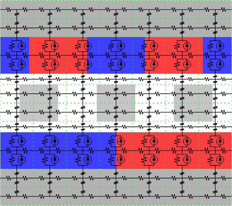
Fig. 8. Example 2D MEC schematic overlay on unrolled radial flux magnetic (where i ≠ j) in PRL(k:k), contains the negative value of the
gear geometry.
equivalent permeance directly connecting the node at the
intersection of the kth radial layer and the ith angular layer and
Each node in the MEC corresponds to a node MMF
the node at the intersection of the kth radial layer and the jth
equation of the same basic form as the one shown in (12), and
angular layer. Because all permeances in the MEC are
there are N2D total nodes in a 2D MEC model, where N2D is the
bidirectional, each matrix PRL(k:k) is symmetric.
product of the number of angular layers, NAL, and the total
number of radial layers, NRL. Thus, the resulting system of
© 2017 IEEE6
P( k :k ),(1:1) - P( k :k ),(1:2) 0 0 - P( k:k),(1:N AL )
- P( k :k ),( 2:1) P( k :k ),( 2:2) - P( k :k ),( 2:3) 0 0
0 - P( k :k ),(3:2)
PRL( k :k ) = (14)
0 0
0 - P( k :k ),( N AL −1:N AL )
- P( k :k ),( N AL:1) 0 0 - P( k :k ),( N AL:N AL −1) P( k :k ),( N AL:N AL )
P( k :k −1),(1:1) 0 0
0 P( k :k −1),( 2:2)
PRL( k :k −1) = PRL( k −1:k ) = (15)
0
0 0 P( k :k −1),( N AL :N AL )
PRL(1:1) - PRL(1:2) 0 0
- PRL( 2:1) PRL( 2:2) - PRL( 2:3)
P2D = 0 - PRL(3:2) 0 (16)
- PRL( N RL −1:N RL )
0 0 - PRL( N RL :N RL −1) PRL( N RL :N RL )
The (NAL x NAL) matrix PRL(k:k-1) defined in (15) contains the the total number of non-zero entries in P2D, is given by
permeances corresponding to paths directly connecting nodes
N NZ2D = N AL (5N RL − 2) (17)
in the kth radial layer to adjacent nodes in radial layer k-1.
Each diagonal entry P(k:k-1),(i:i) in PRL(k:k-1) contains the and the sparsity of P2D can be calculated according to
equivalent permeance directly connecting the ith node in the kth
radial layer to the ith node in radial layer k-1. All other entries N
Sparsity of P2D = 1 − NZ2D 100% . (18)
in PRL(k:k-1) are zero. Because all permeances in the MEC are 2
N 2D
bidirectional, the matrix PRL(k-1:k) is always equal to PRL(k:k-1).
P2D, is then constructed from these constituent submatrices, as Consequently, permeance matrices resulting from MEC
models with reasonable mesh resolutions are extremely sparse;
shown in (16). Thus, the matrix P2D is always symmetric.
therefore, the MATLAB implementation of the MEC model
Each node in the 2D MEC has four adjacent nodes: one on
stores P2D as a sparse matrix in order to dramatically reduce
each of the radial inside, the radial outside, the clockwise
the amount of memory used by the program. For example, for
circumferential side, and the counterclockwise circumferential
side. The only exceptions are the nodes in the innermost and each of the three base designs used in Part II, P2D has a
outermost radial layers, which do not have any adjacent nodes sparsity of at least 99.96% for both the fine and coarse mesh
on the radial inside and radial outside, respectively. settings.
Consequently, each row in P2D corresponding to a node in the
IV. SOLVING THE SYSTEM
first or last radial layers has four non-zero entries, and all
other rows have five non-zero entries, one for each adjacent The 2D MEC model is solved by solving the linear system
node, as well as the diagonal entry in each row. Thus, NNZ2D, of equations given in (13) for the N2D unknown node MMFs in
© 2017 IEEE7
the column vector F2D. If the 2D MEC model has symmetry, where rHS and rLS represent the radii of the integration
then it can be analyzed by solving only the subset of equations (summation) paths in the high and low speed air gaps, while
corresponding to nodes in a symmetrical fraction of the model. Br(r,i) and Bθ(r,i) represent the radial and tangential
Because MMF values represent scalar potentials with respect components of the magnetic flux density in the ith angular
to a reference node, in full 2D MEC models or fractional layer at the specified radius. This study uses integration paths
models with even symmetry, the first node is defined as the corresponding to the radial middle of node cells in the middle
zero potential reference for the rest of the system. This allows layer of each air gap. The flux densities are linearly
the first row of P2D and Φ2D and the first column of P2D to be interpolated with respect to radius and are assumed to be
eliminated, and the remaining system can be solved. invariant with respect to angle within a flux tube. The torque
However, for models with odd symmetry, it is desirable for on the entire modulator structure, τMods, is then given by
corresponding nodes in adjacent fractions of the model to have Mods = −( HSR + LSR ) . (21)
potentials with the same magnitudes and opposite signs. This
choice effectively determines the zero potential reference, V. CONCLUSIONS
which may not correspond to any of the nodes. Thus, for
This is the first part of a two part paper on the development
models with odd symmetry, the first row of P2D and Φ2D and
of a radial flux magnetic gear MEC model. This part presents
the first column of P2D must not be eliminated. the systematic implementation of the MEC model, while Part
In theory, the solution to the system can be obtained by II provides a thorough evaluation and validation of the
inverting the relevant portion of the permeance matrix, based model’s accuracy by comparing its torque and flux density
on the application of the preceding discussion of symmetry predictions against those produced by a commercial non-linear
and the reference node. However, most practical MEC models FEA model. The MEC model is constructed by dividing the
with adequate mesh resolution result in system permeance magnetic gear into radial and angular layers. The number of
matrices which would require a relatively significant amount radial layers in each of the magnetic gear’s 7 different radial
of time and memory to invert; therefore, this implementation regions and the number of angular layers are all independently
solves the MEC system by factorizing the matrix and solving controlled by 8 user specified resolution parameters. Each
the corresponding triangular systems as described in [35]. annular sector defined by the intersection of a radial layer and
This approach dramatically decreases the amount of memory an angular layer corresponds to a node cell, which is the basic
and simulation time required to solve an MEC model. To building block of the MEC. The center of each node cell is a
evaluate the design at different rotor positions, it is necessary node in the magnetic equivalent circuit. Every node cell also
to repeat this process with an adjusted permeance matrix and contains two radially directed reluctances and two tangentially
injected flux vector. However, if the recoil permeability of the directed reluctances, which connect the node to the cell’s
magnets is approximated as the permeability of free space (or boundaries. The reluctances in any one node cell connect to
if the magnets have a 100% tangential fill factor) and the reluctances in neighboring cells and link all of the nodes
modulators are used as the reference frame, only the injected together to form the MEC system network.
flux vector must be adjusted. This can result in significant The (N2D x N2D) MEC system permeance matrix defined in
time savings because the permeance matrix only needs to be (16) contains one row and one column for each node in the
factorized once per design, regardless of the rotor orientations. network. This matrix defines the relationship between each of
Once an MEC model has been solved for the vector of node the N2D node MMFs in the MEC, as described by the system
MMFs, this information can be used along with the matrix equation given in (13), and it is formed based on the
reluctances of the flux tubes to calculate various other user specified discretization settings, magnetic gear
quantities of interest, such as the flux in any flux tube and the geometrical design parameters, and material properties.
flux density at any position in the gear. Due to their coarse Because the system permeance matrix is constructed using
flux tube distributions, many of the other MEC models user specified fixed permeabilities for the different materials,
described in the literature, including most of the few previous the MEC model and system of equations are linear. Once the
magnetic gear MEC studies [28]-[30], [32], use the virtual permeance matrix is constructed, it is factorized to solve the
work (coenergy) method to calculate torque. However, this system of equations and calculate the MMF of each node in
implementation uses Maxwell stress tensors for torque the MEC. This particular implementation capitalizes on any
calculations from the more detailed solutions provided by its symmetry in the gear geometry, as well as the symmetry and
higher resolution flux tube distributions. In particular, the sparsity of the permeance matrix to accelerate the solution
torque on the HSR, τHSR, and the torque on the LSR, τLSR, are process and reduce its memory requirements. The node
calculated using Maxwell stress tensors according to MMFs can then be used along with the discrete MEC
permeances to solve for flux densities and other quantities of
r2 2
Br (rHS , i )B (rHS , i )
N AL
HSR = HS (19) interest, such as the torques on the different gear subsystem
N i =1
0 AL bodies. This systematic implementation of a linear MEC
model allows for extremely fast and accurate analysis of a
r2 2 wide range of practical magnetic gear designs, as
Br (rLS , i )B (rLS , i ) .
N AL
LSR = − LS (20)
N i =1 demonstrated by the various results provided in Part II.
0 AL
© 2017 IEEE8
VI. REFERENCES [25] M. Amrhein and P. T. Krein, "Magnetic Equivalent Circuit Modeling of
Induction Machines Design-Oriented Approach with Extension to 3-D,"
[1] K. Atallah and D. Howe, "A Novel High-Performance Magnetic Gear," in Proc. IEEE Int. Elect. Mach. and Drives Conf., 2007, pp. 1557-1563.
IEEE Trans. Magn., vol. 37, no. 4, pp. 2844-2846, Jul. 2001. [26] M. Amrhein and P. T. Krein, "3-D Magnetic Equivalent Circuit
[2] N. W. Frank and H. A. Toliyat, "Analysis of the Concentric Planetary Framework for Modeling Electromechanical Devices," IEEE Trans.
Magnetic Gear with Strengthened Stator and Interior Permanent Magnet Energy Convers., vol. 24, no. 2, pp. 397-405, Jun. 2009.
Inner Rotor," IEEE Trans. Ind. Appl., vol. 47, no. 4, pp. 1652-1660, Jul.- [27] M. Amrhein and P. T. Krein, "Force Calculation in 3-D Magnetic
Aug. 2011. Equivalent Circuit Networks with a Maxwell Stress Tensor," IEEE
[3] P. O. Rasmussen, T. O. Andersen, F. T. Jorgensen, and O. Nielsen, Trans. Energy Convers., vol. 24, no. 3, pp. 587-593, Sept. 2009.
"Development of a High-Performance Magnetic Gear," IEEE Trans. Ind. [28] M. Fukuoka, K. Nakamura, and O. Ichinokura, "Dynamic Analysis of
Appl., vol. 41, no. 3, pp. 764-770, May-Jun. 2005. Planetary-Type Magnetic Gear Based on Reluctance Network Analysis,"
[4] P. M. Tlali, R.-J. Wang, and S. Gerber, "Magnetic Gear Technologies: A IEEE Trans. Magn., vol. 47, no. 10, pp. 2414-2417, Oct. 2011.
Review," in Proc. Int. Conf. Elect. Mach., 2014, pp. 544-550. [29] M. Fukuoka, K. Nakamura, and O. Ichinokura, "A Method for
[5] M. Johnson, M. C. Gardner, and H. A. Toliyat, "Design and Analysis of Optimizing the Design of SPM Type Magnetic Gear Based on
an Axial Flux Magnetically Geared Generator," IEEE Trans. Ind. Appl., Reluctance Network Analysis," in Proc. Int. Conf. Elect. Mach., 2012,
vol. 53, no. 1, pp. 97-105, Jan.-Feb. 2017. pp. 30-35.
[6] T. V. Frandsen, L. Mathe, N. I. Berg, R. K. Holm, T. N. Matzen, P. O. [30] D. Thyroff, S. Meier, and I. Hahn, "Modeling Integrated Magnetic Gears
Rasmussen, and K. K. Jensen, "Motor Integrated Permanent Magnet Using a Magnetic Equivalent Circuit," in Proc. Annu. Conf. IEEE Ind.
Gear in a Battery Electrical Vehicle," IEEE Trans. Ind. Appl., vol. 51, Electron. Soc., 2015, pp. 2904-2908.
no. 2, pp. 1516-1525, Mar.-Apr. 2015. [31] R. Benlamine, T. Hamiti, F. Vangraefschepe, F. Dubas, and D.
[7] N. W. Frank and H. A. Toliyat, "Gearing Ratios of a Magnetic Gear for Lhotellier, "Modeling of a Coaxial Magnetic Gear Equipped with
Wind Turbines," in Proc. IEEE Int. Elect. Mach. and Drives Conf., Surface Mounted PMs Using Nonlinear Adaptive Magnetic Equivalent
2009, pp. 1224-1230. Circuits," in Proc. Int. Conf. Elect. Mach., 2016, pp. 1888-1894.
[8] K. K. Uppalapati, J. Z. Bird, D. Jia, J. Garner, and A. Zhou, [32] R. C. Holehouse, K. Atallah, and J. Wang, "A Linear Magnetic Gear," in
"Performance of a Magnetic Gear Using Ferrite Magnets for Low Speed Proc. Int. Conf. Elect. Mach., 2012, pp. 563-569.
Ocean Power Generation," in Proc. IEEE Energy Convers. Congr. and [33] M. F. Hsieh and Y. C. Hsu, "A Generalized Magnetic Circuit Modeling
Expo., 2012, pp. 3348-3355. Approach for Design of Surface Permanent-Magnet Machines," IEEE
[9] N. W. Frank and H. A. Toliyat, "Gearing Ratios of a Magnetic Gear for Trans. Ind. Electron., vol. 59, no. 2, pp. 779-792, Feb. 2012.
Marine Applications," in Proc. IEEE Electr. Ship Technol. Symp., 2009, [34] H. W. Derbas, J. M. Williams, A. C. Koenig, and S. D. Pekarek, "A
pp. 477-481. Comparison of Nodal- and Mesh-Based Magnetic Equivalent Circuit
[10] E. Gouda, S. Mezani, L. Baghli, and A. Rezzoug, "Comparative Study Models," IEEE Trans. Energy Convers., vol. 24, no. 2, pp. 388-396, Jun.
between Mechanical and Magnetic Planetary Gears," IEEE Trans. 2009.
Magn., vol. 47, no. 2, pp. 439-450, Feb. 2011. [35] T. A. Davis, "Algorithm 930: FACTORIZE: An Object-Oriented Linear
[11] M. Johnson, M. C. Gardner, and H. A. Toliyat, "Design Comparison of System Solver for MATLAB," ACM Trans. Math. Softw., vol. 39, no. 4,
NdFeB and Ferrite Radial Flux Magnetic Gears," in Proc. IEEE Energy pp. 1-18, Jul. 2013.
Convers. Congr. and Expo., 2016, pp. 1-8.
[12] J. F. H. Douglas, "The Reluctance of Some Irregular Magnetic Fields,"
Trans. AIEE, vol. XXXIV, no. 1, pp. 1067-1134, Apr. 1915. VII. BIOGRAPHIES
[13] E. R. Lwithwaite, "Magnetic Equivalent Circuits for Electrical
Machines," Proc. Inst. Electr. Eng., vol. 114, no. 11, pp. 1805-1809, Matthew Johnson (S’ 13, M’17) earned his B.S. in
Nov. 1967. electrical engineering with a minor in mathematics
[14] C. J. Carpenter, "Magnetic Equivalent Circuits," Proc. Inst. Electr. Eng., from Texas A&M University, College Station, Texas
vol. 115, no. 10, pp. 1503-1511, Oct. 1968. in 2011. In 2017, he received a Ph.D. in electrical
[15] V. Ostovic, "A Method for Evaluation of Transient and Steady State engineering while working in the Advanced Electric
Performance in Saturated Squirrel Cage Induction Machines," IEEE Machines and Power Electronics Laboratory at Texas
Trans. Energy Convers., vol. EC-1, no. 3, pp. 190-197, Sept. 1986. A&M University. His research interests include
[16] V. Ostovic, "Computation of Saturated Permanent-Magnet AC Motor magnetic gears, magnetically geared machines, and
Performance by Means of Magnetic Circuits," IEEE Trans. Ind. Appl., motor drives.
vol. IA-23, no. 5, pp. 836-841, Sept. 1987.
[17] V. Ostovic, "A Novel Method for Evaluation of Transient States in
Saturated Electric Machines," IEEE Trans. Ind. Appl., vol. 25, no. 1, pp. Matthew C. Gardner (S’ 15) earned his B.S. in
96-100, Jan.-Feb. 1989. electrical engineering with a minor in Computer
[18] C. B. Rasmussen and E. Ritchie, "A Magnetic Equivalent Circuit Science from Baylor University, Waco, Texas in
Approach for Predicting PM Motor Performance," in Conf. Rec. IEEE 2014. He is currently pursuing a Ph.D. in electrical
Ind. Appl. Soc. Annu. Meeting, 1997, pp. 10-17 vol.1. engineering while working in the Advanced Electric
[19] J. Perho, "Reluctance Network for Analysing Induction Machines," Machines and Power Electronics Laboratory at Texas
Ph.D. dissertation, Dept. Elect. and Commun. Eng., Helsinki Univ. A&M University. His research interests include
Tech., Espoo, Finland, 2002. optimal design and control of magnetic gears and
[20] S. D. Sudhoff, B. T. Kuhn, K. A. Corzine, and B. T. Branecky, magnetically geared machines.
"Magnetic Equivalent Circuit Modeling of Induction Motors," IEEE
Trans. Energy Convers., vol. 22, no. 2, pp. 259-270, Jun. 2007.
[21] M. Yilmaz and P. T. Krein, "Capabilities of Finite Element Analysis and
Hamid A. Toliyat (S’87, M’91, SM’96, F’08)
Magnetic Equivalent Circuits for Electrical Machine Analysis and
received the B.S, degree from Sharif University of
Design," in Proc. IEEE Power Electron. Specialists Conf., 2008, pp.
Technology, Tehran, Iran in 1982, the M.S. degree
4027-4033.
from West Virginia University, Morgantown, WV in
[22] M. Amrhein and P. T. Krein, "Magnetic Equivalent Circuit Simulations
1986, and the Ph.D. degree from University of
of Electrical Machines for Design Purposes," in Proc. IEEE Elect. Ship
Wisconsin-Madison, Madison, WI in 1991, all in
Technol. Symp., 2007, pp. 254-260.
electrical engineering. Following receipt of the Ph.D.
[23] M. F. Hsieh and Y. C. Hsu, "A Generalized Magnetic Circuit Modeling
degree, he joined the faculty of Ferdowsi University
Approach for Design of Surface Permanent-Magnet Machines," IEEE
of Mashhad, Mashhad, Iran as an Assistant Professor
Trans. Ind. Electron., vol. 59, no. 2, pp. 779-792, Feb. 2012.
of Electrical Engineering. In March 1994 he joined
[24] C. Bruzzese, D. Zito, and A. Tessarolo, "Finite Reluctance Approach: A
the Department of Electrical and Computer Engineering, Texas A&M
Systematic Method for the Construction of Magnetic Network-Based
University where he is currently the Raytheon endowed professor of electrical
Dynamic Models of Electrical Machines," in Proc. AEIT Annu. Conf.,
engineering. Dr. Toliyat has many papers and awards to his name, including
2014, pp. 1-6.
the Nikola Tesla Field Award.
© 2017 IEEEYou can also read