A rapidly converging initialisation method to simulate the present-day Greenland ice sheet using the GRISLI ice sheet model (version 1.3) ...
←
→
Page content transcription
If your browser does not render page correctly, please read the page content below
Geosci. Model Dev., 12, 2481–2499, 2019
https://doi.org/10.5194/gmd-12-2481-2019
© Author(s) 2019. This work is distributed under
the Creative Commons Attribution 4.0 License.

A rapidly converging initialisation method to simulate the
present-day Greenland ice sheet using the GRISLI
ice sheet model (version 1.3)
Sébastien Le clec’h1,2 , Aurélien Quiquet1,3 , Sylvie Charbit1 , Christophe Dumas1 , Masa Kageyama1 , and
Catherine Ritz4
1 Laboratoire  des Sciences du Climat et de l’Environnement, LSCE/IPSL, CEA-CNRS-UVSQ,
Université Paris-Saclay, Gif-sur-Yvette, France
2 Earth System Science and Department Geografie, Vrije Universiteit Brussel, Brussels, Belgium
3 Institut Louis Bachelier, Chair Energy and Prosperity, Paris, 75002, France
4 Institut des Géosciences de l’Environnement, Université Grenoble-Alpes, CNRS, 38000 Grenoble, France

Correspondence: Sébastien Le clec’h (sebastien.le.clech@vub.be)

Received: 22 December 2017 – Discussion started: 8 February 2018
Revised: 16 April 2019 – Accepted: 20 April 2019 – Published: 27 June 2019

Abstract. Providing reliable projections of the ice sheet con-        the deformation rates. We show that this factor has a strong
tribution to future sea-level rise has become one of the main         impact on the minimisation of ice thickness errors and has
challenges of the ice sheet modelling community. To increase          to be chosen as a function of the internal thermal state of
confidence in future projections, a good knowledge of the             the ice sheet (e.g. a low enhancement factor for a warm ice
present-day state of ice flow dynamics, which is critically           sheet). While the method performance slightly increases with
dependent on basal conditions, is strongly needed. The main           the duration of the minimisation procedure, an ice thickness
difficulty is tied to the scarcity of observations at the ice–        root mean square error (RMSE) of 50.3 m is obtained in only
bed interface at the scale of the whole ice sheet, resulting in       1320 model years. This highlights a rapid convergence and
poorly constrained parameterisations in ice sheet models. To          demonstrates that the method can be used for computation-
circumvent this drawback, inverse modelling approaches can            ally expensive ice sheet models.
be developed to infer initial conditions for ice sheet mod-
els that best reproduce available data. Most often such ap-
proaches allow for a good representation of the mean present-
day state of the ice sheet but are accompanied with unphys-           1   Introduction
ical trends. Here, we present an initialisation method for
the Greenland ice sheet using the thermo-mechanical hybrid            Recent observations provide evidence that the rate of mass
GRISLI (GRenoble Ice Shelf and Land Ice) ice sheet model.             loss of the Greenland ice sheet (GrIS) is continuously in-
Our approach is based on the adjustment of the basal drag co-         creasing (Mouginot et al., 2015; Rignot et al., 2015). Simu-
efficient that relates the sliding velocities at the ice–bed inter-   lating the GrIS response under future warm periods is there-
face to basal shear stress in unfrozen bed areas. This method         fore crucial to establish reliable projections of future sea-
relies on an iterative process in which the basal drag is peri-       level rise at decade to century timescales (Bindschadler et al.,
odically adjusted in such a way that the simulated ice thick-         2013; Edwards et al., 2014) but also to investigate the effects
ness matches the observed one. The quality of the method              of ice sheet changes on the climate system (Swingedouw
is assessed by computing the root mean square errors in ice           et al., 2013; Böning et al., 2016; Hansen et al., 2016; De-
thickness changes. Because the method is based on an adjust-          france et al., 2017). As a result, better constraining the GrIS
ment of the sliding velocities only, the results are discussed        evolution has become a key objective of the climate and ice
in terms of varying ice flow enhancement factors that control         sheet modelling communities.

Published by Copernicus Publications on behalf of the European Geosciences Union.
2482                                S. Le clec’h et al.: A rapidly converging Greenland ice sheet model initialisation method

   Reliable simulations of the GrIS require a proper ice sheet           A second category of initialisation methods relies on data
model initialisation procedure to avoid an unphysical model           assimilation techniques, whose goal is to infer model param-
drift which can be caused by inconsistencies between the ini-         eters or poorly known boundary conditions and which are
tial conditions of the ice sheet model and the boundary condi-        also used to minimise the mismatch between model vari-
tions (external forcing fields). These initialisation procedures      ables (most often surface velocities) and observations (e.g.
consist of finding the initial physical state of the ice sheet        Arthern and Gudmundsson, 2010; Gillet-Chaulet et al., 2012;
(such as the internal temperature), the model parameters and          Morlighem et al., 2010). However, this approach may lead to
sometimes the boundary conditions that best reproduce the             internal inconsistencies between the simulated internal con-
observations with a minimal model drift. Recent observa-              ditions (temperature and velocities) or between the simu-
tions, such as surface and bedrock topographies (Bamber               lated ice velocities and the observational datasets, such as
et al., 2013) and horizontal surface velocity (Joughin et al.,        surface and bedrock topography. These inconsistencies may
2018) offer only a partial description of the GrIS current state      have a strong impact on the results of forward simulations. To
and a major source of uncertainty lies in the poor knowledge          circumvent this drawback, other authors (e.g. Perego et al.,
of the basal properties (e.g. water content in the sediment or        2014; Mosbeux et al., 2016) developed a multi-parameter in-
basal dragging) and of the internal thermo-mechanical con-            version technique to optimise both the sliding velocities and
ditions (e.g. temperature and deformation profile). Indeed,           the bedrock topography in such a way that the modelled sur-
both the basal properties and the internal conditions have a          face ice velocities match with the observed ones. This allows
strong impact on the ice motion and thus on the simulated             the set of initial conditions to be self-consistent. However,
GrIS state (Weertman, 1957; Boulton and Hindmarsh, 1987;              if not constrained by observed ice thickness, these methods
Kulessa et al., 2017). Optimising the initialisation procedure        may lead to unrealistic simulated topography. An alternative
of ice sheet models is therefore an active area of research           approach, which avoids the previously mentioned shortcom-
and a multidisciplinary effort. The ice sheet model initialisa-       ings, consists of considering only the observed ice sheet ge-
tion experiments intercomparison project (initMIP) (Goelzer           ometry as the final target by finding appropriate basal con-
et al., 2018) gives a recent example of this effort. Its goal is to   ditions (generally the basal drag coefficient; see Sect. 2) that
compare different initialisation techniques and to assess their       minimise the differences between observed and simulated ice
impact on the dynamic responses of the models.                        thickness (Pollard and DeConto, 2012; Pattyn, 2017). How-
   The goal of ice sheet model initialisation is to infer inter-      ever, methods that choose to invert the basal drag coefficient
nal properties (e.g. temperature), some boundary conditions           only are not able to correct ice thickness errors in regions
(e.g. basal drag) and model parameter values. To this aim,            where there is no sliding (i.e. where the bed is frozen). More-
different techniques have been developed. One approach is to          over, while inverse methods are designed to produce an ice
allow the ice sheet model to evolve freely over a long enough         sheet state close to observations, the inferred basal drag co-
time (ice sheet spin-up). This approach has long been the             efficient may cancel errors coming from erroneous simulated
most commonly used technique to initialise ice sheet models           basal temperatures and/or model physics shortcomings. Yet,
(Huybrechts and de Wolde, 1999; Huybrechts et al., 2002;              as outlined by Pollard and DeConto (2012), the risk of can-
Charbit et al., 2007, and other references in Rogozhina et al.,       celling errors is of less importance compared to those related
2011). It consists of simulating the ice sheet during one or          to inconsistencies between internal conditions and surface
more glacial–interglacial cycles to account for the long-term         properties that will likely to be considerably reduced with
ice sheet history and thereby to obtain internal consistency          expected future improvements in ice sheet models and better
between the simulated ice sheet and the climate forcing evo-          observations of basal conditions.
lution derived from ice core records. Even if model parame-              Here, we present a new iterative initialisation procedure
ters can be chosen to reduce the mismatch between modelled            that relies on the same basic principles as those developed
and observed present-day ice sheet state (e.g. topography, ve-        by Pollard and DeConto (2012) (referred to as PDC12 in
locity), this approach may lead to important errors. In addi-         the following) and applied by Pattyn (2017) for the Antarc-
tion, due to the long integrations needed ( > 10 000–100 000-         tic ice sheet using linear and non-linear sliding laws. Simi-
year long), such spin-up methods can only be used with low            larly to PDC12, we compute the basal drag coefficient that
computational-cost models, which are often unable to prop-            minimises the error in the simulated ice thickness and relates
erly capture fast ice flow processes. To compute the internal         basal stresses to basal velocities. However, while PDC12 re-
properties, an alternative approach is to keep the topography         quires long (multi-millennial) integrations for the method to
fixed, while vertical temperature fields, and possibly veloc-         converge, we suggest instead an iterative method of short
ity fields, are allowed to freely evolve (e.g. Sato and Greve,        (decadal to centennial) integrations starting from the ob-
2012; Seddik et al., 2012). In this case, because the simulated       served ice thickness. Our iterative method ensures a more
ice flux divergence is generally far from being balanced by           rapid convergence and is thus suitable for computationally
the net mass balance (i.e. surface and basal mass balance),           expensive models.
an artificial drift arises when free evolving topography is re-          The paper is organised as follows. In Sect. 2 we present the
stored (Goelzer et al., 2017).                                        main characteristics of the ice sheet model used in this study.

Geosci. Model Dev., 12, 2481–2499, 2019                                                 www.geosci-model-dev.net/12/2481/2019/
S. Le clec’h et al.: A rapidly converging Greenland ice sheet model initialisation method                                      2483

Section 3 describes the iterative minimisation procedure in            To describe the effect of ice rheology, the deformation
detail. The main results are presented in Sect. 4 and sensi-        rate and stresses are related via Glen’s flow law (Glen et al.,
tivity experiments in Sect. 5. These sections are followed by       1957). As in other large-scale ice sheet models, GRISLI uses
a discussion and the main conclusions of the present study          a flow enhancement factor (Ef) in Glen’s flow law to artifi-
(Sect. 6).                                                          cially account for the impact of ice anisotropy on the defor-
                                                                    mation rate. This enhancement factor depends on the stress
                                                                    regime (e.g. Huybrechts, 1990). Lower enhancement factors
2   The ice sheet model GRISLI                                      lead to lower deformation rates and as such to slower ice ve-
                                                                    locities. The grounding line position is defined according to
The GRISLI (GRenoble Ice Shelf and Land Ice) ice sheet              a flotation criterion and floating points are treated following
model was first designed to describe the Antarctic ice sheet        the SSA only. Calving physics is not explicitly computed,
(Ritz et al., 2001) and further adapted to the Northern Hemi-       but if a grid point at the ice-shelf front fails at maintaining a
sphere ice sheets (Peyaud et al., 2007). The version used           thickness threshold, it is automatically calved (Peyaud et al.,
in this study has been specifically developed for Green-            2007). The ice thickness cut-off threshold is set to 250 m.
land (Quiquet et al., 2012) with a horizontal resolution of            Since GRISLI is thermo-mechanically coupled, the ice
5 km ×5 km (301 × 561 grid points) and 21 evenly spaced             temperature influences the ice velocity via the viscosity. The
vertical levels. GRISLI accounts for the coupled behaviour of       temperature is computed both in the ice and in the bedrock
temperature and velocity fields. It relies on basic principles of   by solving a time-dependent heat equation. The temperature
mass, heat and momentum conservation. The evolution of ice          signal itself depends on ice deformation, surface temperature
sheet geometry is a function of surface mass balance, ice dy-       forcing and geothermal heat flux.
namics and bedrock altitude. Since this study only deals with
present-day steady-state simulations, the module describing
the isostatic adjustment is not activated here. The evolution
                                                                    3   Iterative minimisation procedure
of the ice thickness is governed by the mass balance equa-
tion:                                                               The basic principle of inverse modelling approaches for the
∂H                                                                  ice sheet initialisation procedure is to adjust the basal drag
    = −∇(U G H ) + SMB − bmelt ,                             (1)    coefficient (β) which varies spatially, in order to reduce the
 ∂t
                                                                    mismatch between the simulated surface ice velocities and/or
where H is the ice thickness, U G is the depth-averaged ve-         the ice sheet geometry and the observed ones.
locity (2-D vector), SMB is the surface mass balance and               While numerous studies are based on fitting the modelled
bmelt is the basal melting.                                         ice velocities (e.g. Gudmundsson and Raymond, 2008; Arth-
   The ice flow velocity is derived from a simplified formu-        ern and Gudmundsson, 2010; Morlighem et al., 2010; Gillet-
lation of the Stokes equations (i.e. the stress balance) using      Chaulet et al., 2012; Perego et al., 2014) or both surface ve-
the shallow-ice (Hutter, 1983) and shallow-shelf (MacAyeal,         locities and basal topography (Perego et al., 2014; Mosbeux
1989) approximations. The shallow-ice approximation (SIA)           et al., 2016), only few authors have opted for fitting ice sur-
assumes that, owing to the small ratio of vertical to horizon-      face elevation (Pollard and DeConto, 2012; Pattyn, 2017).
tal dimensions of the ice sheet, longitudinal stresses can be       Here, we decided to adjust the basal sliding velocities via the
neglected with respect to vertical shearing along the steepest      adjustment of the β coefficient to fit the GrIS thickness to the
slope. Conversely, in the shallow-shelf approximation (SSA),        observed one. Similarly to Perego et al. (2014), our choice is
the horizontal strain rates become dominant and the horizon-        motivated by the need to refine the estimates of GrIS contri-
tal velocities do not vary with depth. In the model, the veloc-     bution to future sea-level rise without the sea-level rise sig-
ities are computed as the heuristic sum of the SSA and the          nal being contaminated by unphysical transients from the ini-
SIA components, as in Bueler and Brown (2009) but with              tial condition. However, while Perego et al. (2014) adopted
a no-weighting function (Winkelmann et al., 2011). In this          a formal minimisation approach (i.e. adjoint-based model),
case, the SSA velocity is used as the sliding velocity. We          we suggest instead an ad hoc method potentially applicable
assume no-slip conditions for a frozen bed (i.e. basal temper-      to any ice sheet model.
ature below the melting point), and in these conditions, the           The GRISLI climate forcing, i.e. surface mass balance and
SSA velocity is set to 0. In the model version used in this         surface air temperature (Fig. 1), is provided by the regional
study, we assume a linear viscous till with a uniform thick-        atmospheric model MAR (Fettweis et al., 2013) forced at its
ness, in which the basal shear stress (τ b ) and basal velocity     boundary by the ERA-Interim reanalyses (Berrisford et al.,
(ub ) are related via the following expression:                     2011). Both forcing fields are averaged over the 1979–2005
                                                                    period (Fig. 1a and b). They are interpolated on the GRISLI
τ b = −βub ,                                                 (2)    grid (5 km ×5 km) and corrected for surface elevation differ-
                                                                    ences between MAR and GRISLI by applying the method
where β is the basal drag coefficient and varies with space.        developed by Franco et al. (2012). For the geothermal heat

www.geosci-model-dev.net/12/2481/2019/                                                Geosci. Model Dev., 12, 2481–2499, 2019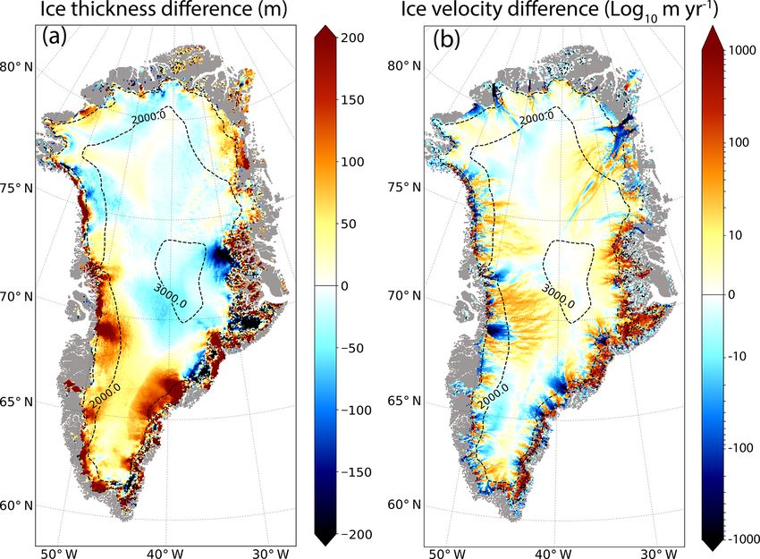
2484                               S. Le clec’h et al.: A rapidly converging Greenland ice sheet model initialisation method

flux we use the data generated for the SeaRISE (Sea-level
Response to Ice Sheet Evolution) project (Fox Maule et al.,
2005). The initial geometry consists of the present-day ob-                              HG
                                                                       U corr = U G ×          .                              (3)
served ice thickness and bedrock elevation taken from Bam-                               H obs
ber et al. (2013). To compute initial conditions consistent
with the boundary conditions, we run a 30 000-year integra-            As seen before (Sect. 2), the mean velocity field U G is
tion of the model imposing a fixed topography. For this long           the sum of two velocity components: the sliding veloc-
experiment, similar to the fixed topography spin-up method,            ity U sli and the vertically averaged velocity U def due to
we assumed a perpetual present-day climate forcing (Fig. 1a            vertical ice deformation:
and b) and we used a basal drag coefficient (Fig. 2a) coming
                                                                       U G = U sli + U def .                                  (4)
from a previous simulation carried out within the Ice2Sea
project (Edwards et al., 2014). The resulting basal tempera-
                                                                       Assuming that the differences between U G , the simu-
ture after this long integration, presented as a difference with
                                                                       lated vertically averaged velocity field, and U corr , the
respect to the pressure melting point, is shown in Fig. 1c.
                                                                       idealised vertically averaged velocity field, are only due
It shows areas with temperature largely below the pressure
                                                                       to changes in the sliding velocity U sli , we can write
melting point, associated with frozen bed, and areas with
temperature at the pressure melting point (red colours), as-
                                                                       U corr = U sli     def
                                                                                  corr + U .                                  (5)
sociated with thawed bed. Compared to the recent synthe-
sis of GrIS basal temperatures (see Fig. 11 in MacGregor               Following Eqs. (4) and (5), we can deduce the corrected
et al., 2016), our initial basal temperature generally agrees          sliding velocity (U sli
                                                                                           corr ):
well with the reconstructions in the north-western and north-
eastern parts of the GrIS but is probably overestimated, with          U sli              G   sli
                                                                         corr = U corr − U + U .                              (6)
too large a thawed bed area, in the eastern and central parts
of the GrIS (not shown). The impact of ice temperature on              U sli
                                                                         corr represents the corrected sliding velocity whose
the minimisation procedure is discussed in Sect. 5.1.                  difference with U sli indicates how the simulated sliding
   In order to avoid inconsistencies between the different             velocity must change to reduce the mismatch between
datasets used as boundary and initial conditions, GRISLI is            H G and H obs .
first run forward (free-evolving surface elevation and temper-
                                                                       As such, we use the ratio between
                                                                                                     sli the
                                                                                                           simulated and the
ature) for 5 years (relaxation step, blue box in Fig. 3). After
this short relaxation period, we start the iterative minimisa-         corrected sliding velocities Usli to compute a new
                                                                                                       U corr
tion procedure (red box in Fig. 3). This procedure is based            basal drag coefficient (β new ). This results in slowing
on an iterative process set up to adjust the basal drag coeffi-        down or speeding up the simulated sliding velocity and
cient in such a way that the mismatch between observed and             acts to reduce the gap between H G and H obs :
simulated ice thickness is reduced. Instead of optimising the
basal drag coefficient every 5000 years as in PDC12, here the                            U sli
                                                                       β new = β old ×            .                           (7)
optimisation is done at every time step (which is set to 1 year                          U sli
                                                                                           corr
for the present study), using an ice thickness ratio to correct
the simulated sliding velocity with the help of a modification         Equation (7) is essentially identical to what is done
of the basal drag coefficient.                                         in Price et al. (2011) except that they use observed
   The iterative minimisation procedure itself consists of re-         and modelled velocities rather than observed and mod-
peated cycles, each cycle being divided into two main steps            elled ice thickness to adjust the basal drag coefficient.
(red box in Fig. 3):                                                   It should be noted that U sli
                                                                                                   corr can be lower or equal
                                                                       to 0, leading to infinite or negative basal drag coeffi-
first step: The first step consists of a free-evolving simula-         cient. This can happen when the velocity due to verti-
      tion (thickness and temperature) during which we ad-             cal shearing U def is greater or equal to U corr . In this
      just, at each model time step, the basal drag coefficient        case we artificially impose a no-slip condition by as-
      so that the ice thickness difference with respect to the         signing to the basal drag coefficient a maximum value
      observations becomes minimal. To this end, from the              set to 5×10⁵ Pa yr m−1 . On the other hand, in case of too
      simulated vertically averaged velocity (U G ) computed           small a U def velocity, β may be as low as 1 Pa yr m−1 to
      from the previous time step (or from the values obtained         facilitate ice sliding. Owing to its design, the method
      after the relaxation for the first iteration), we compute a      is only able to correct for the ice thickness mismatch
      corrected vertically averaged velocity field (U corr ) as a      where sliding occurs, i.e. where the base of the ice sheet
      function of the computed (H G ) and observed ice thick-          is at the pressure melting point. Throughout this step,
      ness (H obs ):                                                   the basal drag coefficient is updated at each time step
                                                                       for each model grid point. In the following, the duration

Geosci. Model Dev., 12, 2481–2499, 2019                                             www.geosci-model-dev.net/12/2481/2019/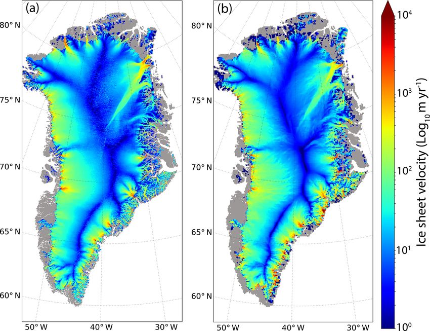
S. Le clec’h et al.: A rapidly converging Greenland ice sheet model initialisation method                                                 2485

Figure 1. (a, b) Climate forcing averaged over the 1979–2005 period simulated by the atmospheric regional model MAR (Fettweis et al.,
2013) and interpolated on the GRISLI ice sheet model grid (5 km ×5 km): mean surface mass balance (m yr−1 , i.e. 103 kg m−2 yr−1 ) with
the black line representing the equilibrium line altitude, defined as the frontier between accumulation and ablation areas; mean annual surface
temperature (◦ C) with the white dashed lines representing the 5 ◦ C iso-contours. In addition, (c) basal temperature difference with respect to
the pressure melting point (◦ C) at the end of the 30 000-year equilibrium temperature computation for a fixed topography.

Figure 2. Spatial distribution of the basal drag coefficient (log10 Pa yr m−1 ) in (a) the initial condition, used in the GRISLI Ice2Sea simula-
tions; (b) the iterative cycle that produces the minimal RMSE (Nbcycle = 9) when using Ef = 1 for Nbinv = 20 years and Nbfree = 200 years
(Sect. 4.2); (c) the iterative cycle that produces the minimal RMSE (Nbcycle = 9) when using Ef = 1 for Nbinv = 20 years and Nbfree =
200 years but starting from a uniform basal drag coefficient (Sect. 5.2).

     of this step is referred to as Nbinv and has a typical value               As such, the adjustment of the basal drag coefficient is
     of a few decades.                                                          stronger in regions dominated by ice deformation.

     Note that, using Eqs. (3) and (4), we can show that                  second step: The second step consists of running a new
     Eq. (7) can be rewritten as                                              free-evolving simulation but this time using a time-
                                                                              constant (but spatially varying) basal drag coefficient,
      β old       U def                   HG                                  i.e. the last inferred basal drag coefficient of the first
            = rH + sli (rH − 1) where rH = obs .                 (8)          step. The duration of this second step, referred to as
      β new       U                       H

www.geosci-model-dev.net/12/2481/2019/                                                         Geosci. Model Dev., 12, 2481–2499, 2019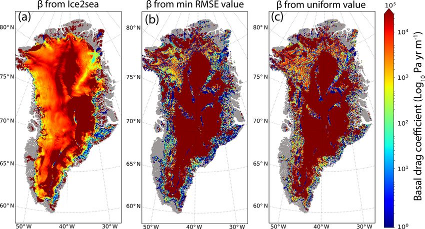
2486                                S. Le clec’h et al.: A rapidly converging Greenland ice sheet model initialisation method

                                                                       mate the balance velocity, that is the depth-averaged velocity
                                                                       required to maintain the steady-state of the ice sheet.
                                                                          Once the optimal basal drag coefficient is found, it can
                                                                       be used to run prognostic forward simulations such as in Le
                                                                       clec’h et al. (2019) and Goelzer et al. (2018).

Figure 3. Schematic representation of the iterative minimisation       4     Results
procedure method. The iterative process itself (steps 1 and 2) is
shown in the red box. The assessment of the performance of the         4.1    The importance of the initialisation procedure
method for a given cycle (e.g. RMSE and trend discussed in Sects. 4
and 5) is performed at 200 years of the second step (green box), in-   To illustrate the need for an initialisation procedure, we per-
dependently of the value of Nbfree . The initial conditions for the    formed a 200-year long free-evolving simulation without any
iterations are the results of the 30 000-year temperature computa-     specific initialisation procedure using the mean 1979–2005
tion using a fixed topography (black box) followed by a relaxation     climatic forcing presented in Sect. 3. For this simulation, the
of the surface topography (blue box).                                  initial internal condition corresponds to the one obtained af-
                                                                       ter the 30 000-year temperature equilibrium simulations (see
                                                                       Sect. 3), and the basal drag coefficient, coming from previous
       Nbfree in the following, is generally longer than that of
                                                                       Ice2Sea simulations (Edwards et al., 2014), is left unchanged
       the first step, typically a few decades to a few centuries.
                                                                       (Fig. 2a).
       This step aims to quantify the model drift and the model
                                                                          The simulated GrIS volume obtained for this experiment
       mismatch with observations for the inferred basal drag
                                                                       is 1.4 % higher than the one estimated by Bamber et al.
       coefficient. The simulated ice sheet velocity and topog-
                                                                       (2013) from observations (2.71 × 10⁶ Gt). This overestima-
       raphy at the end of this second step are used to compute
                                                                       tion is driven by large positive ice thickness differences
       a new U corr value in order to start a new cycle from the
                                                                       (> 200 m) with respect to observations in the margin regions
       first step. The number of iterative cycles will be noted
                                                                       (Fig. 4a). There are also negative ice thickness differences in
       Nbcycle in the following.
                                                                       the interior of the ice sheet, in particular in the central east-
     In summary, our iterative minimisation procedure consists         ern region. On top of this geometry mismatch, this experi-
of                                                                     ment also presents a drift at the end of the 200 years with
                                                                       a negative contribution to global sea level of 0.7 mm yr−1
     i. adjustment of the basal drag coefficient at each time step     (i.e. 263 Gt yr−1 ice mass gain). Compared to observations
        (each year) for Nbinv years (first step, Eqs. 3 to 7).         (Joughin et al., 2018), the simulated ice velocity presents the
                                                                       same large-scale pattern but with important local differences
 ii. free-evolving simulation with the last inferred basal             (Fig. 4b). In particular, the main GrIS glaciers are generally
     drag coefficient from (i) for Nbfree years (second step).         too slow.
                                                                          These results show the limitations of the simulated GrIS
 iii. repeating the steps (i) and (ii) Nbcycle times.                  under constant climate forcing without an appropriate initial-
                                                                       isation procedure. In this specific case, the simulated model
   In addition, to assess the performance of the minimisation          drift can potentially counterbalance the effect of climate
procedure (i.e. the quality of the inferred basal drag coeffi-         warming expected in the future, leading to an unrealistic
cient), we compute some quality metrics at the end of each             projected Greenland melting contribution to global sea-level
cycle (green box in Fig. 3). The metrics are computed at               rise. Therefore, the use of an initialisation procedure to min-
the year 200 of the free-evolving simulation of the second             imise the model drift with a realistic simulated topography
step, independently of its duration (i.e. Nbfree ). If Nbfree is       is not avoidable if the goal is to produce reliable sea-level
shorter than 200 years, we simply extend the simulation for            projections.
200 years. The quality metrics discussed in Sect. 4 include
in particular the root mean square error (RMSE) of the sim-            4.2    Iterative minimisation performance for a range of
ulated ice thickness with respect to the observations and the                 enhancement factor values
drift in geometry (integrated ice thickness changes). These
metrics help to decide whether an additional cycle is required         An increase (a decrease) in the basal drag coefficient (β)
or not. In the following, we also discuss the spatial patterns         slows down (speeds up) the sliding velocity and thus the ice
of ice thickness and ice velocity mismatches with respect to           flow. Based on the adjustment of the sliding velocity, our iter-
observations. Our method does not use the observed surface             ative minimisation procedure allows for a tuning of β only in
velocity as a constraint. However, at the end of the minimi-           regions where the basal temperature is at the pressure melt-
sation procedure (e.g. minimal thickness error and minimal             ing point, i.e. where the ice can slide over the bedrock. Where
drift), the simulated velocity tends nonetheless to approxi-           the base is frozen, the tuning of the basal drag coefficient has

Geosci. Model Dev., 12, 2481–2499, 2019                                                  www.geosci-model-dev.net/12/2481/2019/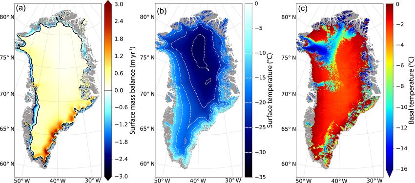
S. Le clec’h et al.: A rapidly converging Greenland ice sheet model initialisation method                                          2487

                                                                        4.2.1   Root mean square error

                                                                        The ice thickness RMSE defined with respect to observations
                                                                        is displayed in Fig. 5 as a function of the number of cycles
                                                                        performed for the different enhancement factors. For a given
                                                                        Ef value, the RMSE quickly decreases during the first cy-
                                                                        cles and generally stabilises after Nbcycle ≈ 5–6. This means
                                                                        that the procedure is very effective in reducing the ice thick-
                                                                        ness error for the first iterations but does not entirely correct
                                                                        the mismatch with observations. Depending on the enhance-
                                                                        ment factor considered, the overall improvement represents
                                                                        a reduction of about 20 to 40 m in ice thickness RMSE with
                                                                        respect to the first iterative cycle.
                                                                           The RMSE is largely different for the different enhance-
                                                                        ment factors. For Ef > 2, we systematically have a larger
                                                                        RMSE for a larger Ef value regardless of the number of
Figure 4. (a) Ice thickness difference (m) simulated at the end of a    iterative cycles performed. This is no longer the case for
200-year-long simulation without any specific initialisation proce-     smaller Ef since the experiment (i.e. the Ef value) providing
dure with respect to the observed ice thickness from Bamber et al.      the lowest RMSE is different for the Nbcycle considered. For
(2013). (b) Difference (m yr−1 ) between the surface ice velocity in
                                                                        Ef = 0.5 the RMSE value is often larger than that obtained
the same simulation and the observed surface velocity from Joughin
et al. (2018). The dashed lines correspond to the 1000 m surface el-
                                                                        with Ef = 2.5 even with increasing Nbcycle . Indeed, Ef = 0.5
evation iso-contours for the simulated topography. Grey areas rep-      implies too small a deformation rate that leads to too slow an
resent non-ice-covered areas. A logarithmic scale is used for the ice   ice flow velocity. The departure from the observations is thus
velocity difference.                                                    mainly characterised by positive ice thickness anomalies at
                                                                        the edges and in the southern half of the ice sheet. The simu-
                                                                        lations with Ef varying from 1 to 2 have very similar RMSE
no impact on the ice thickness minimisation because no slid-            even if 1.5 has a slightly lower RMSE in most cases. While
ing occurs. In order to slow down or speed up the ice flow              the lower RMSE value (49.8 m) is obtained for Ef = 1.5 after
in such regions, the value of the enhancement factor, Ef (see           nine cycles (Table 1), RMSE values below 55 m are obtained
Sect. 2), can be tuned. As explained in Sect. 2, this factor            after four cycles for Ef varying from 1 to 2. Considering that
is used to increase (when > 1) or decrease (when < 1) the               after one cycle the error is greater than 80 m, we are able to
ice deformation velocity. The more the ice deformation is               improve the RMSE by about 30 m in 880 years of simulations
increased (decreased), the more the ice flow in frozen base             (4 × 220 years).
region speed-ups (slow-downs) and thus decrease (increase)
the ice thickness.                                                      4.2.2   Model structural biases and consequence on total
   The enhancement factor for the SIA regime (slow ice flow)                    ice volume
is expected to have a large influence on shear-stress-driven
velocities (Quiquet et al., 2018). Generally set to 3 (Ritz             (a) Where are the errors? Correction by deformation
et al., 2001), the Ef can be chosen within a large range of             and basal sliding
values between 1 and 10 (Ma et al., 2010). In the following,
we assess our iterative minimisation procedure for a range of           In addition to the RMSE criterion, which is an integrated
Ef values: 0.1, 0.5, 1, 1.5, 2, 2.5, 4, 3, 3.5, 4, 4.5 and 5. For       metric, the maps of the difference between the simulated and
this, we use an Nbinv of 20 years and an Nbfree of 200 years            the observed ice thickness bring valuable information to un-
and perform 15 iterative cycles (Nbcycle ). For the first cycle,        derstand the model structural biases. In Fig. 6, we can dis-
i.e. Nbcycle = 1, all the Ef experiments start from the identi-         tinguish two main patterns. Except for Ef = 0.5, all the Ef
cal initial conditions and basal drag coefficient presented in          experiments with an Nbcycle producing the minimum RMSE
Sect. 3.                                                                value (Fig. 6 and Table 1) are marked with an underesti-
   Each of the 180 experiments (15 cycles for 12 enhance-               mation in ice thickness in the interior and an overestima-
ment factors) are evaluated after 200 years of the free-                tion at the edges of the GrIS. This overestimation can be
evolving simulation (second step; see Sect. 3) using 1-D met-           slightly reduced using higher Ef values, but the underesti-
rics (ice thickness RMSE, global ice volume, geometry drift)            mation nonetheless gets larger in this case.
and 2-D validation criteria (ice thickness differences).                   As explained above, larger Ef values amplify ice deforma-
                                                                        tion and therefore speed up the ice velocity, explaining the
                                                                        spread of the regions where the ice thickness is underesti-
                                                                        mated (Fig. 6). Some of these regions, such as a significant

www.geosci-model-dev.net/12/2481/2019/                                                    Geosci. Model Dev., 12, 2481–2499, 2019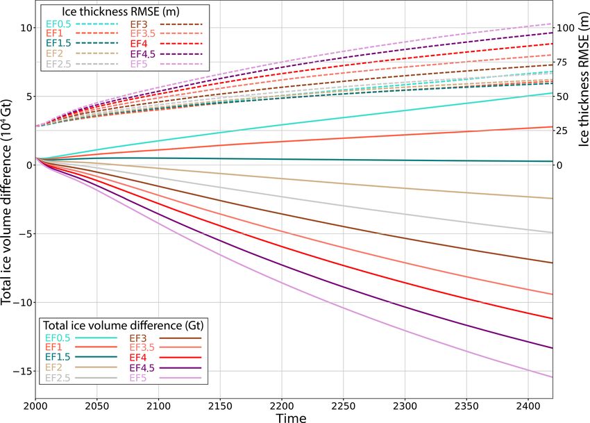
2488                                       S. Le clec’h et al.: A rapidly converging Greenland ice sheet model initialisation method

Figure 5. Ice thickness root mean square error with regard to observations from Bamber et al. (2013), in metres for Nbinv = 20, Nbfree = 200
and with enhancement factors (Ef) ranging from 0.5 to 5 as a function of the number of iterations (Nbcycle ).

Table 1. Integrated metrics computed from the last 5 years of the 200-year free-evolving simulations of the second step (green box in Fig. 3)
for Nbinv = 20 and Nbfree = 200 with varying enhancement factors (Ef) ranging from 0.5 to 5.

         Enhancement factor value           Ef = 0.5   Ef = 1   Ef = 1.5    Ef = 2   Ef = 2.5    Ef = 3   Ef = 3.5    Ef = 4   Ef = 4.5    Ef = 5
                       RMSE (m)                 53.0     50.3      50.8       52.3      55.4       59.3      64.6       70.4      74.8       78.8
  Nbcycle = 6    Volume difference (Gt)       33089    20671       7579     −7224    −22290     −36570    −49727     −64113    −76951     −90385
                  Trend in ice thickness
                                                18.3     16.3      14.8       15.1      15.7       16.5      18.5       18.9      19.2       20.1
                      ξ (cm yr−1 )
         Nbcycle for lowest RMSE                 15       13          9        13         15        11         15        11         13        13
              Minimal RMSE
                                                52.1     49.9      49.8       51.9      54.2       57.9      63.6       68.9      74.0       78.2
                   (m)
       Volume difference (Gt) for the
                                              30 738   18 072      4922    −102 54   −27 240    −40 613   −55 265    −67 400   −79 316    −93 313
         cycle with lowest RMSE
   Trend in ice thickness ξ (cm yr−1 )
                                                18.3     15.0      13.4       16.3      16.3       16.5      17.3       24.6      26.9       21.8
    for the cycle with lowest RMSE

portion of the central half of the ice sheet, are often associ-                By contrast, in Fig. 7, at locations where the model overesti-
ated in our model with thawed bed areas (i.e. basal tempera-                   mates the ice thickness (i.e. overly slow ice flow) and where
ture is over the pressure melting point; Fig. 1c) while frozen                 basal temperature is at the pressure melting point (i.e. sliding
bed is expected (MacGregor et al., 2016). This may further                     can occur), the computed basal drag coefficient is weaker in
enhance the ice flow acceleration by favouring basal sliding.                  order to increase basal sliding. Similarly to the βmax region,
On the other hand, when basal sliding occurs, our iterative                    our iterative initialisation method could reach a minimum
minimisation procedure may counteract the ice flow acceler-                    basal drag coefficient value (set to βmin = 1 Pa yr m−1 ) in re-
ation by reducing the basal sliding (i.e. increasing the basal                 gions where the sliding velocity must be as strong as allowed
drag coefficient). However, in some cases, the velocity due to                 by the flow law equation (i.e. meaning no basal friction). Re-
deformation is too fast and the basal drag coefficient is set to               ducing the enhancement factor, and thus the ice deformation
its maximal value (βmax = 5×10⁵ Pa yr m−1 ) so that the slid-                  in these regions can locally increase the ice thickness overes-
ing velocity becomes virtually zero. This is visible in Fig. 7,                timation. Regions with βmax or βmin values are an indication
where the area for which the basal drag coefficient is set to                  of the limit of our iterative ice thickness error minimisation
βmax (dark red colour) becomes larger with increasing Ef.                      procedure.

Geosci. Model Dev., 12, 2481–2499, 2019                                                            www.geosci-model-dev.net/12/2481/2019/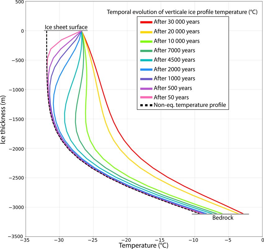
S. Le clec’h et al.: A rapidly converging Greenland ice sheet model initialisation method 2489
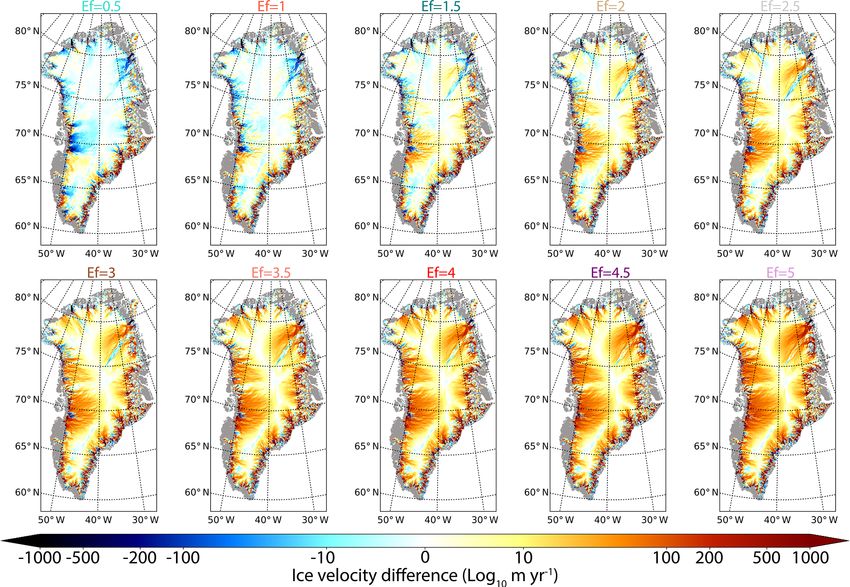
Figure 6. Difference between the simulated and the observed (Bamber et al., 2013) ice thickness (metres) for Ef ranging from 0.5 to 5 for
the iterative cycle Nbcycle that produces the lowest RMSE (Table 1). Here, Nbinv and Nbfree are set to 20 and 200 years respectively.
The ice thickness errors shown in Fig. 6 correspond to a have a poor RMSE (Fig. 5). Also, for Nbcycle = 6, RMSE val-
median value ranging from +15 to −99 m from the lowest ues of Ef = 0.5 and Ef = 2 are close (53.0 m and 52.3 m re-
(Ef = 0.5) to the highest (Ef = 5) enhancement factor. The spectively) but ice volume anomalies are drastically different
decrease in the median of the error with increasing Ef values with 30 738 and −10 254 Gt respectively; see Table 1. Thus,
is mostly driven by the underestimation of the ice thickness a small global ice sheet volume difference does not necessar-
in the interior regions. Our results show that the Ef = 1 ex- ily mean a minimisation of the ice thickness difference.
periment produces the best ice thickness error pattern, rang- For the same reasons, the trend in global ice volume is not
ing from +133 m (5th quantile) to −39 m (95th quantile) and a good metric for assessing the ice sheet drift because lo-
reaching a median error equal to +3 m. cal changes in ice thickness can compensate for each other.
As an illustration, Fig. 9 shows the temporal evolution of
(b) Total ice volume and compensating biases the total ice volume difference for free-evolving simulations
with respect to observations, along with the evolution of the
Because most of the Ef experiments have both positive ice RMSE for a range of enhancement factors. This figure con-
thickness biases at the margins and negative biases over the firms that the GrIS volume equilibrium can be reached by
central part (Fig. 6), the global ice sheet volume is not a good bias compensation as we have a near-zero error in volume
metric for model performance due to compensating biases. with Ef = 1.5 while the RMSE is very similar to that ob-
Figure 8 shows the total ice volume difference with respect tained with Ef = 1 and Ef = 2. For Ef > 2, the negative biases
to observations for varying enhancement factors as a func- in ice thickness dominate, with a decrease in ice volume as
tion of the number of iterative cycles. Some specific exper- Ef increases. For Ef < 2, the positive biases in ice thickness
iments show a very small error in global ice volume with dominate, leading to an increase in the global ice volume.
respect to observations for given Ef values even though they
www.geosci-model-dev.net/12/2481/2019/ Geosci. Model Dev., 12, 2481–2499, 2019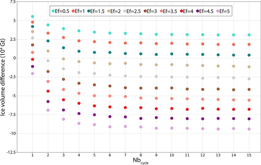
2490 S. Le clec’h et al.: A rapidly converging Greenland ice sheet model initialisation method
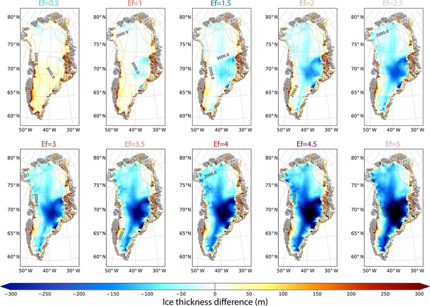
Figure 7. Spatial distribution of the basal drag coefficient (log10 Pa yr m−1 ) for Ef ranging from 0.5 to 5 for the iterative cycle Nbcycle that
produces the lowest RMSE (Table 1). Here, Nbinv and Nbfree are set to 20 and 200 years respectively.
To assess the simulated ice sheet drift and in order to avoid (c) Ice dynamics
the bias compensation, we compute the geometry trend as the
root mean square ice thickness change (ξt – cm yr−1 ): Our iterative minimisation procedure aims to simulate an ice
thickness as close as possible to observations. Hence, the
ξt = [< (Ht − Ht−1 )2 > ]0.5 , (9)
observed ice velocity is not used as a target by the model.
where < (Ht −Ht−1 )2 > represents the averaged squared ice However, because our procedure generates an ice sheet at
thickness change over the whole GrIS. quasi-equilibrium (trend ξ close to 0), the simulated veloci-
Values of ξ computed from the last 5 years of the 200-year ties are close to the balance velocities, which in turn are sup-
free-evolving simulation in the second step (green box in posedly close to present-day observations. As a result, our
Fig. 3) are reported in Table 1 for a given iteration and vary- method simulates an ice flow pattern similar to the observa-
ing enhancement factors. The lowest values are generally ob- tions (Fig. 10).
tained with the experiments that provide the lowest RMSE, The simulated velocity field is particularly sensitive to the
which means that these simulated ice sheets are the closest choice of the enhancement factor (Fig. 10). In particular, for
to equilibrium. The minimal trends are about 15 cm yr−1 and the highest Ef values (Fig. 11), the simulated velocity is over-
are obtained with enhancement factors between 1 and 2. estimated for the major ice streams where deformation due
to vertical shearing is expected to be of less importance com-
pared to basal sliding. For Ef = 1.5, the ice flow pattern in the
margin regions is well reproduced compared to observations
(Fig. 11). Only some glaciers ice velocities can be faster (e.g.
Jakobshavn or Kangerlussuaq) or slower (e.g. Petermann or
Geosci. Model Dev., 12, 2481–2499, 2019 www.geosci-model-dev.net/12/2481/2019/S. Le clec’h et al.: A rapidly converging Greenland ice sheet model initialisation method 2491 Figure 8. GrIS volume difference with regard to observations from Bamber et al. (2013), in gigatons, for Nbinv = 20 years and Nbfree = 200 years and with enhancement factors (Ef) ranging from 0.5 to 5, as a function of the number of iterations (Nbcycle ). Figure 9. Temporal evolution of GrIS total volume difference in gigatons (solid lines) and RMSE (m; dashed lines) for Nbinv = 20 years and Nbfree = 200 years, with varying enhancement factors (Ef) ranging from 0.5 to 5. The Nbcycle chosen here corresponds to the one producing the minimum ice thickness RMSE (see Table 1). www.geosci-model-dev.net/12/2481/2019/ Geosci. Model Dev., 12, 2481–2499, 2019
2492                                 S. Le clec’h et al.: A rapidly converging Greenland ice sheet model initialisation method

                                                                        particular, where the bed is frozen our iterative minimisa-
                                                                        tion procedure is unable to correct for the ice thickness mis-
                                                                        match. This leads to a predominant role of the enhancement
                                                                        factor. The aim of this section is to investigate the sensitiv-
                                                                        ity of our procedure to the initial temperature profile. To this
                                                                        end, we followed the same methodology as in Sect. 4.2, and
                                                                        performed a new set of experiments for which we used an
                                                                        initial temperature profile coming from a previous simulation
                                                                        performed in the framework of the Ice2Sea project (Edwards
                                                                        et al., 2014).
                                                                           This temperature profile differs substantially from the one
                                                                        used in the previous section (black dashed line to be com-
                                                                        pared to the red line in Fig. 12). The temperature profile taken
                                                                        from Edwards et al. (2014) is not consistent with the MAR
                                                                        climatic forcing used for this work and the warmer climatic
                                                                        forcing used here leads to a warmer (about 5 ◦ C) ice sheet
                                                                        compared to the one in Edwards et al. (2014) (Fig. 12). In
Figure 10. (a) Composite ice sheet velocity observation (m yr−1 )
from the NASA Making Earth System Data Records for Use in               the following, the temperature profile taken from Edwards
Research Environments (MEaSUREs) for the 2016–2018 mean pe-             et al. (2014) is referred to as the non-equilibrated tempera-
riod (Joughin et al., 2018). (b) Simulated surface ice velocity using   ture as opposed to the 30 kyr equilibrated temperature used
Ef = 1 for Nbinv = 20 years, Nbfree = 200 years and Nbcycle = 13        in the rest of the paper.
(corresponding to the one producing the minimal ice thickness              Figure 13 shows the evolution of the RMSE for nine it-
RMSE; Table 1).                                                         erative cycles for the experiment performed with the non-
                                                                        equilibrated temperature profile with Ef = 3 (dark blue dots).
                                                                        Similarly to what was shown in Sect. 4.2, the minimisation
Northeast Greenland Ice Stream (i.e. NEGIS)). While the                 procedure reduces the RMSE from +76.0 m after Nbcycle =
best GrIS geometry (lowest RMSE) is obtained with Ef =                  1 to a minimum after Nbcycle = 9 around +47 m. Figure 13
1.5, the experiments with Ef = 1 or Ef = 0.5 best reproduce             also shows the evolution of the RMSE for two experiments
the observed surface velocities (RMSE about 150 m yr−1 ;                with Ef = 1 and Ef = 3 but using the equilibrated temper-
Fig. S1).                                                               ature profile (cyan and orange dots in Fig. 13). While the
   Interestingly the extent of the NEGIS is particularly well           pattern is essentially the same between the different experi-
represented, in particular for lower enhancement factors                ments, the RMSE is higher when using the equilibrated tem-
(Fig. S2). This can be a relic of the long temperature equi-            perature. For the same Ef value, the RMSE is 11.4 m higher
librium performed with a time-constant basal drag coeffi-               (Nbcycle = 8) when using the equilibrated temperature. This
cient taken from Ice2Sea experiments (Edwards et al., 2014),            is because the warmer equilibrated temperature with respect
in which the NEGIS is well delimited (Fig. 2a). However,                to the non-equilibrated one leads to higher velocities which
because this feature is still present when starting the iter-           ultimately favour the ice thickness underestimation in the
ations from a spatially homogeneous basal drag coefficient              central regions (shown in Fig. 6). Using a smaller enhance-
(see Sect. 5.2), it can also suggest that there is some topo-           ment factor with the equilibrated temperature reduces the gap
graphic control of this feature as the adjustment of our local          (3.3 m for Nbcycle = 8) and provides a closer response to that
basal drag coefficient is very effective in reproducing the ob-         obtained for Ef = 3 with the non-equilibrated temperature.
served velocity in this area. Having a good representation of              While the RMSE is lower when the non-equilibrated tem-
the NEGIS is an encouraging sign for the performance of our             perature profile is used, the trend ξ is nonetheless largely
minimisation procedure, especially since most models fail to            higher (24.7 cm yr−1 for Nbcycle = 6) compared to the ex-
achieve this (Goelzer et al., 2018).                                    periments with an equilibrated temperature (16.5 cm yr−1 for
                                                                        Ef = 3 and 16.3 cm yr−1 for Ef = 1 for Nbcycle = 6 and 8 re-
                                                                        spectively). This is expected as there is an important thermal
5     Sensitivity of the method to the initial conditions and           adjustment when using a profile that is not consistent with
      to the duration (Nbinv and Nbfree ) of the                        the climatic forcing.
      minimisation procedure                                               However, despite existing differences to the results ob-
                                                                        tained with the equilibrated temperature profile, this shows
5.1    Sensitivity to the initial temperature profiles                  that our minimisation procedure is able to reduce the mis-
                                                                        match between simulated and observed ice thickness inde-
In Sect. 4.2 we have shown that the results of the minimi-              pendently of the initial temperature profile.
sation are particularly impacted by the basal temperature. In

Geosci. Model Dev., 12, 2481–2499, 2019                                                   www.geosci-model-dev.net/12/2481/2019/
S. Le clec’h et al.: A rapidly converging Greenland ice sheet model initialisation method 2493
Figure 11. Simulated ice surface velocity difference (m yr−1 ) with respect to observations (Joughin et al., 2018) using Ef ranging from 0.5 to
5 for Nbinv = 20 years, Nbfree = 200 years and Nbcycle that corresponds to the one producing the lowest ice thickness RMSE (see Table 1).
5.2 Sensitivity to the initial basal drag coefficient shows that it does not depend on the chosen initial distribu-
tion of the basal drag coefficient.
As explained in Sect. 3, the initial basal drag coefficient β 5.3 Sensitivity to the duration (Nbinv and Nbfree ) of the
for the first iteration of the minimisation procedure is the one minimisation procedure
used in Edwards et al. (2014) (shown in Fig. 2a). To assess
the robustness of our iterative procedure to the choice of the In this section we assess the sensitivity of the minimisa-
initial basal drag coefficient, we have performed a new set of tion procedure to the coefficients Nbinv (i.e. the duration of
experiments starting from a uniform β equal to 1 instead of the period during which the basal drag coefficient is iter-
the one from Edwards et al. (2014). atively computed – first step) and Nbfree (duration of the
Using Nbinv = 20, Nbfree = 200 and Nbcycle varying from free-evolving simulations – second step). While we used
1 to 15 with Ef = 1, we obtain a minimum ice thickness Nbinv = 20 and Nbfree = 200 in Sect. 4.2, here we explore a
RMSE of 49.9 m and a trend ξ of 15.1 cm yr−1 . While there range of combinations of these parameters, testing four val-
are some minor spatial differences in terms of the inferred ues for Nbinv (20, 40, 80, 160 years) and Nbfree (50, 100, 200
basal drag coefficient (Fig. 2c), the aggregated metrics such and 400 years). Using an enhancement factor of 1, we iterate
as the RMSE and the trend are identical to the results pre- 15 cycles (Nbcycle from 1 to 15). The initial conditions are
sented in Table 1. Similarly, the simulated ice thickness and the same as in Sect. 4.2.
surface velocities obtained with β = 1 present very small dif- Figure 14 shows the evolution of the RMSE as a function
ferences compared to those obtained when starting from the of the number of cycles performed for a range of Nbfree val-
Ice2Sea basal drag coefficient (Figs. S3 and S4 in the Sup- ues. As previously shown, there is a strong decrease in RMSE
plement). This illustrates the robustness of the method and between the first two cycles and only a limited improvement
www.geosci-model-dev.net/12/2481/2019/ Geosci. Model Dev., 12, 2481–2499, 20192494 S. Le clec’h et al.: A rapidly converging Greenland ice sheet model initialisation method
Nbcycle = 11. However, this minimum represents a consid-
erable amount of computing time (6160 years) and does
not represent the most efficient combination. As shown in
Figs. 5, 8 and 13, the minimum RMSE generally stabilises
between Nbcycle equal to 4 and 6. This means that simi-
lar RMSE and trend ξ can be obtained using fewer com-
puting resources. For each combination, the mean value of
the best RMSE values is equal to 51.1 m and is associated
with a mean trend ξ of 15.5 cm yr−1 . The experiment with
Nbinv = 20 years, Nbfree = 200 years and Nbcycle = 6 pro-
duces an RMSE 0.6 m lower than the mean and is more than
3 times faster than the best of the RMSE (1320 years com-
pared to 6160 years).
6 Summary and discussion
In order to improve the reliability of Greenland ice sheet sim-
ulations under a future transient climate, an accurate evalua-
tion of the present-day trend of ice flow dynamics is required.
Figure 12. Vertical temperature profiles (◦ C) from the ice sheet One of the major difficulties in addressing this need lies in
surface to the bedrock over the central region of Greenland (73– the poorly constrained observational data of the basal con-
74.5◦ N, 40–43◦ W). The black dashed line is the non-equilibrated ditions that strongly control the ice motion in the entire ice
temperature profile used in Edwards et al. (2014). The coloured sheet. Here, we present an inverse method to infer the spatial
lines are the profiles over the course of the long 30 kyr experiment distribution of the basal drag coefficient in such a way that
for the temperature calculation. The red profile is the one used as
the mismatch between simulated and observed GrIS thick-
the initial condition for the experiments shown in Sect. 4.2.
ness is minimised. As such, our target criteria are defined
for the sets of minimisation procedure parameters providing
minimum values of ice thickness RMSE (with respect to ob-
when using more than six cycles. Using larger Nbfree leads servations) and ice thickness trend, which are respectively as
to a smaller RMSE. This can be explained by the fact that low as ∼ 50 m and 15 cm yr−1 for our best fit. This remains
the correction computed at the end of the second step, after in the range of PDC12 results. The great advantage of the
Nbfree , is greater if the duration of the free-evolving simula- method is its rapid convergence (i.e. 1320 years) making it
tion is longer. This means that the changes imposed on the suitable for more computationally expensive models. More-
new basal drag coefficient computation (Eq. 7) from one cy- over, we have also shown that it only weakly depends on the
cle to another are larger for longer Nbfree . initial guess of the spatial distribution of the basal drag coef-
In Fig. 15 we show the evolution of the RMSE as a func- ficient and the initial temperature profile.
tion of the number of cycles performed for a range of Nbinv Our method, based on the adjustment of the basal sliding,
values (20, 40, 80 and 160 years). The RMSE difference for cannot be applied in regions of frozen bed and is only ef-
a given Nbcycle is generally less than 10 m, while this dif- fective in thawed bed areas where basal sliding may occur.
ference is sometimes larger than 20 m when Nbfree varies However, in case of too large a deformation rate in these re-
from one value to the other. This suggests that Nbinv is of gions, the basal drag coefficient is set to its maximum value
secondary importance relative to Nbfree . The RMSE appears to counteract the overly fast ice flow. The limit of applicabil-
to be slightly smaller for longer Nbinv . For example, for ity of the method led us to investigate the impact of the en-
Nbfree = 200 years, increasing Nbinv from 20 to 40, 80 or hancement factor, which is expected to have a large influence
160 years slightly reduces the minimum RMSE by 0.1, 1.7 or on the deformation rate and, thus, on the ice flow and subse-
3.5 m respectively and decreases the trend ξ by 13.7 %, 7.2 % quently on the simulated ice thickness. We performed a series
and 21.1 % for Nbcycle equal to 12, 11 and 8 respectively. The of simulations with a range of various values of the enhance-
minimum RMSE value (46.1 m) and trend ξ (12.3 cm yr−1 ) ment factor (from 0.5 to 5) and showed that the mismatch be-
are reached with Nbcycle = 10 and with Nbinv = 160 years. tween the simulated and the observed GrIS topography is re-
Performing more cycles once the minimum RMSE is reached duced with an appropriate tuning of the enhancement factor.
does not improve the results. This highlights that the overall performance of the method
Overall, the combination of the highest Nbinv (160 years) is critically dependent on the basal thermal state and high-
with the highest Nbfree (400 years) leads to the small- lights that the finding of appropriate initial conditions with a
est RMSE (44.1 m) with a trend ξ of 9.9 cm yr−1 for simple adjustment procedure remains an undetermined issue.
Geosci. Model Dev., 12, 2481–2499, 2019 www.geosci-model-dev.net/12/2481/2019/S. Le clec’h et al.: A rapidly converging Greenland ice sheet model initialisation method 2495 Figure 13. Ice thickness root mean square error with regard to observations from Bamber et al. (2013), in metres, for Nbinv = 20 years, Nbfree = 200 years, as a function of the number of iterations (Nbinv ). Dark blue dots are for the experiment that uses the non-equilibrated temperature profile as initial condition and Ef = 3. Cyan and orange dots are for the experiments using the equilibrated temperature and Ef = 3 and Ef = 1 respectively. Figure 14. Ice thickness root mean square error with regard to observations from Bamber et al. (2013), in metres, for a fixed Nbinv = 20 and four Nbfree values (50, 100, 200, 400), as a function of the number of iterations (Nbcycle ). The experiments use an enhancement factor of 1. Actually, multiple combinations of the enhancement factor areas. However, we have shown that the minimisation proce- and the basal drag coefficient can produce a simulated ice dure presented in this paper is able to reduce the ice thickness thickness close to the observed one, but this cannot discard mismatch regardless of the initial temperature profile. This the possibility of errors in modelled basal and vertical tem- offers the possibility to tune the thermal state to be as close peratures. A logical next step could lie in the adjustment of as possible to the observations (inferred basal temperature as the basal drag coefficient combined with a similar approach in MacGregor et al. (2016) or vertical profiles at ice core lo- for the adjustment of the enhancement factor in frozen bed cations) before running the iterative minimisation procedure. www.geosci-model-dev.net/12/2481/2019/ Geosci. Model Dev., 12, 2481–2499, 2019
You can also read