A scenario analysis of the 2021-2027 European Cohesion Policy in Bulgaria and its regions - JRC TECHNICAL REPORT

JRC TECHNICAL REPORT

 A scenario analysis of the
 2021-2027 European Cohesion
 Policy in Bulgaria and its regions

 JRC Working Papers on
 Territorial Modelling and Analysis
 No 06/2021

Authors:
Crucitti, F.
Lazarou, N.
Monfort, P.
Salotti, S.

2021 Joint
 Research
 Centre

This publication is a Technical report by the Joint Research Centre (JRC), the European Commission’s science and knowledge service. It
aims to provide evidence-based scientific support to the European policymaking process. The scientific output expressed does not imply a
policy position of the European Commission. Neither the European Commission nor any person acting on behalf of the Commission is
responsible for the use that might be made of this publication. For information on the methodology and quality underlying the data used
in this publication for which the source is neither Eurostat nor other Commission services, users should contact the referenced source. The
designations employed and the presentation of material on the maps do not imply the expression of any opinion whatsoever on the part
of the European Union concerning the legal status of any country, territory, city or area or of its authorities, or concerning the delimitation
of its frontiers or boundaries.

Contact information
Name: Simone Salotti
Address: Edificio Expo, C/Inca Garcilaso 3, 41092 Sevilla (Spain)
Email: simone.salotti@ec.europa.eu
Tel.: +34 954488406

EU Science Hub
https://ec.europa.eu/jrc

JRC126268

Seville: European Commission, 2021

© European Union, 2021

The reuse policy of the European Commission is implemented by the Commission Decision 2011/833/EU of 12 December 2011 on the
reuse of Commission documents (OJ L 330, 14.12.2011, p. 39). Except otherwise noted, the reuse of this document is authorised under
the Creative Commons Attribution 4.0 International (CC BY 4.0) licence (https://creativecommons.org/licenses/by/4.0/). This means that
reuse is allowed provided appropriate credit is given and any changes are indicated. For any use or reproduction of photos or other
material that is not owned by the EU, permission must be sought directly from the copyright holders.

All content © European Union, 2021 (unless otherwise specified)

How to cite this report: Crucitti, F., Lazarou, N., Monfort, P., and Salotti, S. (2021). A scenario analysis of the 2021-2027 European
Cohesion Policy in Bulgaria and its regions. JRC Working Papers on Territorial Modelling and Analysis No. 06/2021, European Commission,
Seville, JRC126268.
The JRC Working Papers on Territorial Modelling and Analysis are published under the supervision of Simone Salotti and Andrea
Conte of JRC Seville, European Commission. This series mainly addresses the economic analysis related to the regional and territorial
policies carried out in the European Union. The Working Papers of the series are mainly targeted to policy analysts and to the academic
community and are to be considered as early-stage scientific papers containing relevant policy implications. They are meant to
communicate to a broad audience preliminary research findings and to generate a debate and attract feedback for further improvements.

A scenario analysis of the 2021-2027 European Cohesion Policy in Bulgaria and its regions

 Francesca Crucittia, Nicholas-Joseph Lazaroua, Philippe Monfortb, and Simone Salottia
 a
 European Commission, Joint Research Centre (JRC), Seville, Spain
 b
 European Commission, DG for Regional and Urban Policy (DG REGIO), Brussels, Belgium

Abstract

We employ the spatial dynamic general equilibrium model RHOMOLO to estimate the economic
impact of the 2021-2027 Cohesion Policy in Bulgarian NUTS-2 regions and analyse the implications
for growth and development in Bulgaria. The main investment areas covered by the policy fall into
the following five fields of intervention: aid to the private sector, research and development,
transport infrastructure, other infrastructure, and human capital. They are characterised by a
varying degree of positive demand and supply side effects on regional and aggregate development,
which, together with the level of the shocks, determine the impact on GDP. We find that a projected
€10.9 billion of Cohesion Policy funding would increase Bulgarian GDP by 3.4% above its baseline
value at the end of the implementation period in 2030 and by 2.4% ten years later. Our results
suggest that there is no systematic equity-efficiency trade-off in Bulgaria which mainly arises as the
consequence of low spillovers in the capital city region versus the strictly higher spillovers observed
in the rest of the country’s regions. We conclude that a balanced Cohesion Policy portfolio would
foster a high impact on national GDP, maintain a high intensity of spillovers and reduce regional
disparities in Bulgaria.

JEL Codes: C68, R13.

Keywords: RHOMOLO, Cohesion Policy, regional growth, regional development, Bulgaria.

1. Introduction

We estimate the potential economic impact of a hypothetical European Union (EU) Cohesion Policy
funding for the period 2021-2027 in Bulgaria and study its implications for growth and development
for the country and its NUTS 2 regions. For this purpose we employ RHOMOLO, a dynamic spatial
computable general equilibrium (CGE) model for EU regions and sectors, developed by the European
Commission for territorial impact assessment.

The EU Cohesion Policy is the EU's main investment policy. It aims to strengthen economic and social
cohesion by reducing disparities in the level of development between regions by supporting job
creation, business competitiveness, economic growth, sustainable development, and improving
citizens’ quality of life.1 The funding is delivered to regions through two main funds, the European
Regional Development Fund (ERDF, 43% of Cohesion Policy) and the Cohesion Fund (CF, 13%).
Together with the European Social Fund (ESF, 18%), the European Agricultural Fund for Rural
Development (EAFRD, 22%) and the European Maritime and Fisheries Fund (EMFF, 1%), they
comprise the European Structural and Investment Funds (ESIF). In order to facilitate the
implementation of the Green Deal, the Just Transition Fund (JTF) was recently launched as the new
financial instrument within the 2021-2027 Cohesion Policy with a budget of €17.5 billion, aiming to
provide support to territories facing serious socio-economic challenges arising from the transition
towards climate neutrality. Around 70% of the resources go to the economic, social and territorial
cohesion objective, with more than half of that targeting less developed regions where GDP is less
than 75% of the EU average.

The aim of this paper is to analyse the potential impact of the 2021-2027 ERDF, CF, ESF (including
the Youth Employment Initiative), and JTF in Bulgaria, a Member State which for the 2014-2020
programming period was allocated 7.72 billion of EU resources under those three Funds (and more
than 10 billion including the other two funds of ESIF). This Cohesion Policy funding was used for the
implementation of investments that increased environmental protection, upgraded infrastructure,
promoted educational and vocational training, research and development and social inclusion inter
alia.

Based on consultations with the Bulgarian authorities on the draft Partnership Agreement, we
obtain the most up to date information regarding the amount allocated to Bulgaria for the 2021-
2027 programming period and the breakdown of the funding into various investment priorities. In
order to get a full picture for the impact assessment analysis, this information was integrated with
data for the previous programming period on the geographical distribution of funding across the
country’s NUTS 2 regions, and on the expected time profile of expenditure which is spread over ten
years, from 2021 to 2030).2 This permits us to construct a baseline scenario generating a potential
macroeconomic impact in the country with a certain variation across its regions. Investments
supported by the EU funding are likely to generate spatial spillovers, as programmes implemented in
a given region could affect the other regions of the country as well. The economic impact of the

1
 In order to reach these goals and address the diverse development needs in all EU regions, € 355.1 billion –
almost a third of the total EU budget – has been set aside for Cohesion Policy for the programming period
2014-2020. (https://ec.europa.eu/regional_policy/index.cfm/en/policy/what/investment-policy/). The exact
budget for the 2021-2027 period is being negotiated at the time of writing (July 2021).
2
 The implementation period exceeds the seven year programming period by three years as cohesion policy
allocations, which are divided into annual tranches, must be spent within two or three years. This is referred as
the N+2 or N+3 rule, with N being the start year when the money is allocated.

policy therefore ultimately depends on how the funding is distributed among the country’s regions
and among the fields of intervention. This is analysed by addressing four additional policy questions
which showcase the variation in the regional and aggregate policy impact and could assist the policy
maker in designing the investment portfolio when targeting mitigation of regional disparities or
boosting economic activity across regions.

We use the dynamic spatial general equilibrium model RHOMOLO to estimate the macroeconomic
effects of the Cohesion Policy interventions in Bulgarian regions. The structure of the model –
calibrated based on data for 267 NUTS 2 regions of the EU27 + the UK – makes it a suitable tool for
evaluating policies implemented at the regional level, as well as for evaluating the territorial impact
of policies implemented at the national and European levels. Economic models like RHOMOLO are
routinely used for policy impact assessments and evaluations (see for example Barbero et al., 2021;
Barbero and Salotti, 2021; Conte et al., 2020; and Lecca et al., 2020). Ex-ante evaluations are carried
out prior to policy implementation, and inform the decision-taking process with regards to the
selection of alternative policy designs.

We find that a projected €10.9 billion of Cohesion Policy funding for 2021-2027 has the capacity to
increase Bulgarian GDP by 3.4% above its baseline value in 2030 (at the end of the implementation
period) and by 2.4% ten years later. We identify that a balanced distribution of investments in aid to
the private sector, infrastructure and research and development may lead to the mitigation of
regional disparities in Bulgaria. The capital city region is the most developed region of Bulgaria and,
according to our simulations, it provides high investment returns in almost all fields of intervention.
However, given the relatively low level of generated spillovers of investments there, concentrating
resources in that region may lead to amplification of regional disparities and would not necessarily
lead to the best economic performance for the whole country. In fact, the results suggest that there
is no systematic equity-efficiency trade-off in Bulgaria, which mainly arises as the consequence of
low spillovers in the capital city region versus the strictly higher spillovers in the rest of the country’s
regions. It is therefore possible to design a policy portfolio which produces a high impact on national
GDP while at the same time contributing to reduce regional disparities within the country.

The remainder of this paper is structured as follows: Section 2 describes the Bulgarian economy and
the distribution of 2021-2027 Cohesion Policy funding across Bulgarian NUTS 2 regions and
investment priorities. Section 3 provides an overview of RHOMOLO and the modelling of
investments depending on the policy questions so as to run the model. Section 4 analyses the
baseline scenario and addresses the policy questions. Section 5 concludes.

2. The Bulgarian Economy and the 2021-2027 Cohesion funding distribution

2.1 Country Background

Table 1 lists the country and regional statistics at the NUTS 2 level of regional disaggregation for year
2018.3 The capital city region, BG41, is by far the most developed of the country, with GDP per head
corresponding to around 82.3% of the EU average. The GDP per head of the other regions ranges
between 33.1% and 41.6% of the EU average. Recently, GDP growth has been slower in the less
developed regions (with the exception of BG34 and BG42), which implies that internal regional
disparities are growing over time.

3
 The latest year that does not include projections.

Table 1. Economic Indicators of Bulgarian NUTS 2 regions
 Real GDP % Change in 2021-
 growth, real income 2027
 2008- Employm of Cohesion
 GDP per 2018, Populatio ent Income of Households 2014-2020 Funding
 capita annual n (2018, (2018, Households (2008-2018, Cohesion (provisio
 2018, EU- average thousand thousand (2018, mln %) Funding nal, mln
 Region 28=100 (%) s) s) €) (mln €) €)

 10,894.9
Bulgaria (BG) 51.0 1.9% 7,050 3,068.9 33,609.08 +78% 7,630.82 6
Severozapaden
(BG31) 33.1 0.8% 755.9 266.3 2,217.34 +34% 879.35 1,279.29
Severen
tsentralen
(BG32) 34.5 1.0% 794.9 323.7 2,829.84 +47% 899.49 1,295.68
Severoiztoche 999.36
n (BG33) 40.7 1.3% 933.7 397 3,449.37 +67% 1,422.53
Yugoiztochen
(BG34) 41.6 2.5% 1,039.5 438.5 3,944.7 +54% 1,104.13 1,572.93
Yugozapaden
(BG41)* 82.3 2.1% 2,108.3 1,034.3 15,977.43 +119% 2,217.56 3,136.76
Yuzhen
tsentralen
(BG42) 35.8 2.1% 1,417.4 609.2 5,190.39 +56% 1,530.94 2,187.77
Source: Eurostat and DG REGIO (Cohesion Funding data). *Capital city region.

A number of features of the regional economies will likely drive the nature of the impact of Cohesion
Policy interventions. In particular, the following three stand out: the level of development, trade
openness (and in particular the propensity to import), and the intensity in the usage of production
factors.

In Table 2, trade openness is proxied by the share of imports over output for each NUTS 2 region of
Bulgaria. The table also reports the percentage of imports coming from each of the other regions in
Bulgaria with respect to the total imports of the region.
Table 2. Share of imports in output and regional share of imports from the rest of the Bulgarian regions.
 BG31 BG32 BG33 BG34 BG41 BG42
Imports/output 24% 27% 44% 54% 86% 63%
BG31 4% 4% 2% 2% 2%
BG32 13% 18% 2% 1% 2%
BG33 5% 8% 3% 2% 2%
BG34 13% 7% 5% 2% 5%
BG41 22% 23% 13% 9% 11%
BG42 12% 7% 4% 5% 3%
TOTAL 65% 50% 44% 22% 9% 23%
Source: RHOMOLO.

The capital city region BG41 is by far the most open to international trade, as it mostly trades with
partners outside Bulgaria and only 9% of its imports come from the rest of the country. This
contrasts with the less developed regions whose trade is to a much larger extent intra-country in
nature, the capital city region being the relatively most important source of imports. For instance,
65% of BG31 imports come from other regions of the country, and 22% from the capital city region.

The technology in the Bulgarian regions differs widely from one another and reflects their industrial
fabric. In particular, the capital city region is much more labour intensive than the other regions in
which the predominant sector of activity is not constituted by services as much as in BG41.
Table 3. Share of labour (vs capital) in GDP
Region BG31 BG32 BG33 BG34 BG41 BG42
Labour share 55.2% 48.2% 49.8% 52.5% 71.1% 58.2%
Source: RHOMOLO.

2.2 The 2021-2027 Cohesion Policy in Bulgaria

Based on the October 2020 draft of the Partnership Agreement, the Cohesion Policy investments
allocated to Bulgaria for the 2021-2027 programming period stand at €10.9 billion. The draft
Agreement contains the breakdown of the funding between five Priority Objectives (PO1: Smarter
Europe; PO2: Greener, low carbon Europe; PO3: More connected Europe; PO4: More social Europe;
and PO5: Europe closer to citizens), technical assistance, and the JTF as per Figure 1. For the 2021-
2027 programming period, each Priority Objective is broken down into a series of Specific Objectives
(SOs) which reflects the nature of the interventions envisaged. Currently, and in the absence of
information regarding the distribution of the funding among the SOs, we assume that the amount
under each Priority Objective is equally shared among the SOs covered by each Priority Objective.
Therefore there are 23 SOs corresponding to 5 Priority Objectives, 12 ESF areas of intervention (all
listed under SO 4.1), technical assistance and the Just Transition Fund (the full list of SOs can be
found in the Appendix).
Figure 1. Breakdown of Cohesion funding across Priority Objectives.

 3%
 11% 16%

 14%
 22%

 23%
 12%

 PO1 PO2 PO3 PO4 (European Social Fund) PO5 Technical Assistance Just Transition Fund

Source: DG REGIO. Please note that this breakdown is based on an early draft of the Partnership Agreement
and will most certainly change before the Agreement is finalised.

At this stage two assumptions need to be introduced as ingredients to the model. First, the
geographical breakdown of the funding among the NUTS 2 regions of Bulgaria is assumed to be the
same as for the 2014-2020 period (see Table 4). Second, it is assumed that regional funding under
each SO is distributed accordingly. Likewise, the time profile of expenditure of the funds is taken
from the one established for the 2014-2020 programming period at the country level as per Table 5.
We refer to this allocation as the baseline scenario in the rest of the Report. The simulation strategy
adopted to quantify the effects of the investments is described in the following Section, together
with a brief presentation of the RHOMOLO model.
Table 4. Geographical breakdown of expenditure
 Region BG31 BG32 BG33 BG34 BG41 BG42 Total
 Share 11.7% 11.9% 13.1% 14.4% 28.8% 20.1% 100.0%
Source: DG REGIO.

Table 5. Time profile of expenditure
Year 2021 2022 2023 2024 2025 2026 2027 2028 2029 2030
Share of total expenditure 2.3% 4.7% 7.9% 11.2% 14.2% 16.7% 17.7% 14.7% 8.8% 1.7%
Source: DG REGIO.

3. The RHOMOLO model and modelling Cohesion Policy in Bulgaria

3.1 A brief overview of the model

RHOMOLO is a dynamic spatial computable general equilibrium model whose purpose is to provide
analyses with sector-, region-, and time-specific results related to investment policies and structural
reforms in the EU. The model is calibrated on a set of fully integrated EU regional Social Accounting
Matrices (SAMs) for the year 2013 which is taken as the baseline state of the economy. The SAMs
account for all the transactions in the economy: purchasing of intermediate goods, hiring of factors,
and current account transactions of institutions including taxes and transfers, consumption and
savings, as well as trade flows. A SAM includes more information than a simple Input-Output (IO)
table (which contains information on the production and use of goods and services and the income
generated in that production), as it includes data on the secondary distribution of income, detailing
the roles of labour and households (Miller and Blair, 2009).

The main distinctive feature of the model lies in its regional dimension, as it is calibrated with data
for 267 NUTS 2 regions of the EU27 + the UK, as well as for a residual region accounting for the rest
of the World (Thissen et al., 2019). Thus, the model is well-equipped to analyse the territorial impact
of funding programmes and policies, especially those with a marked geographical focus such as the
EU Cohesion Policy.

The full mathematical description of the RHOMOLO model is beyond the scope of the present
Report and can be found in Lecca et al. (2018). Succinctly, the model economies are disaggregated
into ten economic sectors (based on the NACE Rev. 2 industry classification), and firms are assumed
to maximise profits and produce goods and services according to a constant elasticity of substitution
production function. The remaining agents in the model include utility-maximising households and a
government which collects taxes and spends money on public goods and transfers. Capital and
labour are used as factors of production, and transport costs are based on the transport cost model
by Persyn et al. (2020). The model is solved in a recursively dynamic mode, where a sequence of
static equilibria is linked to each other through the law of motion of state variables. This implies that
economic agents are not forward-looking and their decisions are solely based on current and past
information.

The next sub-section is devoted to the illustration of how the Cohesion Policy investments are
introduced into the model in order to simulate their effects on the economy. Essentially, the
detailed information on the SOs of the 2021-2027 Cohesion funding must be simplified and
translated into modelling shocks. This allows us to construct scenarios in which the state of the
economy changes according to specific economic mechanisms which are specific to the type of
intervention simulated, such as aid to private sector or investments in transport infrastructures.

3.2 Translating Cohesion Policy expenditures into model shocks

For the purposes of the analysis, we grouped the 37 spending categories (corresponding to the 35
SOs, technical assistance and the Just Transition Fund) into the following six fields of interventions:
Transport infrastructure investments (TRNSP); other infrastructures (INFR); investments in human

capital (HC); investments in research and innovation (RTD); aid to the private sector (AIS); and
 technical assistance (TA).4

 Each spending category was assigned to a model shock to simulate an appropriate, identified
 economic impact, resulting in the fields of interventions being modelled either with single shocks, or
 with combinations of shocks according to the nature of the interventions. The breakdown by field of
 intervention and model shock is presented in Table 6 along with a brief description of the nature of
 the shock that is assumed in the RHOMOLO model. The demand-side effects are temporary in nature
 and reflect the transfer of resources resulting from the implementation of the Cohesion Policy
 package. The supply-side effects are structural and capture the long-lasting changes stemming from
 each policy intervention. The associated labels of the SOs can be found in Appendix A. We now
 describe the specificities of each of the fields of intervention represented by model shocks.
 Table 6. Definition of Fields of Intervention and model shocks
 Field of Share of
Field of Model Demand-side
 intervention Supply-side effects 2021-2027
intervention shock effects
 Label expenditure
Transport Increase in public Decrease in transportation 11.6%
 TRNSP TRNSP
infrastructures consumption costs
 Increase in public Temporary increase in the
 IG (50%)
 investment stock of public capital (5%
Other
 INFR depreciation rate) 49.5%
infrastructures
 Increase in public
 G (50%)
 consumption
 Increase in labour
 Increase in public
Human Capital HC HC productivity
 consumption 23.1%
 (75% of the HC expenditure)

Research and Stimulates private Increase in total factor
 RTD RTD 6.2%
Development investment productivity (TFP)
 Temporary increase in the
 Reduction in risk stock of private capital (15%
 premium depreciation rate) (100% of
Aid to private
 AIS RPREMK stimulating the AIS expenditure) 6.2%
sector
 private
 investment Increase in TFP (only 50% of
 the AIS expenditure)
Technical Increase in public 3.3%
 TA G
assistance consumption
 Source: RHOMOLO modelling assumptions and DG REGIO.

 Transport infrastructures (TRNSP) - The resources allocated to transport infrastructure are assumed
 to generate temporary effects through increases in government consumption in order to account for
 the purchase of goods and services required to build the actual infrastructures. The associated
 supply-side and long-lasting effect is simulated through a reduction in transport cost stimulating
 trade flows. Transport costs affect all ten economic sectors considered in the model. The estimated

 4
 Technical Assistance to Bulgaria is not considered in the analysis as the demand for it, as well as the nature
 and content of any intervention is unknown. Additionally the amount reserved for it (3.3% of the Cohesion
 Policy budget) is very small.

reduction in costs due to Cohesion Policy investments is calculated with a linear approximation of
the impact of comparable transport investments estimated with the transport cost model by Persyn
et al. (2020).

Other infrastructures (INFR) - Regional investments in non-transport infrastructures are typically
related to electricity networks improvements, water treatment, and waste management. These are
modelled and implemented in RHOMOLO either as a public investments (IG - when associated with
industrial processes) or as a government consumption (G). The IG shock is implemented as an
exogenous increase in public investment augmenting the amount of the public capital stock, which
enters the production function of the model as an unpaid factor.

Investment in human capital (HC) - The implementation of human capital policies is modelled in
RHOMOLO as follows. First of all, in the short run all the HC expenditures are modelled as
government current expenditure. Then, in order to model the long-run productivity-enhancing
effects of the policy, we calculate the additional school year-equivalents of training that can be
purchased with the Cohesion Policy investment in human capital in each region and for each labour
skill-group (low, medium, and high). This allows to compute the change in school years embedded in
the labour force due to the policy. Then, following the empirical literature on Mincer-type
regressions (Card, 2001), labour efficiency is assumed to increase by 7% for each additional school
year gained, with country-specific adjustments related to the PISA score accounting for different
returns to education.

A key piece of the required information is the cost per pupil of different levels of schooling, which is
obtained from Eurostat. These data are used as an estimate of how much one year of additional
training would cost to train one worker in each of the three skill groups. We take one year of the
tertiary-level education as the cost of training for all skill levels, because the majority of the
Cohesion Policy investment in the human capital aims at training workers.

Research and development (RTD) - This expenditure is implemented in RHOMOLO trough a
temporary increase in private investment stimulated by a reduction in risk premium (which in turn
affects the user cost of capital) to reflect the firms’ investments in R&D activities. The supply-side
permanent effects associated to this policy are simulated through a TFP improvement. The money
injection is translated into TFP shocks via an elasticity estimated with a model à la Kancs and
Siliverstovs (2016). The elasticity depends positively on the R&D intensity of each region, a data
retrieved from Eurostat.

Aid to private sector (AIS) - Cohesion Policy supports investors who want to engage in risky activities
with a high potential for fostering economic growth and employment. These investments are
assumed to stimulate private investments via a reduction in the risk premium and, therefore, in the
user cost of capital (RPREMK). 50% of the AIS spending is assumed to have productivity-enhancing
effects as in the case of RTD.

Technical assistance (TA) - This investment on the economy is modelled as an increase in public
current expenditure (G) to account for purchases of goods and services associated with the transfer
of resources, with no associated supply-side effects. This field of intervention is not discussed in this
paper.

It should be noted that all the supply-side long-run effects decay over time. The stocks of public and
private capital depreciate at a 5% and 15% yearly rate, respectively, and both the productivity
improvements and the transport cost reductions also decay at a 5% yearly rate. The reason behind
this assumption is that even research and development breakthroughs leading to productivity

improvements eventually cease to represent an advantage for the regional economy which benefit
from them. Also, the model takes into account the fact that the Cohesion Policy is financed by the
EU budget to which each Member State contributes proportionally to its GDP, the national
contribution being financed through lump-sum taxes in RHOMOLO. The latter decrease household
disposable income, thus adversely affecting the economic performance and partly offsetting the
positive impact of the programmes.
4. Simulation Strategy and Results

Our simulations are based on a set of policy relevant questions developed in collaboration with DG
REGIO (Table 7). Besides the first question on the effects of the specific interventions, the rest of the
questions aim to identify the impact of redistributing funding across the regions, or SOs, or
combinations of both, starting from the baseline scenario in which funds are distributed across SOs
and regions as described in sub-section 2.2. The second column of the table reports the sections of
the paper dealing with each question.
Table 7. Policy questions on the impact of 2021-2027 Cohesion Policy in Bulgaria

Q1 S. 4.2 Which field of intervention would trigger the highest GDP impact in which region(s)?

Q2 S. 4.3 What would be the impact of distributing half of the transport budget to the different regions
 equally compared to the baseline situation?

Q3 S. 4.4 What would be the impact of distributing half of the energy efficiency budget to the different
 regions equally compared to the baseline situation?

Q4 S. 4.5 What would be the impact of significantly increasing the transport or energy efficiency
 allocation for the two least developed regions?

By employing the RHOMOLO model we can establish how the reallocations envisaged in questions 2
to 4 affect the impact of the policy on the country’s and the regional economies. This can yield
valuable information for the European and Bulgarian policy makers in the context of designing the
2021-2027 Cohesion Policy programmes. The questions are answered relative to the baseline
scenario which reflects the simultaneous expenditure of funds across fields of intervention and
Bulgarian regions. Before tackling the four policy questions of Table 7, we assess (in sub-section 4.1)
the potential impact of the hypothetical investments portfolio illustrated above relative to the no
policy scenario. We then present the results corresponding to each question and discuss their policy
implications.
4.1. The baseline scenario
RHOMOLO is a general equilibrium model and therefore each simulation produces a large amount of
results. Thus, choices must be made in order to present the most relevant information specific to the
research question addressed by each analysis. In this case, we concentrate firstly on the GDP impact
and then on the GDP multipliers. The GDP impact is expressed as the percentage difference relative
to no policy scenario. 2030 is the last year in which Cohesion Policy investments are made and can
be considered as the short run in which the GDP impact mainly reflects the demand side effects
described in Table 6. The supply-side effects are also at work, but their effects die out much later.
The results for 2040 can be interpreted as the long run impacts of the policy since starting from 2030
only the supply side or structural aspects remain. These effects pertain to changes in productivity
and transportation costs. Some residual demand side effects remain: for example, the public capital
stock depreciates slowly so that the effects of public investments can still be felt in the regional
economies ten years after the end of the implementation period. Figure 2 shows the impact on GDP

in 2030 and in 20405, as well as the magnitude of the Cohesion Policy investments with respect to
GDP, in the Bulgarian regions and in the country as a whole.
Figure 2. Impact on GDP in 2030 (I10) and 2040 (I20) as % differences from no-policy-scenario GDP (lhs scale), and Cohesion
Policy expenditure as % of GDP (yearly average - rhs scale)
 5.00 0.60%

 4.50
 0.50%
 4.00

 3.50
 0.40%
 3.00
 I10
 2.50 0.30%
 I20
 2.00
 Exp as % of GDP
 0.20%
 1.50

 1.00
 0.10%
 0.50

 0.00 0.00%
 BG31 BG32 BG33 BG34 BG41 BG42 BG

Source: RHOMOLO simulations.

The magnitude of the impact closely follows that of the policy injection in the regional economy. In
the short-run, the highest impact is in BG31 where GDP in 2030 is around 4.6% higher than in the
absence of the programmes. During the implementation period, Cohesion Policy expenditure in
BG31 corresponds on average to 0.5% of regional GDP per year. In BG41, the impact is only 2.8%
above the no-policy-scenario at the end of the implementation period, but expenditure corresponds
to 0.2% of yearly GDP on average. This is not surprising, as in the short run the impact on GDP is
mostly driven by the demand side shocks of increased investment and current expenditure. In the
longer run, the importance of supply-side effects increases with respect to that of the demand-side
ones, thus the picture changes slightly (for instance, the impacts in BG31 and BG32 differ more in
2040 than in 2030).

Table 8 reports the impact on GDP in 2030 and 2040 in columns I10 and I20 respectively, and the
GDP multipliers in 2030 and 2040 in columns M10 and M20. The latter are defined as the cumulated
changes in GDP in absolute values divided by the full amount of the policy investments. For instance,
a multiplier of 1.5 means that for each euro spent through the policy, GDP increases by 1.5 euro. The
last column reports the average amount of Cohesion Policy allocation with respect to yearly GDP
during the implementation period.
Table 8. Impact on GDP in 2030 (I10) and 2040 (I20) expressed as % differences from no-policy-scenario GDP, multipliers in
2030 (M10) and 2040 (M20), and Cohesion Policy expenditure as % of GDP (yearly average)
 BAU I10 I20 M10 M20 Expenditure as % GDP
 BG31 4.64 3.20 0.80 1.58 0.5%
 BG32 4.63 3.55 0.83 1.83 0.4%
 BG33 3.74 2.95 0.88 1.97 0.3%
 BG34 3.53 2.67 0.84 1.82 0.3%
 BG41 2.85 1.85 1.27 2.59 0.2%

5
 I10 and I20, respectively: 10 and 20 stand for the years after the beginning of the policy implementation.

BG42 3.80 2.66 0.78 1.59 0.4%
 BG 3.44 2.43 0.95 1.99 0.3%
Source: RHOMOLO simulations.

The multiplier is the highest in BG41 where 1 euro invested through Cohesion Policy returns 2.6
euros in GDP after 20 years. This is to a large extent due to some of the characteristics of the capital
city region which are analysed in detail in the next Section but it is also due to the fact that the
region is the one benefitting most from positive spillovers originating in other regions of the country.
While in 2030 the multiplier is lower than one in most of Bulgaria, it is largely above one by 2040.
This reflects the fact that, due to its substantial supply-side effects, the benefits of Cohesion Policy
continue after the end of the programmes, highlighting the structural effects of the policy in the
medium to long run.

4.2. Q1: Which spending category would produce the highest GDP impact in which region(s)?
We perform two sets of experiments to answer to this question. First, we run individual simulations
per field of intervention simultaneously across all regions to identify the region in which the highest
GDP impact is produced. Second, we simulate region-specific investments to identify which region of
the country generates the highest GDP impact for Bulgaria as a whole when targeted by Cohesion
Policy investments.

For the first case, the shocks occur simultaneously in all Bulgarian regions and the regional GDP
multipliers are reported in Table 9. For each field of intervention, the multipliers are calculated both
at the end of the implementation period of the policy (10 years), and ten years afterwards (20
years). For the shocks with substantial supply-side effects, like infrastructure investments, it is more
meaningful to look at the long run impact on GDP rather than at the effects in the short run only.
Table 9. Regional GDP multipliers - country-wide shocks
 AIS RTD INFR TRNSP HC
 10 yrs 20 yrs 10 yrs 20 yrs 10 yrs 20 yrs 10 yrs 20 yrs 10 yrs 20 yrs
BG31 0.80 1.85 0.86 2.01 0.94 1.90 0.57 0.63 0.70 1.37
BG32 0.84 2.03 0.91 2.25 0.98 2.30 0.66 0.81 0.61 1.37
BG33 0.86 2.16 0.95 2.44 1.05 2.44 0.66 0.84 0.67 1.53
BG34 0.88 2.12 0.97 2.38 0.99 2.20 0.56 0.66 0.70 1.57
BG41 1.04 2.38 1.18 2.76 1.37 2.85 1.34 1.71 1.20 2.72
BG42 0.85 1.97 0.94 2.22 0.88 1.87 0.65 0.78 0.63 1.33
Source: RHOMOLO

Important regional differences in the multipliers for all fields of intervention arise, with AIS being the
field characterised by the narrowest range of multipliers.6 The capital region BG41 tends to have the
biggest economic impact from the funding shocks, however in the cases of AIS and RTD the
differences with the rest of the regions are not large. The TRNSP and HC fields exhibit the largest
variation between BG41 and the other regions. One explanation for the large impact of transport
infrastructure investments in BG41 lies in its trade openness (see Table 2 above): reducing transport

6
 Differences in the values of the multipliers may seem small but they actually correspond to significant
differences in terms of returns. For instance, the 20 year RTD multiplier of BG31, 2.01, yields an compound
annual rate of return of 3.5%, whilst the RTD multiplier for BG41, 2.76, corresponds to a rate of 5.2% per
annum respectively, according to: , = 1/( − 0) − 1, where t is the year after the policy
implementation in region r and t0 refers to the year before the policy implementation.

costs in that region significantly benefits GDP because it affects a large volume of trade flows. Given
the intense economic activity of the region, it is also possible that the benefits are generated via
reduced costs of within-region flows of goods and services.

Returns on investments in human capital are particularly high in BG41. This is due to the fact that
technology in the capital city region is more intensive in labour, and in particular skilled labour, than
in the other regions and increasing the stock of this production factor has therefore a bigger impact
on GDP.7 The data also suggest a positive correlation between the HC (and RTD) multipliers and the
level of development (measured by GDP per capita) as highlighted by Figure 3.

Figure 3. RTD and HC 20 years multipliers vs GDP per head

 2.80
 Multiplier at year 20

 2.50

 2.20

 1.90

 1.60

 1.30

 1.00
 30 40 50 60 70 80 90
 GDP per head (PPs), EU 28 = 100
 RTD HC

Source: EUROSTAT and RHOMOLO.

The reasons for this positive correlation are mostly linked to the specificities of the industrial fabric
of the various regions. The capital city region hosts more R&D intensity activities than the other
regions of Bulgaria, at least twice as much as in the other regions.8 In 2018, 7.9% of the employment
was in the high-technology sectors and 39.6% in knowledge intensive services, also higher than in
the rest of the country. As highlighted in the literature (see for instance Kancs and Siliverstovs,
2016), the impact of R&D investments on firm productivity is likely to be higher in places with high
levels of R&D intensity and the impact of R&D investments is therefore higher in this region.
Regarding investments in human capital, labour intensive technology in the capital city region
(especially medium to high skill labour) explains why the return on investments in human capital is
between two or three times the magnitude observed in other regions. Yet this should not prevent
investment in R&D and human capital from being ingredients of a good development policy in all
Bulgarian regions, including the less developed ones. R&D investments in more developed regions
may promote frontier research activities, but R&D also covers activities such as production processes
and market and/or organisational innovation relevant for economic agents in less developed regions
as well. This explains why the impact of R&D investment is the largest in BG41, but it is significant in
other regions as well.

7
 This effect is the equivalent to the Rybczynski (1955) theorem within RHOMOLO.
8
 In 2018, R&D intensity activities over GDP in BG41 was 1.1% versus the other regions ranging between 0.3%
and 0.5% (source: Eurostat).

Table 10 contains both the regional and country GDP 20 years multipliers corresponding to the
second set of experiments, where a particular funding shock is simulated in one region at a time (the
country multipliers are calculated by dividing the sum of the changes in GDP in all the regions of the
country, including the ones that are not shocked, by the region-specific investment). This allows to
quantify the effects in the region, and also to identify any spillover effects to the rest of the
Bulgarian regions stemming from the region-specific investments.9
Table 10. Regional and country GDP multipliers (20 years) - region-specific shocks
 AIS RTD INFR TRNSP HC
 Reg Cnt Reg Cnt Reg Cnt Reg Cnt Reg Cnt
BG31 1.70 2.06 1.86 2.22 1.70 2.18 0.45 0.91 1.24 1.62
BG32 1.81 2.19 2.02 2.42 2.05 2.59 0.60 1.03 1.20 1.58
BG33 1.88 2.22 2.15 2.50 2.11 2.56 0.56 0.89 1.28 1.58
BG34 1.86 2.20 2.11 2.47 1.89 2.32 0.44 0.77 1.33 1.65
BG41 1.96 2.06 2.32 2.43 2.25 2.39 1.22 1.34 2.26 2.37
BG42 1.80 2.11 2.04 2.36 1.65 2.03 0.59 0.91 1.16 1.46
Source: RHOMOLO

The regional multipliers of Table 10 suggest that RTD investments would trigger the highest impact
in all Bulgarian regions compared to the other fields of intervention, with slightly larger effects in the
capital city region BG41. These results confirm that HC investments would lead to a much higher
GDP response in BG41 compared to the rest of the country. Turning to the country multipliers,
investing in the capital region BG41 does not necessarily result in the highest country-level GDP
multiplier, except for the case of HC and TRNSP. In all the other cases, the impact of the policy on
the country’s GDP is maximised when a region other than BG41 is shocked, namely BG33 in the case
of AIS and RTD, and BG32 for INFR. This result stems from the substantial spillover effects which are
usually larger when less developed regions are shocked. This is highlighted in Table 11 which
contains the spillovers expressed as percentage of the country multipliers of Table 10.
Table 11. Spillovers expressed as % of country GDP multipliers (20 years) - region-specific shocks
 AIS RTD INFR TRNSP HC
BG31 17% 16% 22% 51% 23%
BG32 17% 17% 21% 42% 24%
BG33 15% 14% 18% 37% 19%
BG34 15% 15% 19% 43% 19%
BG41 5% 5% 6% 10% 5%
BG42 15% 14% 19% 35% 21%
Source: RHOMOLO

Table 11 shows that investments in the less developed regions generally generate larger spillover
effects. For example, between 14% and 17% of the AIS and RTD country multipliers are due to
spillovers when regions other than BG41 are shocked. That number is only 5% when the RTD
investments target BG41. The equivalent share for INFR is 18-22% relative to only 6% for BG41. In
fact, investments in the capital region generate the smallest spillovers to the rest of the country,
irrespective of the type of shock considered. The reason is that less developed regions have a higher
propensity to import goods and services from other Bulgarian regions because they have less
capacity to satisfy the Cohesion Policy-related demand with their own production. Typically, the
capital city region would be the one benefiting the most from this type of demand generated by

9
 Thus these results come from 30 different simulations (five fields of intervention times six regions).

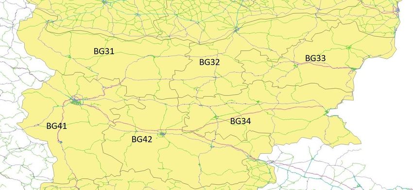
investments in less developed regions. The figures in Table 2 confirm this intuition: only 9% of the
BG41 imports come from the other Bulgarian regions, while the picture is different for the latter,
especially for BG31, BG32, and BG33 whose imports mostly come from the rest of Bulgaria, standing
at 65%, 50% and 44% of total imports, respectively.

One clear result arising from Table 10 is that TRNSP investments generate the largest spillovers of all,
suggesting that investing even in one sole region may affect the connectivity and quality of the
whole country’s transport network. Hence the spillover and the impact at the country-level should
be the largest when investing in regions hosting the main transport nodes and corridors of the
country regarding trade in goods and services. Figure 4 shows the road network of Bulgaria, from
which the central role played by the transport corridors of BG31, BG32 and BG42 in connecting the
country with its main trading partners emerges clearly. Given the fact that the trade partners of the
country such as Romania and Germany are located North-West, and Turkey and Greece in the South-
South-East, investments in BG31, BG32, and BG42 yield substantial returns for the country as a
whole, second only to those of BG41 investments (the latter generate high returns both for the large
trade flows characterising the region, and for its within-region activity).

Figure 4. Bulgaria road network

Source: PostGIS.

The above results lead to important policy considerations. If the objective of the policy is to foster
development in the less developed regions of Bulgaria and reduce regional disparities, investments
should take place there and not concentrate exclusively in the capital city region. Region-specific
returns may be the highest there, but they are mostly contained within the boundaries of the region
itself and the benefits would not trickle down to the other regions of the country.

On the contrary, given their high propensity to import from other regions within the country, the
impact of investments in less developed regions tends to spread to the whole country. For example,
investments in fields other than transport in BG31 and BG32 produce between 14 % and 24% of
their benefits outside the regions themselves, while in BG41 this share is at most 6% (and only 10%
for transport infrastructure). This argument is particularly prominent in fields of intervention such as
research and development, infrastructure and human capital. This implies that in order to maximise
the impact at country level, Cohesion Policy investments should not exclusively target the capital city
region. It also implies that there is no systematic efficiency-equity trade-off in Bulgaria as it is

possible to design policy portfolio which contribute to reduce regional disparities and at the same
time are conducive to a high impact at country level.

Another implication of the analysis is that the Cohesion Policy portfolio in less developed regions
should be balanced. Investments in infrastructure and transport are of course necessary in regions
where these resources may be lacking, but support to small and medium enterprises, to R&D and
investment in human capital remain key ingredients of a good development policy in these regions.
For instance, investments in R&D are sometimes believed to be better targeted at the most
developed regions only. This is probably relevant for frontier research activities, but R&D also covers
activities such as production processes and market and/or organisational innovation which are
relevant for economic agents in less developed regions as well.

4.3. Q2: What would be the impact of distributing half of the transport budget to the different
regions equally compared to the baseline situation?

It is not a priori clear whether reallocating transport investment from the more developed regions
(BG41 and BG42) receiving relatively larger amounts of TRNSP funds to the other regions would yield
a higher, lower or negligible GDP impact in Bulgaria. This would ultimately depend on the differences
in multipliers and intensity of the spillovers caused by the redistribution of funding.

Table 12 tabulates the redistribution of funding allocated to transport. We collect half of the budget
allocated to each region according to the baseline scenario and equally redistribute it to the six
regions. This alternative distribution of funds lead to additional TRNSP investments in BG31, BG32,
BG33, and BG34, while less money is allocated to BG41 and BG42.
Table 12. Baseline and Q2 alternative budgets allocated to transport infrastructure investments (€ mln)
 BG31 BG32 BG33 BG34 BG41 BG42 Total
TRNSP baseline 147.76 149.65 164.31 181.68 362.31 252.69 1,258.40*
Q2 alternative TRNSP scenario 178.75 179.69 187.02 195.71 286.02 231.21 1,258.40*
Source: JRC-DG REGIO calculations. * Corresponds to about 12% of the 2021-2027 Cohesion funding.

To identify which funding distribution generates the highest aggregate impact, we perform two
simulations. The first is a scenario in which we shock all regions only with the TRNSP investments of
the baseline scenario. The second is the alternative scenario reported in Table 12. In both cases the
investment is simultaneously deployed to all regions.

Figure 5 presents the cumulated GDP impact 20 years after the initial deployment of investment
(2040). The cumulated GDP impact per region is measured as the percentage difference from the
GDP of the no policy scenario.

Figure 5. Cumulated GDP impact in 2040, % difference with respect to the no policy scenario - Baseline vs Q2 TRNSP
 3.5

 3

 2.5

 2
 Baseline
 1.5 Q2 TRNSP

 1

 0.5

 0
 BG31 BG32 BG33 BG34 BG41 BG42 BG

Source: RHOMOLO simulations.

The GDP impact is larger in regions receiving additional funding, while it is smaller in BG41 and BG42
in which the investments were decreased under the alternative case than in the baseline scenario.
This is true both at the end of the implementation period (year 10 - not reported for brevity), when
the impact is mainly driven by the demand-side effects of the investments, and 20 years after the
beginning of the policy, a period in which supply-side effects are the main components of the policy
impact. For Bulgaria as a whole, the 20-year cumulated GDP impact is slightly higher in the
alternative scenario, although the difference can be considered negligible (+1.91% vs +1.93%).

Figure 6 shows the associated GDP multipliers under the two scenarios in 2040. The increase in the
multiplier for BG41 is particularly significant and it can be attributed to two different effects. First,
concentrating more of transport investment in other Bulgarian regions increases the spillovers from
which the capital city region benefits. In particular, the scenario implies that investments are larger
in BG31 and BG32, two regions crossed by important international trade corridors which partly
compensates for less investment in the more developed regions. Building transport infrastructures
there is therefore likely to generate substantial spillovers in BG41.

Second, investment in transport infrastructure feature decreasing returns to scale. Consequently, in
a region such as BG41 with a relatively large endowment, smaller investments tend to be more
productive than larger ones, making the multiplier higher under this scenario. As a result, even if
resources are shifted away from the capital city region where the returns are high, the impact per
euro at country level is hardly affected. At the same time, it contributes to reduce regional
disparities in the country.

Figure 6. Multipliers in 2040 - Baseline vs Q2 TRNSP
 1.4

 1.2

 1

 0.8
 Baseline
 0.6 Q2 TRNSP

 0.4

 0.2

 0
 BG31 BG32 BG33 BG34 BG41 BG42 BG

Source: RHOMOLO simulations.

Thus, even if investments in transport generate important spillovers since they affect the whole
transport network, in the case of Bulgaria, the regions benefitting from the transfer are also those
where the GDP impact tends to increase. Similarly, the impact decreases in the regions where
investments are reduced, and for the country as a whole there is hardly any significant difference in
terms of GDP impact between the two scenarios.

4.4. Q3: What would be the impact of distributing half of the energy efficiency budget to the
different regions equally compared to the current situation?

We follow the same strategy as in the previous section by generating an alternative distribution of
funding across regions, although in this case the focus is on infrastructure investments, which is how
energy efficiency spending is treated in RHOMOLO. Thus, we simulate solely the INFR investments
simultaneously deployed in all the regions of Bulgaria and we compare the resulting GDP impact and
multipliers with those of the baseline INFR investments.

Energy efficiency investments (SO 2.1: Promoting energy efficiency and reducing green-house gas
emissions) form part of the INFR field of intervention and are modelled in RHOMOLO as a public
investment shock IG increasing the stock of public capital. Table 13 shows the baseline distribution
and the alternative one related to the question above. In the latter case, similarly to the previous
section, half of the baseline initially allocated to each region is equally redistributed to the six
regions. This results in more investment being available in BG31, BG32, BG33, and BG34, and less in
BG41 and BG42, the latter two regions being the ones receiving the biggest shares of the total SO 2.1
budget in the baseline scenario.

Table 13. Baseline and Q3 alternative budget allocated to SO 2.1 (€ mln)
 BG31 BG32 BG33 BG34 BG41 BG42 Total
INFR baseline 34.71 35.15 38.59 42.67 85.10 59.35 295.56*
Q3 alternative INFR scenario 42,00 42.21 43.93 45.97 67.18 54.31 295.56*
Source: JRC-DG REGIO calculations. * Corresponds to about 3% of the 2021-2027 Cohesion funding.

Figure 7 shows the associated cumulated GDP impact (with respect to the no policy scenario) under
the two scenarios in 2040, ten years after the end of the implementation period. As in the previous
section, the results reveal that the GDP impact is larger in the regions receiving more investment
compared to the baseline, and smaller in the two regions in which investments decrease.10 The
effect of the shift of resources on the impact of the policy at country level is negligible, both at the
10 and 20-year intervals (the first is not reported for the sake of brevity).
Figure 7. Cumulated GDP impact in 2040, % difference with respect to the no policy scenario - Baseline vs Q3 INFR
 6

 5

 4

 3 Baseline
 Q3 INFR
 2

 1

 0
 BG31 BG32 BG33 BG34 BG41 BG42 BG

Source: RHOMOLO simulations.

The analysis of the multipliers (Figure 8) helps explaining why this redistribution of funds among
Bulgarian regions hardly affects the country-level impact of the policy on GDP.

The GDP multipliers in the two regions from which resources are shifted away are higher under the
Q3 INFR scenario. Similarly to the Q2 TRSNP scenario, this is due to a combination of higher positive
spillover from the regions where resources are transferred and to the decreasing returns to scale
attached to the accumulation of public capital. This implies that larger investments may be less
effective than smaller ones. This seems to be the case for BG41, since the amount invested in public
capital in the alternative scenario is significantly smaller than the one invested in the baseline
scenario, leading to a lower multiplier. As a result, even if resources are shifted away from the
regions where they are most productive, the increase in the multiplier generated in these regions is
such that the multiplier at the country level is only marginally affected.

10The effect of the shift continues to materialise for several years after the termination of the programmes since the public
capital stock is assumed to depreciate slowly, at a rate of 5% per year.

Figure 8. Multipliers in 2040 - Baseline vs Q3 INFR
 6

 5

 4

 3 Baseline
 Q3 INFR
 2

 1

 0
 BG31 BG32 BG33 BG34 BG41 BG42 BG

Source: RHOMOLO simulations.

In conclusion, shifting energy efficiency investments from more to less developed regions yields a
lower policy impact in the former and a higher impact in the latter. Since the impact on national GDP
is practically unchanged, the outcome promotes the mitigation of regional disparities without loss of
impact at country level.

4.5. Q4: What would be the impact of significantly increasing the transport or energy efficiency
allocation for the two least developed regions?

According to Table 1, the two least developed regions of Bulgaria are Severozapaden (Northwestern
- BG31) and Severen tsentralen (Northern Central - BG32), with a GDP per head corresponding
respectively to 33.1% and 35.5% of the EU average. In order to answer the question, we create two
alternative scenarios by shifting 20% of the funding allocated to each of these two regions to either
TRNSP or INFR. The total regional amount remains unchanged and resources are shifted towards
TRNSP or INFR from the other fields of intervention in proportion to their weight in the baseline
policy mix as shown in Table 14.

Table 14. Baseline and Q4 alternative policy portfolios (€ mln and % over total)

 Baseline Q4 TRNSP Q4 INFR
 FoI BG31 BG32 BG31 BG32 BG31 BG32

 RTD 79.6 (6.2%) 80.6 (6.2%) 77.5 (6.1%) 78.5 (6.1%) 64.0 (5%) 64.8 (5%)
 AIS 79.6 (6.2%) 80.6 (6.2%) 77.5 (6.1%) 78.5 (6.1%) 64.0 (5%) 64.8 (5%)
 INFR 633.6 (49.5%) 641.7 (49.5%) 617.0 (48.2% 624.9 (48.2%) 760.3 (59.4%) 770.0 (59.4%)
 TRNSP 147.8 (11.6%) 149.7 (11.6%) 177.3 (13.9%) 179.6 (13.9%) 118.8 (9.3%) 120.3 (9.3%)
 HC 295.9 (23.1%) 299.7 (23.1%) 288.2 (22.5%) 291.9 (22.5%) 237.8 (18.6%) 240.9 (18.6%)
 TA 42.8 (3.3%) 43.4 (3.3%) 41.7 (3.3%) 42.3 (3.3%) 34.4 (2.7%) 34.9 (2.7%)
 Total* 1,279.3 1,295.7 1,279.3 1,295.7 1,279.3 1,295.7
Source: DG REGIO. * Totals correspond to about 12% of the 2021-2027 Cohesion funding.

Figures 9 and 10 present the RHOMOLO simulation results, by comparing the impact on GDP 20
years after the start of the implementation period of TRNSP and INFR investments. These are
compared against the baseline case and are all expressed relative the GDP level of the no policy
scenario. Focusing on transport, the impact on GDP in the two least developed regions of the
country is slightly lower while there is no significant difference in impact in the other regions or at
the country level. Because the long run multiplier is relatively low for investments in transport
infrastructure in those regions (see Table 9), the shift of resources to this field away from the others
tends to reduce the policy impact. The consequences on the other regions and on the country as a
whole are negligible.
Figure 9. GDP impact in 2040, % difference with respect to the no policy scenario - Baseline vs Q4 TRNSP
 4.00

 3.50

 3.00

 2.50

 2.00 Baseline
 Q4 TRNSP
 1.50

 1.00

 0.50

 0.00
 BG31 BG32 BG33 BG34 BG41 BG42 BG

Source: RHOMOLO simulations.

On the contrary, the shift of the policy portfolio towards investment in energy efficiency increases
the GDP impact in the two regions concerned. Given the high INFR multipliers (see Table 9), an
increase in energy efficiency investment yields a slightly more effective policy portfolio. The effect of
this shift on the other regions is negligible while the impact at country level slightly increases.