A systems-based approach to parameterise seismic hazard in regions with little historical or instrumental seismicity: active fault and seismogenic ...
←
→
Page content transcription
If your browser does not render page correctly, please read the page content below
Solid Earth, 12, 187–217, 2021
https://doi.org/10.5194/se-12-187-2021
© Author(s) 2021. This work is distributed under
the Creative Commons Attribution 4.0 License.

A systems-based approach to parameterise seismic hazard
in regions with little historical or instrumental seismicity:
active fault and seismogenic source databases for
southern Malawi
Jack N. Williams1 , Hassan Mdala2 , Åke Fagereng1 , Luke N. J. Wedmore3 , Juliet Biggs3 , Zuze Dulanya4 ,
Patrick Chindandali5 , and Felix Mphepo2
1 School of Earth and Environmental Sciences, Cardiff University, Cardiff, UK
2 Geological Survey Department, Mzuzu Regional Office, Mzuzu, Malawi
3 School of Earth Sciences, University of Bristol, Bristol, UK
4 Geography and Earth Sciences Department, University of Malawi, Zomba, Malawi
5 Geological Survey Department, Zomba, Malawi

Correspondence: Jack N. Williams (williamsj132@cardiff.ac.uk)

Received: 5 June 2020 – Discussion started: 14 July 2020
Revised: 19 October 2020 – Accepted: 18 November 2020 – Published: 27 January 2021

Abstract. Seismic hazard is commonly characterised us-            timates ∼ 0.05–0.8 mm/yr) imply long recurrence intervals
ing instrumental seismic records. However, these records are      between events: 102 –105 years for border faults and 103 –
short relative to earthquake repeat times, and extrapolating to   106 years for intra-basin faults. Sensitivity analysis indicates
estimate seismic hazard can misrepresent the probable loca-       that the large range of these estimates can best be reduced
tion, magnitude, and frequency of future large earthquakes.       with improved geodetic constraints in southern Malawi. The
Although paleoseismology can address this challenge, this         SMAFD and SMSSD provide a framework for using geolog-
approach requires certain geomorphic setting, is resource in-     ical and geodetic information to characterise seismic hazard
tensive, and can carry large inherent uncertainties. Here, we     in regions with few on-fault slip rate measurements, and they
outline how fault slip rates and recurrence intervals can be      could be adapted for use elsewhere in the East African Rift
estimated by combining fault geometry, earthquake-scaling         and globally.
relationships, geodetically derived regional strain rates, and
geological constraints of regional strain distribution. We ap-
ply this approach to southern Malawi, near the southern
end of the East African Rift, and where, although no on-          1   Introduction
fault slip rate measurements exist, there are constraints on
strain partitioning between border and intra-basin faults. This   Earthquake ruptures tend to occur on pre-existing faults
has led to the development of the South Malawi Active             (Brace and Byerlee, 1966; Jackson, 2001; Scholz, 2002; Sib-
Fault Database (SMAFD), a geographical database of 23 ac-         son, 1989). Thus, the identification and systematic mapping
tive fault traces, and the South Malawi Seismogenic Source        of active faults, which are then compiled with other fault at-
Database (SMSSD), in which we apply our systems-based             tributes (e.g. slip rate and slip sense) into a geospatial active
approach to estimate earthquake magnitudes and recurrence         fault database, provide an important tool for assessing re-
intervals for the faults compiled in the SMAFD. We esti-          gional seismic hazard (Christophersen et al., 2015; Hart and
mate earthquake magnitudes of MW 5.4–7.2 for individual           Bryant, 1999; Langridge et al., 2016; Shyu et al., 2016; Sty-
fault sections in the SMSSD and MW 5.6–7.8 for whole-             ron et al., 2020; Styron and Pagani, 2020; Taylor and Yin,
fault ruptures. However, low fault slip rates (intermediate es-   2009). Not only can these databases provide information on

Published by Copernicus Publications on behalf of the European Geosciences Union.
188                                         J. N. Williams et al.: A systems-based approach to parameterise seismic hazard

the surface rupture risk (Hart and Bryant, 1999; Villamor et       where the instrumental record is relatively short compared
al., 2012), they can also be converted into earthquake sources     with fault recurrence intervals and where earthquakes may be
for probabilistic seismic hazard analysis (PSHA) to forecast       especially damaging (England and Jackson, 2011). It would
future levels of ground shaking (Beauval et al., 2018; Cor-        not, however, be appropriate for low-strain intraplate settings
nell, 1968; Gerstenberger et al., 2020; Hodge et al., 2015;        where geodetic data cannot resolve deformation rates (Calais
Morell et al., 2020; Stirling et al., 2012). Furthermore, the      et al., 2016),
data contained in active fault databases are inherently useful        By applying this approach to southern Malawi, we have
for understanding regional geological evolution (Agostini et       developed the South Malawi Seismogenic Source Database
al., 2011b; Basili et al., 2008; Taylor and Yin, 2009).            (SMSSD), which is a complementary database to the
   Active fault databases with worldwide coverage have been        SMAFD but where the attributes (e.g. fault segmentation,
compiled (Christophersen et al., 2015; Yeats, 2012), includ-       earthquake recurrence intervals) are (1) targeted towards its
ing recent development of the Global Earthquake Model              inclusion in PSHA and (2) derived from modelling (and are
Foundation Global Active Fault Database (Styron and Pa-            therefore mutable). Notably, previous PSHA in the EARS
gani, 2020). However, in some regions, the fault mapping in        has typically been conducted using the ∼ 65-year-long in-
these databases has only been performed at a coarse scale,         strumental seismic record alone (Ayele, 2017; Goitom et al.,
and the fault attributes (e.g. slip rates, earthquake recurrence   2017; Midzi et al., 1999; Poggi et al., 2017). However, fault-
intervals) that are required to use them as earthquake sources     based earthquake sources, such as the SMSSD, may play an
in PSHA have not been measured. This partly reflects that          important role in characterising the EARS’s ever-increasing
obtaining these attributes from dating faulted surfaces and/or     seismic risk (Goda et al., 2016; Hodge et al., 2015).
paleoseismology is time-intensive, requires certain geomor-           We describe the SMAFD and SMSSD together here so that
phic settings, and can involve large uncertainties (Cowie et       the assumptions and uncertainties of our approach are clear,
al., 2012; McCalpin, 2009; Nicol et al., 2016b). Alterna-          particularly for hazard modellers who may wish to incorpo-
tively, decadal timescale fault slip rates can be estimated us-    rate these databases into a PSHA. This study first describes
ing geodetic data and block models where the crust is di-          the seismotectonic setting of southern Malawi (Sect. 2),
vided by mapped faults (e.g. Field et al., 2014; Wallace et        and the approach used for mapping its active faults in the
al., 2012; Zeng and Shen, 2014). However, not all fault sys-       SMAFD (Sect. 3). In Sect. 4, we then describe the method
tems are covered by sufficiently dense geodetic networks to        used to estimate fault slip rates, earthquake magnitudes,
perform this analysis, the resulting slip rates may be biased      and recurrence intervals, and whose application to south-
by the short time over which these data have been collected        ern Malawi has resulted in the development of the SMSSD.
relative to earthquake cycles, and/or sometimes geodetic data      The SMAFD is described in Sect. 5 along with an evalua-
cannot resolve how strain is distributed (Calais et al., 2016;     tion of fault slip rate estimates and sensitivity analysis in the
Morell et al., 2020; Stein et al., 2012).                          SMSSD. Finally, in Sect. 6, we discuss the implication of
   In this study, we first describe the South Malawi Active        these databases in terms of southern Malawi’s seismic haz-
Fault Database (SMAFD), which is a systematic attempt to           ard, and the strategies needed to reduce uncertainties in these
map active faults and collate their geomorphic attributes in       databases.
southern Malawi. Located within the East African Rift Sys-
tem (EARS), southern Malawi lies in a region specifically
highlighted by Styron and Pagani (2020) as a priority area         2   Southern Malawi seismotectonics
for future active fault mapping; population growth in this re-
                                                                   The SMAFD and SMSSD cover the geopolitical term “south-
gion as well as seismically vulnerable building stock is also
                                                                   ern Malawi”; thus, they include all active faults between
driving an increased exposure to seismic hazard (Tectonic
                                                                   the southern end of Lake Malawi and the border between
Shift RIFT2018 Report, 2019; Goda et al., 2016; Hodge et
                                                                   Mozambique and Malawi. Faults that lie close to or cross
al., 2015; Kloukinas et al., 2020; Ngoma et al., 2019; Novelli
                                                                   this national boundary are also included. The extent of these
et al., 2019).
                                                                   databases does not therefore correspond directly to the geo-
   Within southern Malawi itself, faults capable of hosting
                                                                   logical region of the “southern Malawi Rift”, whose defini-
MW 7–8 earthquakes have been previously identified (Hodge
                                                                   tion has varied in previous studies (Chapola and Kaphwiyo,
et al., 2019, 2020; Jackson and Blenkinsop, 1997; Wedmore
                                                                   1992; Ebinger et al., 1987; Laõ-Dávila et al., 2015; Williams
et al., 2020a). However, there are currently no reports of his-
                                                                   et al., 2019). In this section, we briefly summarise the tec-
torical surface-rupturing earthquakes, on-fault slip rate mea-
                                                                   tonic history and seismic record in the region.
surements, or paleoseismic investigations. Thus, in the sec-
ond part of this study, we describe a new systems-based ap-
proach for combining geodetic and geological information
to estimate slip rates and earthquake recurrence intervals. In
particular, it may be useful for low-slip-rate interplate re-
gions (regional slip rates ∼ 1–10 mm/yr; Scholz et al., 1986)

Solid Earth, 12, 187–217, 2021                                                          https://doi.org/10.5194/se-12-187-2021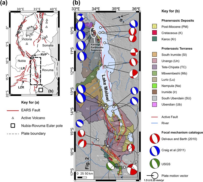
J. N. Williams et al.: A systems-based approach to parameterise seismic hazard                                                             189

Figure 1. (a) The location of Malawi in the context of major faults in the East African Rift (Daly et al., 2020; Hodge et al., 2018a; Macgregor,
2015) and plate boundaries proposed by Saria et al. (2013). LZR represents the Lower Zambezi Rift, LR represents the Luangwa Rift, and
RVP represents the Rungwe Volcanic Province. (b) A simplified geological map of Malawi, with Proterozoic terranes after Fullgraf et
al. (2017). The map is underlain by the Shuttle Radar Topography Mission (SRTM) 30 m digital elevation model (DEM; Sandwell et al.,
2011). The extent of Fig. 2 is also shown. Active faults within this area are those included in the South Malawi Active Fault Database
(SMAFD). Active faults outside this region are mapped as in panel (a). Focal mechanisms collated from Delvaux and Barth (2010), Craig et
al. (2011), and the U.S. Department of the Interior U.S. Geological Survey (2018). Minimum principal compressive stress (σ3 ) trend from
focal mechanism stress inversion (Williams et al., 2019). Plate motion vector for central point of each basin in southern Malawi (Fig. S1) for
the Nubia–Rovuma Euler pole (Saria et al., 2013), modelled using methods described in Robertson et al. (2016).

2.1   Southern Malawi tectonic setting                                    initiated prior to the mid-Pliocene (∼ 4.5 Ma) onset of sedi-
                                                                          ment accumulation in Lake Malawi’s south basin (Delvaux,
Southern Malawi lies towards the southern incipient end of                1995; McCartney and Scholz, 2016; Scholz et al., 2020) and
the EARS Western Branch, where it channels the Shire River                almost certainly not before the Oligocene (23–25 Ma) age of
from Lake Malawi to its confluence with the Zambezi River                 the Rungwe Volcanic Province (RVP) in southern Tanzania
(Dulanya, 2017; Ivory et al., 2016). This portion of the EARS             (Mesko, 2020; Mortimer et al., 2016; Roberts et al., 2012).
is typically considered to represent the divergent boundary               The RVP, 700 km to the north (Fig. 1a), marks the closest sur-
between the Rovuma and Nubia plates (Fig. 1a; Saria et al.,               face volcanism to southern Malawi; hence, this rift section is
2013; Stamps et al., 2008, 2018, 2020). However, recent seis-             considered to be amagmatic.
motectonic analysis suggests that the Nubia Plate can be fur-                Like elsewhere in the Western Branch, the EARS in south-
ther divided by the Lower Zambezi and Luangwa rifts into                  ern Malawi follows Proterozoic orogenic belts and can be di-
the San and Angoni plates, with the EARS in Malawi form-                  vided along strike into a number of 50–150 km long linked
ing the Angoni–Rovuma plate boundary (Fig. 1a; Daly et al.,               basins (Ebinger, 1989). Immediately south of Lake Malawi,
2020). EARS activity in southern Malawi is unlikely to have               the EARS bifurcates around the Shire Horst within the NW–

https://doi.org/10.5194/se-12-187-2021                                                                     Solid Earth, 12, 187–217, 2021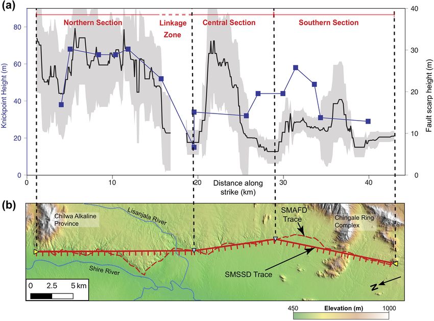
190                                             J. N. Williams et al.: A systems-based approach to parameterise seismic hazard

Figure 2. (a) Global Earthquake Model Global Active Fault Database map for southern Malawi (GAF-DB; Macgregor, 2015; Styron and
Pagani, 2020). The sub-Saharan African Global Earthquake Model (SSA-GEM; Poggi et al., 2017) event locations are also shown. (b) Map
of active fault traces compiled in the South Malawi Active Fault Database (SMAFD) with field locations and TanDEM-X coverage. Faults
not interpreted to be active are also shown. (c) Aeromagnetic image created from the vertical derivative, with foliation orientations digitised
from geological maps (Bloomfield, 1958, 1965; Bloomfield and Garson, 1965; Habgood et al., 1973; Walshaw, 1965). SMAFD faults shown
in white and the outline of lakes are shown by dashed white lines. For full details of the acquisition of the aeromagnetic data, see Laõ-Dávila
et al. (2015). (d) Simplified geometry of faults in the South Malawi Seismogenic Source Database (SMSSD), with faults sorted into border
and intra-basin faults. Ticks indicate fault hanging wall. The extent of all maps is equivalent and is outlined in Fig. 1b. All maps are underlain
by the SRTM 30 m digital elevation model. “Mal” denotes Malawi, and “Moz” denotes Mozambique.

Solid Earth, 12, 187–217, 2021                                                                     https://doi.org/10.5194/se-12-187-2021
J. N. Williams et al.: A systems-based approach to parameterise seismic hazard                                                191

SE trending Makanjira Graben before following an arcuate          1987) that are velocity weakening at temperatures < 700 ◦ C
bend in regional Proterozoic fabrics to form the NNE–SSW          (Hellebrekers et al., 2019) have been proposed as explana-
trending Zomba Graben (Fig. 2; Dulanya, 2017; Fullgraf et         tions for this unusually deep seismicity.
al., 2017; Laõ-Dávila et al., 2015; Wedmore et al., 2020a;           Earthquake focal mechanism stress inversions that encom-
Williams et al., 2019). Along strike to the south, the EARS       pass events from across Malawi indicate a normal fault stress
then intersects the Lower Shire Basin, a reactivated Karoo-       state (i.e. vertical maximum principal compressive stress)
age (i.e. Permo-Triassic) basin (Castaing, 1991; Chisenga et      with an ENE–WSW to E–W trending minimum principal
al., 2019; Habgood, 1963; Habgood et al., 1973; Wedmore           compressive stress (σ3 , Fig. 1b; Delvaux and Barth, 2010;
et al., 2020b), before bending around the Nsanje Horst to         Ebinger et al., 2019; Williams et al., 2019). This σ3 orienta-
link up with the Urema Graben in Mozambique (Bloom-               tion is comparable to the σ3 direction inferred from regional
field, 1958; Steinbruch, 2010). Daly et al. (2020) proposed       joint orientations (Williams et al., 2019) and the geodetically
that the Lower Shire Basin also extends to the west along         derived extension direction between the Nubia and Rovuma
the Mwanza Basin into Mozambique where it links with the          plates (Fig. 1b; Saria et al., 2014; Stamps et al., 2018, 2020).
Lower Zambezi Rift and forms the San–Angoni plate bound-             Using instrumental catalogues, probabilistic seismic haz-
ary (Fig. 1a).                                                    ard analysis (PSHA) finds that there is a 10 % probability
   Prior to this study, the only systematic active fault map-     of exceeding 0.15 g peak ground acceleration in the next
ping in southern Malawi had been conducted by Chapola and         50 years in southern Malawi (Midzi et al., 1999; Poggi et al.,
Kaphwiyo (1992) and, for the Lower Shire Basin, by Cas-           2017). Through the SMAFD and SMSSD, we outline how
taing (1991). These maps were subsequently incorporated           geological and geodetic data can be collated and assessed so
by Macgregor (2015) into EARS-scale maps, and later into          that they may also be incorporated into PSHA in southern
the Global Earthquake Model Global Active Fault Database          Malawi.
(Styron and Pagani, 2020). However, the faults are mapped
at a coarse scale (Fig. 2a), and this database does not in-
clude active faults traces identified in legacy geological maps   3     Mapping and describing active faults in the South
(Bloomfield, 1965; Bloomfield and Garson, 1965; Habgood                 Malawi Active Fault Database (SMAFD)
et al., 1973; Walshaw, 1965) and high-resolution digital el-
evation models (Hodge et al., 2019, 2020; Wedmore et al.,         An active fault database consists of an active fault map,
2020a, b).                                                        where for each fault, attributes are added that detail geomor-
                                                                  phic, kinematic, geometric, and geological information about
2.2   Southern Malawi seismicity                                  the fault (Christophersen et al., 2015; Styron and Pagani,
                                                                  2020). Typically, an active fault database is stored in a geo-
There are no known historical accounts of surface-rupturing       graphic information system (GIS) environment, in which the
earthquakes in southern Malawi, although a continuous writ-       fault attributes are assigned to a linear feature that represents
ten record only extends to ca. 1870 (Pike, 1965; Stahl, 2010).    the fault’s geomorphic trace (e.g. Langridge et al., 2016; Ma-
However, in northern Malawi, the previously unrecognised          chette et al., 2004; Styron et al., 2020). In this section, we
St Mary Fault exhibited surface rupture following the 2009        describe how active faults were mapped in the South Malawi
Karonga earthquakes, a sequence consisting primarily of four      Active Fault Database (SMAFD) as well as the geomorphic
shallow (focal depths < 8 km) MW 5.5–5.9 events over a 13 d       attributes that were assigned to them. Estimates of associ-
period (Fig. 1b; Biggs et al., 2010; Gaherty et al., 2019;        ated earthquake source parameters, which are collated sep-
Hamiel et al., 2012; Kolawole et al., 2018b; Macheyeki et         arately in the South Malawi Seismogenic Source Database
al., 2015).                                                       (SMSSD), are described in Sect. 4.
   The International Seismological Centre (ISC) record for
Malawi is complete from 1965 to present for events with           3.1    Identifying active and inactive faults in southern
MW > 4.5 (Figs. 1b, 2a; Hodge et al., 2015), with the largest            Malawi
event in this record being the 1989 MW 6.3 Salima earth-
quake (Jackson and Blenkinsop, 1993). Notably, seismicity         There are many inherent limitations in mapping active faults.
in Malawi is commonly observed to depths far greater (30–         Even in countries with well-developed databases, such as
35 km; Craig et al., 2011; Delvaux and Barth, 2010; Jackson       Italy and New Zealand, their success in accurately predict-
and Blenkinsop, 1993) than would be expected for continen-        ing the locations of future surface-rupturing earthquakes is,
tal crust of typical composition and geothermal gradient (10–     at best, mixed (Basili et al., 2008; Nicol et al., 2016a). An ac-
15 km). Thick cold anhydrous lower crust (Craig et al., 2011;     tive fault might not be recognised because evidence of previ-
Jackson and Blenkinsop, 1997; Njinju et al., 2019; Nyblade        ous surface rupture is subsequently buried, eroded (Wallace,
and Langston, 1995), localised weak viscous zones embed-          1980), or the fault itself is blind (e.g. Quigley et al., 2012),
ded within strong lower crust (Fagereng, 2013), and/or vol-       which in turn depends on earthquake magnitude, focal depth,
umes of mafic material in the lower crust (Shudofsky et al.,      thickness of the seismogenic crust, and the local geology.

https://doi.org/10.5194/se-12-187-2021                                                          Solid Earth, 12, 187–217, 2021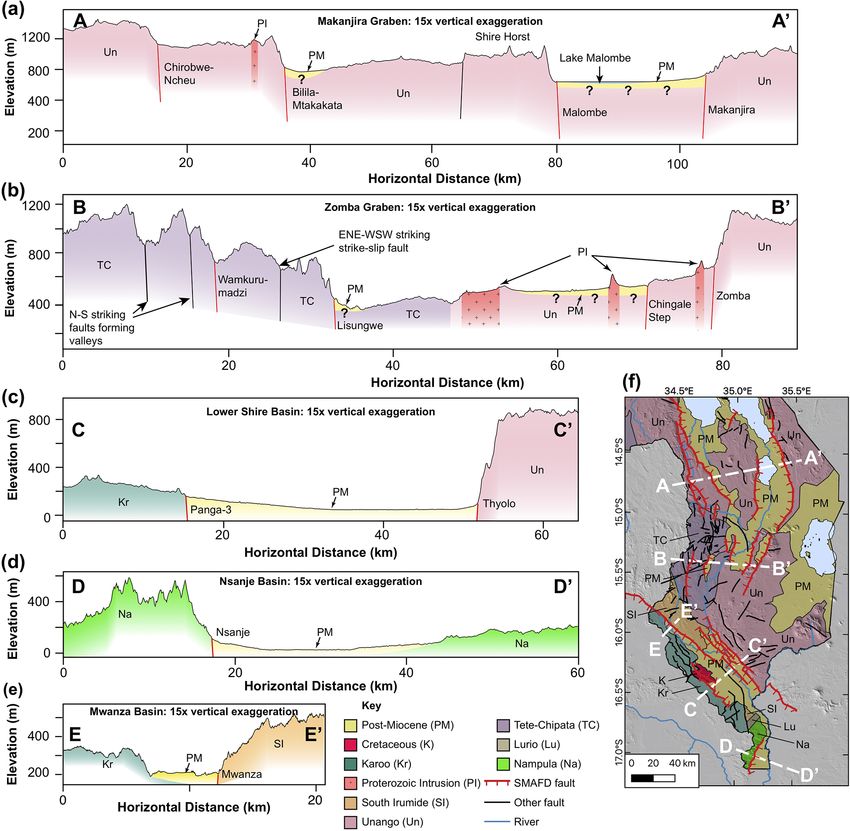
192                                           J. N. Williams et al.: A systems-based approach to parameterise seismic hazard

Furthermore, although active and inactive faults are typically        (Fig. 2a). However, this map is not necessarily complete for
differentiated by the age of the most recent earthquake, the          all other faults in southern Malawi, and we also cannot defini-
precise maximum age that is used to define “active” varies            tively exclude the possibility that some of these faults are still
between different active fault databases depending on the re-         active although they display no evidence for it. The relatively
gional strain rate (i.e. plate boundary vs. stable craton) and        broad definition of an active fault may also mean that some
the prevalence of youthful sediments (Clark et al., 2012; Jo-         inactive faults are included in the SMAFD. However, in ap-
mard et al., 2017; Langridge et al., 2016; Machette et al.,           plying the opposite approach (i.e. requiring an absolute age
2004). Indeed, it may not always be possible to reliably de-          for the most recent activity on a fault) there is a greater risk
termine if an exposed fault has been recently active or not           that faults mistakenly interpreted to be inactive subsequently
(Cox et al., 2012; Nicol et al., 2016a).                              rupture in a future earthquake (Litchfield et al., 2018; Nicol
   Each of these issues has relevance to mapping active               et al., 2016a).
faults in southern Malawi. Firstly, active faults may be
buried by sediments deposited due to tectonic subsidence              3.2     Datasets for mapping faults in southern Malawi
(Gawthorpe and Leeder, 2000) and/or by regular (10–100 ka)
climate-driven ∼ 100 m scale fluctuations in the level of Lake        3.2.1    Legacy geological maps
Malawi, which would likely flood the Zomba and Makan-
                                                                      Between the 1950s and 1970s, the geology of southern
jira basins (Ivory et al., 2016; Lyons et al., 2015; Wed-
                                                                      Malawi was systematically mapped at a 1 : 100 000 scale.
more et al., 2020a). Alternatively, the relatively thick (30–
                                                                      These studies noted evidence of recent displacement on the
35 km) seismogenic crust in southern Malawi means that
                                                                      Thyolo (Habgood et al., 1973), Bilila–Mtakataka, Tsikulam-
even moderate–large earthquakes (MW > 6) do not neces-
                                                                      owa (Walshaw, 1965), and Mankanjira faults (King and Daw-
sarily result in surface rupture, as illustrated by the MW 6.3
                                                                      son, 1976). However, they did not systematically distinguish
Salima earthquake (Gupta, 1992; Jackson and Blenkinsop,
                                                                      between active and inactive faults. Furthermore, these stud-
1993). Finally, except for studies around Lake Malombe (Van
                                                                      ies are in places ambiguous with equivalent structures in the
Bocxlaer et al., 2012), there is no chronostratigraphic control
                                                                      Zomba Graben being variably described as “terrace features”
for this section of the EARS to help differentiate between
                                                                      (Bloomfield, 1965), active fault scarps (Dixey, 1926), and
inactive and active faults (Dulanya, 2017; Wedmore et al.,
                                                                      Late Jurassic–Early Cretaceous faults (Dixey, 1938).
2020a).
   Thus, for the SMAFD, we define active faults based on
                                                                      3.2.2    Geophysical datasets
evidence of activity within the current tectonic regime. Such
an approach has been advocated elsewhere in the EARS                  Regional-scale aeromagnetic data were acquired across
(Delvaux et al., 2017) and in other areas with low levels of          Malawi in 2013 by the Geological Survey Department of
seismicity, few paleoseismic studies, and/or where there are          Malawi (Fig. 2c; Kolawole et al., 2018a; Laõ-Dávila et al.,
faults that are favourably oriented for failure in the current        2015). These survey data were used to refine fault mapping
stress regime but that have no definitive evidence of recent          in cases where features interpreted as faults in the aeromag-
activity (Nicol et al., 2016a; De Pascale et al., 2017; Vil-          netic survey extended beyond their surface expression. Grav-
lamor et al., 2018). In practice, this means that faults will be      ity surveys have also been used to map blind faults in the
included in the SMAFD if they can be demonstrated to have             Lower Shire Basin (Chisenga et al., 2019), and these have
been active during East African rifting. This evidence can            been incorporated into the SMAFD.
vary from the accumulation of post-Miocene hanging-wall
sediments to the presence of a steep fault scarp, offset allu-        3.2.3    Digital elevation models
vial fans, and/or knickpoints in rivers that have migrated only
a short vertical distance (< 100 m) upstream (Hodge et al.,           The topography of southern Malawi is primarily controlled
2019, 2020; Jackson and Blenkinsop, 1997; Wedmore et al.,             by EARS faulting (Dulanya, 2017; Laõ-Dávila et al., 2015;
2020a). We note that the absence of post-Miocene sediments            Wedmore et al., 2020a) except in the case of the Kirk Range
in the hanging wall of a normal fault does not necessarily im-        (Fig. 2b) as well as readily identifiable igneous intrusions
ply that it is inactive, if, for example, faults are closely spaced   and Karoo faults (Figs. 3c, 4b). To exploit this interaction
across strike so that sediments are eroded during subsequent          between topography and active faulting, TanDEM-X digital
footwall uplift of an interior normal fault (e.g. Chirobwe–           elevation models (DEMs) with a 12.5 m horizontal resolu-
Ncheu Fault, Fig. 3c; see also Mortimer et al., 2016; Muir-           tion and an absolute vertical mean error of ±0.2 m (Wessel
head et al., 2016). In these cases, if there is other evidence of     et al., 2018) were acquired for southern Malawi (Fig. 2b).
recent activity (e.g. scarp, triangular facets), these faults are     This small error means that the TanDEM-X data perform bet-
still included.                                                       ter at identifying the metre-scale scarps common in south-
   For the sake of completeness, major faults that control            ern Malawi (Hodge et al., 2019; Wedmore et al., 2020a)
modern-day topography but that do not fit the criteria of             than the more widely used but lower-resolution Shuttle Radar
being active (e.g. Karoo faults) were mapped separately               Topography Mission (SRTM) 30 m DEMs (Sandwell et al.,

Solid Earth, 12, 187–217, 2021                                                             https://doi.org/10.5194/se-12-187-2021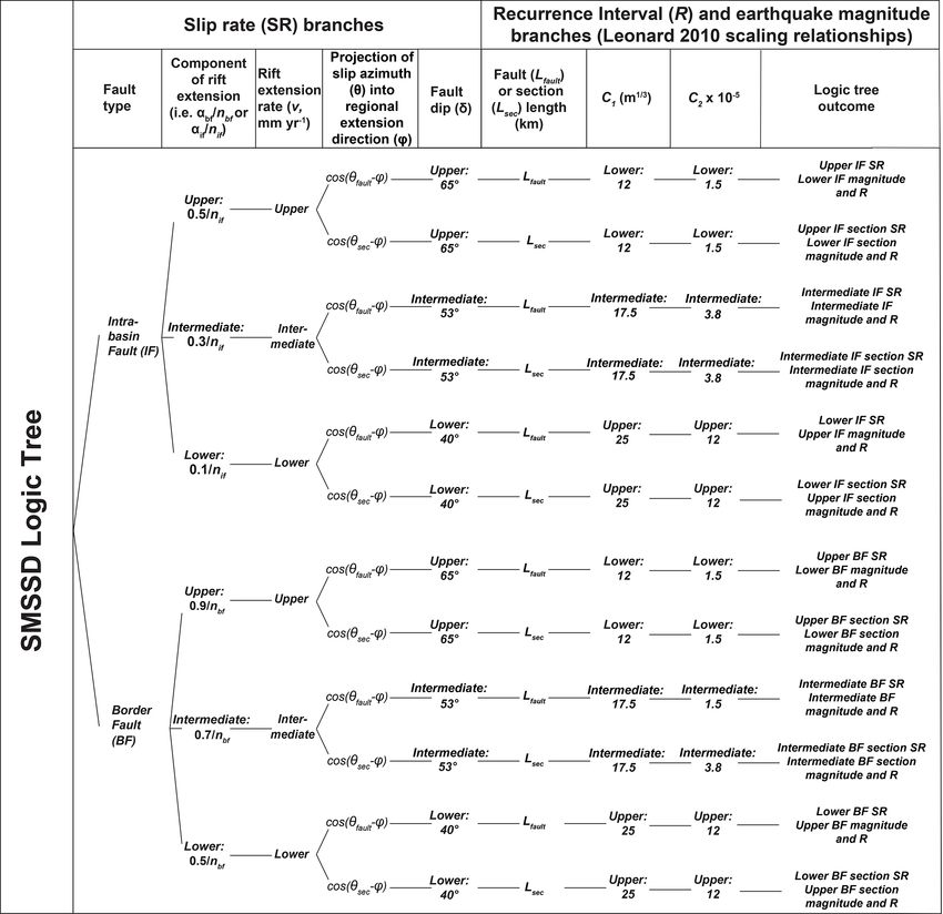
J. N. Williams et al.: A systems-based approach to parameterise seismic hazard 193
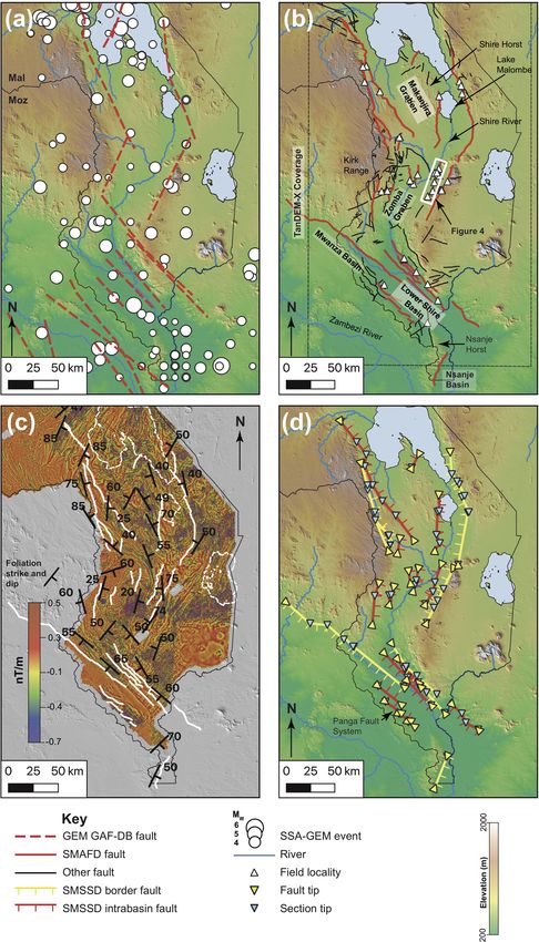
Figure 3. Field examples of border and intra-basin faults in southern Malawi. Unmanned aerial vehicle (UAV) images of scarps (dashed
red line) along the (a) intra-basin Mlungusi Fault in the Zomba Graben as well as (b) the Thyolo Fault – the border fault for the Lower
Shire Basin. (c) View across the western edge of the Makanjira Graben showing the Chirobwe–Ncheu and Bilila–Mtakataka faults as well as
Proterozoic syenite intrusions (Walshaw, 1965). (d) Minor step in the scarp along the intra-basin Chingale Step fault, with the escarpment of
the Zomba border fault behind.
2011). Furthermore, TanDEM-X data can be used to assess 3.2.4 Fieldwork
variations in along-strike scarp height (Hodge et al., 2018a,
2019; Wedmore et al., 2020a, b) and the interactions be- To corroborate evidence of recent faulting recognised in
tween footwall uplift and fluvial incision (Fig. 4a; Wedmore DEMs and geological reports, fieldwork was conducted on
et al., 2020a). The Mwanza and Nsanje faults partly extended several faults (Fig. 2b). This ranged from documenting fea-
out of the region of TanDEM-X coverage, and these sec- tures indicative of recent displacement on the faults, such
tions were mapped using the SRTM 30 m resolution DEM as scarps, triangular facets, and displaced Quaternary–recent
(Fig. 2b). sediments, to comprehensively sampling the fault and sur-
veying it with an unmanned aerial vehicle (Fig. 3; see also:
Hodge et al., 2018a; Wedmore et al., 2020a, b; Williams et
al., 2019).
https://doi.org/10.5194/se-12-187-2021 Solid Earth, 12, 187–217, 2021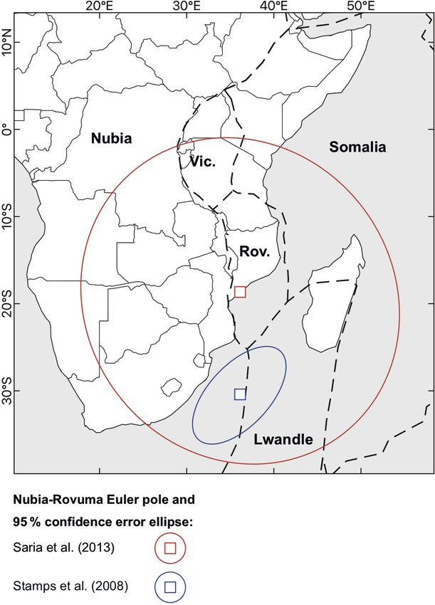
194 J. N. Williams et al.: A systems-based approach to parameterise seismic hazard
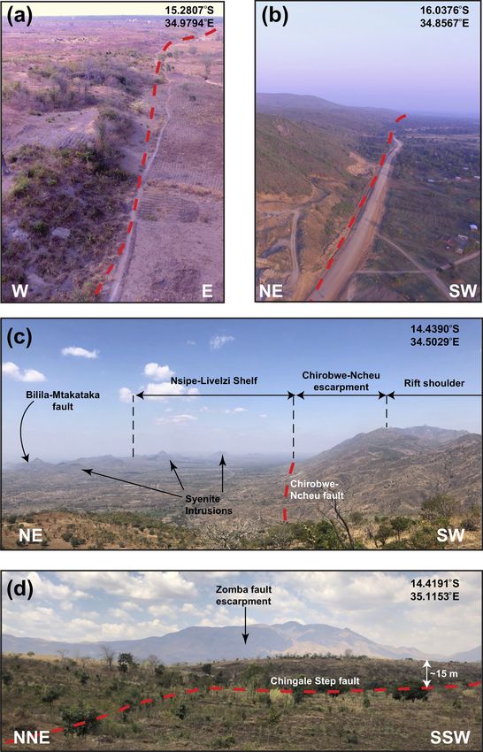
Figure 4. Fault segmentation along the Chingale Step fault, modified after Wedmore et al. (2020a). (a) Along-strike variation in stream
knickpoint (blue points) and fault scarp height (black line), with the gap due to erosion by the Lisanjala River. Grey shading represents
1 standard deviation error in scarp height measurements (Wedmore et al., 2020a). (b) A map of the Chingale Step fault underlain by TanDEM-
X DEM, with the extent of the area shown in Fig. 2b. The dashed red line shows the surface trace of the fault as per the South Malawi Active
Fault Database (SMAFD). The solid red line shows the simplified geometry of the fault in the South Malawi Seismogenic Source Database
(SMSSD), where it is defined by straight lines between section end points (blue triangles). Ticks indicate fault hanging wall. An along-strike
scarp height minima at the boundary between the northern and central section occurs at a bend in the fault scarp; however, there is no obvious
geometrical complexity at the along-strike scarp height minima between the southern and central sections. Topography associated with the
Proterozoic Chingale Ring Structure and Chilwa Alkaline Province (Bloomfield, 1965; Manda et al., 2019) is also indicated. For full details
on panel (a), see Wedmore et al. (2020a).
3.3 Strategy for mapping and describing active faults fault was mapped (Table 1). Some fault attributes used in
in the SMAFD the GEM GAF-DB, such as slip rates, are not included in
the SMAFD, as these data have not been collected in south-
Following the active fault definition and synthesis of the ern Malawi. We instead derive these attributes as outlined in
datasets described above, faults in southern Malawi are Sect. 4 and incorporate them separately into the SMSSD (Ta-
mapped following the approach outlined for the Global ble 2). However, within each database, a numerical ID system
Earthquake Model Global Active Fault Database (GAF-DB) is used make the two databases compatible (Tables 1, 2).
where each fault constitutes a single continuous GIS feature
(Styron and Pagani, 2020). Therefore, the SMAFD differs
from other active fault databases where each distinct geomor- 4 A systems-based approach to estimating seismic
phic (i.e. traces) or geometric (i.e. sections) part of a fault source parameters: application to southern Malawi
is mapped as a separate GIS feature (Christophersen et al.,
2015; Machette et al., 2004). Typically, estimates of fault slip rate, earthquake magnitudes,
The attributes associated with each fault in the SMAFD are and recurrence intervals are derived from paleoseismology,
listed and briefly described in Table 1. These resemble the at- geodesy, historical records of past earthquakes, or considera-
tributes in the GEM GAF-DB that describe a fault’s geomor- tions of the seismic moment rate (Basili et al., 2008; Field et
phic attributes and confidence that it is still active (Styron and al., 2014; Langridge et al., 2016; McCalpin, 2009; Molnar,
Pagani, 2020). To incorporate the multidisciplinary approach 1979; Youngs and Coppersmith, 1985). However, as noted
that we have used to map faults in southern Malawi, we also in Sect. 1, these types of data have not been collected in
include a “Location method” attribute, which details how the southern Malawi. Indeed, very few such records currently
Solid Earth, 12, 187–217, 2021 https://doi.org/10.5194/se-12-187-2021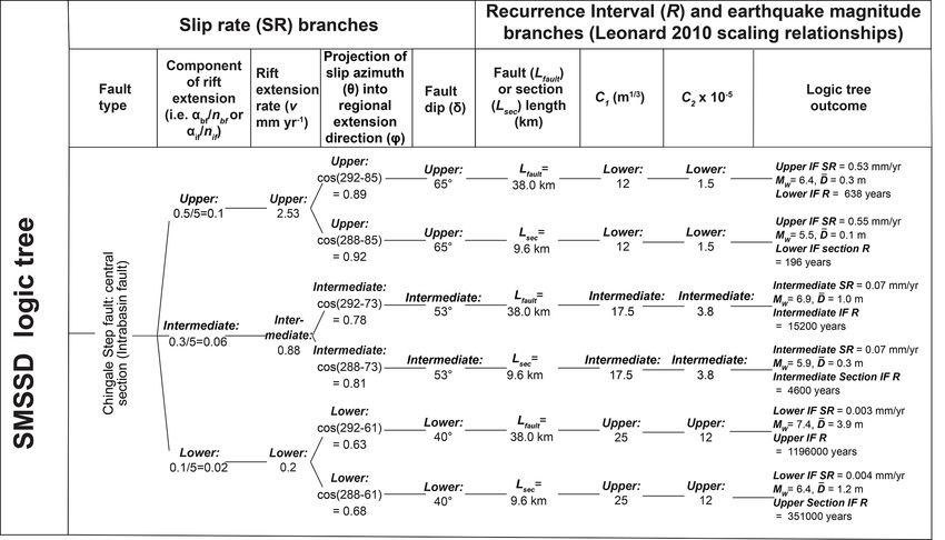
J. N. Williams et al.: A systems-based approach to parameterise seismic hazard                                                     195

Table 1. List and brief description of attributes in the SMAFD. Attributes are based on the Global Earthquake Model Global Active Faults
Database (Styron and Pagani, 2020).

           Attribute                  Type                 Description                         Notes
           SMAFD-ID                   Numeric, assigned    Unique two-digit numerical
                                                           reference ID for each trace
           Name                       Text                                                     Assigned based on previous
                                                                                               mapping or local geographic
                                                                                               feature.
           Geomorphic expression      Text                 Geomorphological feature used       For example, scarp and escarp-
                                                           to identify and map fault trace.    ment
           Location method            Text                 Dataset used to map trace.          For example, type of digital el-
                                                                                               evation
                                                                                               model
           Accuracy                   Numeric, assigned    Coarsest scale at which trace       Reflects the prominence of the
                                                           can be mapped; expressed as         fault’s geomorphic expression.
                                                           denominator of map scale.
           activity_confidence        Numeric, assigned    Certainty of neotectonic            1 if certain, 2 if uncertain
                                                           activity
           exposure_quality           Numeric, assigned    Fault exposure quality              1 if high, 2 if low
           epistemic_quality          Numeric, assigned    Certainty that fault exists there   1 if high, 2 if low
           last_movement              Text                                                     Currently this is unknown for
                                                                                               all faults in southern Malawi
                                                                                               but can be updated when new
                                                                                               information becomes available.
           References                 Text                 Relevant geological maps/
                                                           literature where fault has
                                                           been previously described.
           SMSSD ID                   Numeric, assigned    ID of equivalent structure in       Will be multiple IDs for multi-
                                                           South Malawi Seismogenic            segment faults, as these consist
                                                           Source Database                     of multiple potential earthquake
                                                                                               sources

exist across the entire EARS (Delvaux et al., 2017; Muir-              practice elsewhere, be explored with a logic tree approach
head et al., 2016; Siegburg et al., 2020; Zielke and Strecker,         (Fig. 6; Field et al., 2014; Vallage and Bollinger, 2019; Vil-
2009), and even in regions with well-developed active fault            lamor et al., 2018). We use the South Malawi Seismogenic
databases, such as California and New Zealand, only a small            Source Database (SMSSD) as an example of how this ap-
number of faults have directly measured slip rates and pa-             proach can be applied to narrow (< 100 km width; Buck,
leoseismic information (Field et al., 2014; Langridge et al.,          1991) amagmatic continental rifts, where the distribution of
2016).                                                                 regional strain between border faults and intra-basin faults is
   In the absence of direct on-fault slip rate estimates, we           well constrained by previous studies (Agostini et al., 2011a;
suggest that they can be estimated through a systems-level             Corti, 2012; Gupta et al., 1998; Morley, 1988; Muirhead et
approach in which geodetically derived plate motion rates              al., 2016, 2019; Nicol et al., 1997; Shillington et al., 2020;
are partitioned across faults in a manner consistent with their        Wedmore et al., 2020a; Wright et al., 2020).
geomorphology and regional tectonic regime. Although such
an approach has been used before over small regions (Cox               4.1    Earthquake source geometry
et al., 2012; Litchfield et al., 2014), it has not been ap-
plied to an entire fault system. In addition, we outline how           Faults may rupture both along their entire length and in
the uncertainties and alternative hypotheses that are inher-           smaller individual-section ruptures that are often bounded by
ent to this approach can, in common with seismic hazard                changes in fault geometry (DuRoss et al., 2016; Goda et al.,
                                                                       2018; Gómez-Vasconcelos et al., 2018; Hodge et al., 2015;

https://doi.org/10.5194/se-12-187-2021                                                                 Solid Earth, 12, 187–217, 2021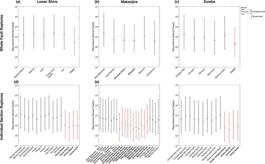
196                                           J. N. Williams et al.: A systems-based approach to parameterise seismic hazard

Table 2. List and brief description of fault geometry, slip rate estimates, and earthquake source attributes in the SMSSD.

      Attribute                 Type           Description                                 Notes
      SMSSD-ID                  Numeric,       Unique numerical reference ID for
                                assigned       each seismic source
      Fault name                Text           Fault that section belongs to               Assigned based on previous mapping or local
                                                                                           geographic feature.
      Section name              Text                                                       Assigned based on previous mapping, local
                                                                                           geographic feature, or location along fault.
      Basin                     Text           Basin that fault is located within.         Used in slip rate calculations.
      Fault type                Text           Intra-basin or border fault
      Section length            Numeric,       Straight-line distance between              Measured in kilometres. Except for linking sec-
      (Lsec )                   assigned       section tips.                               tions, must be > 5 km.
      Section strike            Numeric,       Measured from section tips, using
                                assigned       bearing that is < 180◦ .
      Fault length              Numeric,       Straight-line distance between fault        Measured in kilometres.
      (Lfault )                 assigned       tips or sum of Lsec for segmented faults.
      Fault strike              Numeric,       Measured from fault tips using              For segmented (i.e. non-planar) this is an “aver-
                                assigned       bearing < 180◦ .                            aged” value of fault geometry, which is required
                                                                                           for slip rate estimates (Eq. 3).
      Dip (δ)                   Numeric,                                                   Attribute parameterised by a set of representa-
                                assigned                                                   tive values (40, 53, 65◦ ).
      Dip direction             Text           Compass quadrant that fault dips in.
      Fault width (W )          Numeric,       Calculated from Eq. (2) from                Not equivalent to rupture width for individual-
                                calculated     Leonard (2010) scaling                      section earthquakes.
                                               relationship using Lfault .
      Slip type                 Text           Fault kinematics                            All faults in the SMSSD assumed to be normal
      Section net slip          Numeric,       Calculated from Eq. (3).                    In millimetres per year. All faults in the SMSSD
      rate                      calculated                                                 assumed to be normal, so is equivalent to dip-
                                                                                           slip rate.
      Fault net slip rate       Numeric,       Calculated from Eq. (3).                    In millimetres per year. All faults in the SMSSD
                                calculated                                                 assumed to be normal, so is equivalent to dip-
                                                                                           slip rate. Different from section net slip rate
                                                                                           where fault strike 6 = section strike.
      Section earthquake        Numeric,       Calculated from Leonard (2010) scaling      Lower, intermediate, and upper values
      magnitude                 calculated     relationship using Eq. (4) and Lsec .       calculated.
      Fault earthquake          Numeric,       Calculated from Leonard (2010) scaling      Lower, intermediate, and upper values
      magnitude                 calculated     relationship using Eq. (4) and Lfault .     calculated.
      Section earthquake        Numeric,       Calculated from Eq. (6) and using Lsec      Lower, intermediate, and upper values
      recurrence interval (R)   calculated     to calculate average single-event           calculated.
                                               displacement in Eq. (5).
      Fault earthquake          Numeric,       Calculated from Eq. (6) and using Lfault    Lower, intermediate, and upper values
      recurrence interval (R)   calculated     to calculate average single-event           calculated.
                                               displacement in Eq. (5).
      Fault notes               Text           Remaining miscellaneous information
                                               about fault.
      References                Text           Relevant geological maps/literature
                                               where fault has been
                                               previously described.
      SMAFD-ID                  Numeric,       ID of equivalent structure in South
                                assigned       Malawi Active Fault Database

Solid Earth, 12, 187–217, 2021                                                                  https://doi.org/10.5194/se-12-187-2021
J. N. Williams et al.: A systems-based approach to parameterise seismic hazard 197
Iezzi et al., 2019; Valentini et al., 2020). Therefore, the ba- seismic reflection data (Mortimer et al., 2007; Wheeler and
sic GIS feature in the SMSSD is a fault section, where in- Rosendahl, 1994), and aeromagnetic surveys (Kolawole et
dividual faults from the SMAFD may be divided into multi- al., 2018a) elsewhere in Malawi.
ple sections by bends in their fault trace (Fig. 2d; DuRoss It is typically assumed that fault width (W ) can be esti-
et al., 2016; Jackson and White, 1989; Wesnousky, 2008; mated by projecting the difference in lower and upper seis-
Zhang et al., 1991). Along-strike minima in fault displace- mogenic depth into fault dip (δ), with the assumption that
ment (e.g. scarp or knickpoint height) may also be indicative faults are equidimensional up to the point where W is limited
of segmentation (Willemse, 1997), but these do not always by the thickness of the seismogenic crust (Christophersen et
coincide with geometrical complexities in southern Malawi al., 2015):
(Fig. 4; Hodge et al., 2018a, 2019; Wedmore et al., 2020a, b).
Lfault , where Lfault ≤ sinz δ ;
This may indicate that deeper structures, not visible in the W= (1)
z z
surficial fault geometry, are also influencing fault segmenta- sin δ , where Lfault > sin δ
tion (Wedmore et al., 2020b). Therefore, where along-strike
In southern Malawi, both seismogenic thickness, z (30–
scarp height measurements exist, these local minima are also
35 km; Jackson and Blenkinsop, 1993; Craig et al., 2011),
used to define fault sections (Figs. 2d, 4).
and δ (40–65◦ , as justified above) are poorly constrained, so a
Faults that are closely spaced across strike but are not
range of W values must be considered. Furthermore, ruptures
physically connected may also rupture together through “soft
unlimited by z are not necessarily equidimensional (Leonard,
linkages” (Childs et al., 1995; Wesnousky, 2008; Willemse,
2010; Wesnousky, 2008). Therefore, in the SMSSD, we esti-
1997; Zhang et al., 1991). In the SMSSD, we follow em-
mate W from an empirical scaling relationship between fault
pirical observations and Coulomb stress modelling that sug-
length and W (Leonard, 2010):
gests that normal fault earthquakes may rupture across steps
whose width is < 20 % of the combined length of the inter- β
W = C1 Lfault , (2)
acting sections, up to a maximum separation of 10 km (Biasi
and Wesnousky, 2016; Hodge et al., 2018b), and we use this where Lfault > 5 km, and C1 and β are empirically derived
as a criteria to assign whether two en echelon faults in the constants that are equal to 17.5 and 0.66 respectively for in-
SMSSD may rupture together. terplate dip-slip earthquakes (Leonard, 2010). As shown in
A number of geometrical attributes are then assigned to Fig. 5c, when applying Eq. (2), estimates of W in the SMSSD
both individual sections and whole faults in the SMSSD (Ta- are consistent with (1) observations of > 1 length-to-width
ble 2). Section length (Lsec ) is defined as the straight-line ratios for dip-slip earthquakes (Fig. 5c) and (2) the thick seis-
distance between section end points (Fig. 4b). This approach mogenic crust in East Africa (i.e. W ∼ 40 km, Fig. 5c; Craig
avoids the difficulty of measuring the length of fractal fea- et al., 2011; Ebinger et al., 2019; Jackson and Blenkinsop,
tures, and it accounts for the hypothesis that small-scale 1993; Lavayssière et al., 2019; Nyblade and Langston, 1995).
(less than kilometre-scale) variations in fault geometry in
southern Malawi may represent only near-surface complex- 4.2 Estimating fault slip rates
ity (depths < 5 km) and that the faults are relatively planar
at depth (Hodge et al., 2018a). However, it only provides a For a narrow amagmatic continental rift such as the EARS
minimum estimate of section length. For segmented faults in in southern Malawi, the first step to estimate slip rates is to
the SMSSD, fault length (Lfault ) is the sum of Lsec , other- divide the rift along its axis into its basins (Fig. 2b); within
wise Lfault is the distance between its tips (Fig. 4b). As each each basin, the mapped faults are then divided into border
GIS feature in the SMSSD represents a distinct earthquake and intra-basin faults. We define border faults geometrically,
source, we consider that Lsec and/or Lfault must be > ∼ 5 km, as a fault located at the edge of the rift with the implicit as-
except in the case of linking sections that rupture only in sumption that all other mapped active faults are intra-basin
whole-fault ruptures. (Christophersen et al., 2015). faults (Fig. 2d; Ebinger, 1989; Gawthorpe and Leeder, 2000;
In southern Malawi, fault dip is either unknown or uncer- Muirhead et al., 2019; Wedmore et al., 2020b). These geo-
tain, because fault planes are rarely exposed, surface pro- metric definitions have no direct implications for how dis-
cesses affect scarp angle (Hodge et al., 2020), and/or dip at placement is partitioned among border and intra-basin faults.
depth is not constrained. This difficulty in measuring fault The slip rate for each fault or fault section i is then esti-
dip is common, and dip has been parameterised using a range mated using the following equation:
of reasonable values in these cases (Christophersen et al., (
αbf v cos(θ(i)−φ)
2015; Langridge et al., 2016; Styron et al., 2020). Thus, nbf cos δ , for border faults
Slip rate (i) = αif v cos(θ(i)−φ) (3)
we assign minimum, intermediate, and maximum dip val- nif cos δ , for intra-basin faults
ues in the SMSSD of 40, 53, and 65◦ respectively, which
encapsulate dip estimates from field data in southern Malawi Here, θ (i) is the fault or fault section slip azimuth, v and ϕ
(Hodge et al., 2018a; Williams et al., 2019), and earthquake are the respective horizontal rift extension rate and azimuth,
focal mechanisms (Biggs et al., 2010; Ebinger et al., 2019), α is a weighting applied to each fault depending on whether
https://doi.org/10.5194/se-12-187-2021 Solid Earth, 12, 187–217, 2021198 J. N. Williams et al.: A systems-based approach to parameterise seismic hazard
Figure 5. Assessment of fault geometry in the SMSSD. (a) Histograms showing the distribution of (a) fault (Lfault ) and section (Lsec )
lengths in the SMSSD. (b) Histogram of fault widths in the SMSSD as derived from the Leonard (2010) scaling relationship (Eq. 2); in
panel (c), the predicted aspect ratio of faults following this relationship (dashed grey line) in comparison to an alternative method to estimate
W using Eq. (1) (white circles). (d) A comparison of empirical scaling relationships used to estimate earthquake magnitudes (MW ) from
fault geometry in the SMSSD. Leonard (2010) magnitudes estimated using Eq. (4), with error bars representing range of C1 and C2 values
derived for interplate dip-slip faults. A is the fault area calculated from Lfault and W using Eq. (1), WC94 is from Wells and Coppersmith
(1994), and W08 is from Wesnousky (2008).
it is a border (αbf ) or intra-basin (αif ) fault, and it is divided wall flexure (Muirhead et al., 2016; Shillington et al., 2020),
by the number of mapped border faults (nbf ) or intra-basin lower crustal rheology (Heimpel and Olson, 1996; Wedmore
faults (nif ) in each basin (Fig. 6). Although Eq. (3) is specific et al., 2020a), and whether border faults have attained their
for rifts, it could be adapted in other tectonic settings where maximum theoretical displacement (Accardo et al., 2018;
there is an a priori understanding of the rate and distribution Olive et al., 2014; Scholz and Contreras, 1998). In some in-
of regional strain – for example, to distribute regional strain cipient rifts like southern Malawi, extensional strain is ob-
between the basal detachment and thrust ramps in a fold and served to be localised (∼ 80 %–90 %) on its border faults
thrust belt (Poblet and Lisle, 2011), to distribute regional (Muirhead et al., 2019; Wright et al., 2020). Furthermore,
strain between multiple subparallel faults in a strike-slip sys- evidence from boreholes and topography indicates that bor-
tem, or to assess more complex strain partitioning between der faults in southern Malawi have relatively small throws
kinematically distinct fault populations in transtensional or (< 1000 m, Fig. S1), which combined with its thick seis-
transpressional systems (Braun and Beaumont, 1995). mogenic crust indicates that the flexural extensional strain
The distribution of v between border (αbf ) and intra-basin on its intra-basin faults is likely to be negligible (Billings
faults (αif ) in an amagmatic narrow rift depends on factors and Kattenhorn, 2005; Muirhead et al., 2016; Wedmore et
such as total rift extension (Ebinger, 2005; Muirhead et al., al., 2020a). However, detailed analysis of fault scarp heights
2016, 2019), rift obliquity (Agostini et al., 2011b), hanging- across the Zomba Graben indicates that ∼ 50 % of exten-
Solid Earth, 12, 187–217, 2021 https://doi.org/10.5194/se-12-187-2021J. N. Williams et al.: A systems-based approach to parameterise seismic hazard 199 Figure 6. Logic tree for calculating lower, intermediate, and upper estimates of fault slip rates and earthquake magnitudes and recurrence intervals in the SMSSD; αbf and αif are the rift extension weighting assigned to border faults (BF) and intra-basin faults (IF) respectively; nbf and nif are the number of border or intra-basin faults in a basin respectively; and θfault and θsec are the respective whole-fault and individual-section slip azimuth values. sional strain is currently distributed onto its intra-basin faults 50 %, and 70 % between the Nsanje Fault and a border fault (Wedmore et al., 2020a). To account for this uncertainty identified 25 km along strike in Mozambique (Fig. S1; Mac- in the SMSSD, lower, intermediate, and upper estimates of gregor, 2015) to estimate its lower, intermediate, and upper αbf are set to 0.5, 0.7, and 0.9 respectively (Fig. 6). As slip rate. αif = 1 − αbf , respective lower, intermediate, and upper es- In the SMSSD, the horizontal extension rate, v, is taken timates are 0.1, 0.3, and 0.5 (Fig. 6). from the plate motion vector between the Rovuma and Nubia Where distinct intra-basin faults kinematically interact plates at the centre of each individual basin (Table 3, Figs. 1b, across steps, we consider these as one fault in Eq. (3), as this S1) using the Euler poles reported by Saria et al. (2013). We equation accounts for strain across, not along, the rift. For the use the Euler pole (as defined by a location and rotation rate) Mwanza and Nsanje basins, no intra-basin faults are identi- and the uncertainties associated with the Euler pole (defined fied (Fig. 2b), so all the extension strain is assigned to their by an error ellipse; Fig. A1) to calculate the plate motion and border faults (i.e. αbf = 1). In the case of the Nsanje Basin, the plate motion uncertainty between the Rovuma and Nubia however, this is extension is divided into increments of 30 %, plates for each basin (Table 3, Fig. 1b) following the methods https://doi.org/10.5194/se-12-187-2021 Solid Earth, 12, 187–217, 2021
200                                                 J. N. Williams et al.: A systems-based approach to parameterise seismic hazard

Table 3. Coordinates from which the Nubia–Rovuma plate motion vector for different basins in southern Malawi was derived (Fig. 1b). The
velocity, azimuth, and uncertainties of each vector are also reported given the Nubia–Rovuma Euler poles in Saria et al. (2013) (S13) or in
Stamps et al. (2008) (S08; Fig. A1) and where the uncertainties associated with the Euler pole are derived from the methods presented in
Robertson et al. (2016). For justification of basin centre locations, see Fig. S1.

               Basin                  Centre of basin   Centre of basin   Geodetic     Velocity and velocity   Azimuth, and azi-
                                         latitude (S)    longitude (E)    model         uncertainty of plate   muthal uncertainty
                                                                                            motion (mm/yr)       of plate motion
               Makanjira                       14.51             34.88    S13                   1.08 ± 1.66         075◦ ± 089◦
                                                                          S08                   3.01 ± 0.28         085◦ ± 002◦
               Zomba                           15.42             34.93    S13                   0.88 ± 1.65         072◦ ± 110◦
                                                                          S08                   2.84 ± 0.28         085◦ ± 002◦
               Lower Shire                     16.26             35.08    S13                   0.69 ± 1.65         069◦ ± 141◦
                                                                          S08                   2.69 ± 0.28         086◦ ± 002◦
               Nsanje                          17.28             35.23    S13                   0.46 ± 1.63         063◦ ± 212◦
                                                                          S08                   2.49 ± 0.27         086◦ ± 002◦
               Mwanza                            n/a               n/a    n/a                      0.6 ± 0.4                  n/a

             n/a: “not applicable”.

outlined in Robertson et al. (2016). With this approach, the                    fault are estimated with ϕ set to 061 and 085◦ respectively).
lower bound of v is negative (i.e. the plate motion is contrac-                 An example of these slip rate calculations for the central sec-
tional; Table 3). However, the topography and seismicity of                     tion of the Chingale Step fault is provided in Fig. 7.
southern Malawi clearly indicate that it is not a contractional
regime nor is it a stable craton. Therefore, a lower bound of                   4.3   Earthquake magnitudes and recurrence intervals
0.2 mm/yr horizontal extension is assigned in the SMSSD,
which is considered the minimum strain accrual that is mea-                     We estimate earthquake magnitudes in the SMSSD by apply-
surable using geodesy (Calais et al., 2016). There are no                       ing empirically derived scaling relationships between fault
geodetic constraints for the extension rate across the Mwanza                   length and earthquake magnitude. Scaling relationships be-
Basin as it lies along the poorly defined Angoni–San plate                      tween fault length and average single-event displacement
boundary (Daly et al., 2020). Therefore, we assign this basin                   (D) can then be combined with slip rate estimates to cal-
an extension rate of 0.2–1 mm/yr. This reflects the smaller                     culate earthquake recurrence intervals (R) through the re-
escarpment height along its border fault (250 m vs. ∼ 750 m;                    lationship R = D / slip rate (Wallace, 1970). To select an
Fig. 2b) relative to the Lower Shire Basin, which indicates a                   appropriate set of earthquake-scaling relationships for the
slower average extension rate over geological time.                             SMSSD, we consider three previously reported regressions
   The rift extension azimuth (ϕ) in southern Malawi is de-                     and apply them to its mapped faults: (1) between normal
rived from a regional focal mechanism stress (073◦ ± 012◦ ,                     fault length and MW (Wesnousky, 2008), (2) interplate dip-
Fig. 1b; Delvaux and Barth, 2010; Ebinger et al., 2019;                         slip fault length and MW (Leonard, 2010), and (3) fault area
Williams et al., 2019), as there is considerable uncertainty                    and MW (Wells and Coppersmith, 1994) where A is calcu-
in this parameter from geodesy (Table 3; Saria et al., 2013).                   lated using W derived from Eq. (1).
Faults in southern Malawi are considered to be normal (Del-                        We find that although generally comparable for MW < 7.5,
vaux and Barth, 2010; Hodge et al., 2015; Williams et al.,                      the Wells and Coppersmith (1994) regression overestimates
2019). Therefore, the slip azimuth (θ (i)) is the dip direction                 magnitudes relative to Leonard (2010) (Fig. 5d). This likely
of each fault or fault section, where it is then projected into                 reflects the discrepancy in W between applying Eq. (1) and
ϕ in Eq. (3). Although this sets up an apparent inconsistency                   the Leonard (2010) regression (Eq. 2; Fig. 5c; Sect. 4.1). The
in which variably striking faults accommodate normal dip-                       Wesnousky (2008) regression overestimates magnitudes for
slip under a uniform extension direction, this phenomena that                   MW < 6.9 relative to Leonard (2010) equations and underes-
can be explained by lateral heterogeneity in the lower crust                    timates them at larger magnitudes (Fig. 5d). This may reflect
in southern Malawi (Corti et al., 2013; Philippon et al., 2015;                 that the Wesnousky (2008) regression is derived from only
Wedmore et al., 2020a; Williams et al., 2019). To account                       six events, and these events show a poor correlation between
for the uncertainty in ϕ, upper and lower extension rates are                   length and MW (Pearson’s regression coefficient = 0.36).
obtained by varying ϕ ±012◦ depending on the fault’s dip di-                    Given these considerations, the Leonard (2010) regressions
rection (e.g. upper slip rate estimates for NE and NW dipping                   are used in the SMSSD. Furthermore, these regressions are

Solid Earth, 12, 187–217, 2021                                                                      https://doi.org/10.5194/se-12-187-2021
J. N. Williams et al.: A systems-based approach to parameterise seismic hazard 201
used to estimate W (Sect. 4.1) and are self-consistent when on its eastern edge, and three well-defined intra-basin fault
estimating MW and D from Lfault , which is not necessarily scarps in its interior (Fig. 8b; Bloomfield, 1965; Wedmore et
true for the other cases. al., 2020a). The western edge of the Zomba Graben grades
Thus, MW and D are estimated in the SMSSD by onto the Kirk Plateau where there are several deeply incised
N–S trending valleys that have been previously mapped as
MW (i) =
“rift valley faults” (Fig. 8b; Bloomfield and Garson, 1965).
5 3
2 log Lsec + 2 log C1 +log C2 µ −9.09
However, only one of these faults has an active scarp and
for individual-section ruptures and
1.5 (4) accumulated post-Miocene sediments (the Lisungwe Fault;
5
log Lfault + 32 log C1 +log C2 µ −9.09
2 Wedmore et al., 2020a). In addition, the Wamkurumadzi
for whole-fault ruptures, and
1.5
Fault, which lies to the west of the Lisungwe, is also in-
logD(i) = cluded in the SMAFD – albeit with low confidence – as
5 1
6 log Lsec + 2 log C1 + log C2 µ for individual-section ruptures and (5) evidence of recent activity is noted by Bloomfield and Gar-
5 1 son (1965), and any recent sediments may have been eroded
6 log Lfault + 2 log C1 + log C2 µ for whole-fault ruptures,
by the Wamkurumadzi River that flows along its base. Given
where µ is the shear modulus (3.3×10¹⁰ Pa), C1 is as defined the complex topography and ambiguity on fault activity, we
for Eq. (2), and C2 is another constant derived by Leonard tentatively interpret these faults as intra-basin faults in the
(2010). Both constants are varied between the full range of SMSSD and note that the western Zomba Graben should be
values derived in a least square analysis (Leonard, 2010) to a priority area for future fault mapping.
obtain lower, intermediate, and upper estimates of MW and The floor of the NW–SE trending Lower Shire Basin lies at
D (Figs. 6, 7). Following Eq. (5), recurrence intervals R(i) an elevation 350 m lower than the floor of the Zomba Graben.
can be calculated as follows: Between these two EARS sections basement is exposed, and
D(i) there is no evidence of tectonic activity that falls within the
R(i) = , (6) SMAFD definition of an active fault. Gravity surveys and to-
Slip rate(i)
pographic data indicate that the Lower Shire Basin exhibits
where upper estimates of R are calculated by dividing the a half-graben structure, with the Thyolo Fault bounding it
upper estimate of D by the lowest estimate of fault or sec- to the northeast (Fig. 8d; Chisenga et al., 2019; Wedmore et
tion slip rate and vice versa (Fig. 6). An example of these al., 2020b). A number of intra-basin faults have been iden-
earthquake source calculations for the central section of the tified in the hanging wall of the Thyolo Fault (Chisenga et
Chingale Step fault is provided in Fig. 7. al., 2019), although none are identified in the Nsanje and
Mwanza basins (Fig. 8d, e).
5 Key features of the SMAFD and SMSSD
5.2 Fault slip rates, and earthquake magnitudes and
In this section, we briefly describe the fault mapping collated recurrence intervals in the SMSSD
in the SMAFD and then the present fault slip rates, earth-
quake magnitudes, and recurrence intervals in the SMSSD By implementing a logic tree approach to assess uncertainty
as estimated by our systems-based approach. in the SMSSD, three values (lower, intermediate, and upper)
are derived for each calculated attribute (Table 2, Fig. 6).
5.1 Border and intra-basin faults in southern Malawi However, it is implicit that the upper and lower values have a
low probability as they require a unique, and possibly unreal-
The SMAFD contains 23 active faults across five EARS istic, combination of parameters. Therefore, we primarily re-
basins. The northernmost faults lie in the NW–SE trending port values obtained from applying the intermediate branches
Makanjira Graben, a full graben where two border faults, the in the logic tree but discuss the uncertainties in Sect. 5.4.
Makanjira and Chirobwe–Ncheu, clearly define either side of Although the SMAFD contains 23 active faults, these are
the rift (Fig. 8a). Four intra-basin faults are identified, with, further subdivided into 74 sections in the SMSSD – of which
two of them, the Bilila–Mtakataka and Malombe faults, ex- 13 are linking sections. Section lengths (Lsec ) range between
hibiting steep scarps (Hodge et al., 2018a, 2019). In particu- 0.7 and 62 km, whereas fault lengths (Lfault ) vary from 6.2 to
lar, one-dimensional diffusional models of scarp degradation 144 km (Fig. 5a, Table 4). The highest slip rates are estimated
suggest that the Bilila–Mtakataka Fault scarp formed within to be on the Thyolo and Zomba faults (intermediate estimates
the past 10 000 years (Hodge et al., 2020). The Malombe of 0.6–0.8 mm/yr). On intra-basin faults in the SMSSD, in-
Fault forms a ∼ 500 m high escarpment that bounds the Shire termediate slip rate estimates are 0.05–0.1 mm/yr (Fig. 9).
Horst and divides post-Miocene deposits in the Makanjira Slip rates tend to be relatively fast in the Makanjira Graben
Graben across strike (Fig. 8a; Hodge et al., 2019; Laõ-Dávila (Fig. 9c), as the extension rate is higher (Table 3), and its
et al., 2015). NNW–SSE striking faults are more optimally oriented to the
Along strike to the south, the NNE–SSW trending Zomba regional extension direction (Fig. 2). The difference between
Graben contains a prominent border fault, the Zomba Fault, upper and lower slip rate estimates in the SMSSD logic tree is
https://doi.org/10.5194/se-12-187-2021 Solid Earth, 12, 187–217, 2021You can also read