Accuracy assessment of global internal-tide models using satellite altimetry - Deep Blue
←
→
Page content transcription
If your browser does not render page correctly, please read the page content below
Ocean Sci., 17, 147–180, 2021
https://doi.org/10.5194/os-17-147-2021
© Author(s) 2021. This work is distributed under
the Creative Commons Attribution 4.0 License.

Accuracy assessment of global internal-tide models
using satellite altimetry
Loren Carrere1 , Brian K. Arbic2 , Brian Dushaw3 , Gary Egbert4 , Svetlana Erofeeva4 , Florent Lyard5 ,
Richard D. Ray6 , Clément Ubelmann7 , Edward Zaron8 , Zhongxiang Zhao9 , Jay F. Shriver10 ,
Maarten Cornelis Buijsman11 , and Nicolas Picot12
1 CLS,  Ramonville-Saint-Agne, 31450, France
2 Department  of Earth and Environmental Sciences, University of Michigan, Ann Arbor, MI, USA
3 independent researcher: Girona, 17004, Spain
4 Department Geology and Geophysics, Oregon State University, Corvallis, OR 97331-5503, USA
5 LEGOS-OMP laboratory, Toulouse, 31401, France
6 NASA Goddard Space Flight Center, Greenbelt, MD 20771, USA
7 Ocean Next, La Terrasse, 38660, France
8 Department of Civil and Environmental Engineering, Portland State University, Portland, OR 97207-0751, USA
9 Applied Physics Laboratory, University of Washington, Seattle, WA, USA
10 Naval Research Laboratory, Stennis Space Center, MS, USA
11 Division of Marine Science, University of Southern Mississippi, Stennis Space Center, MS 39529, USA
12 CNES, Toulouse, 31400, France

Correspondence: Loren Carrere (lcarrere@groupcls.com)

Received: 31 May 2020 – Discussion started: 23 June 2020
Revised: 17 September 2020 – Accepted: 19 October 2020 – Published: 19 January 2021

Abstract. Altimeter measurements are corrected for several       which represent an unprecedented and valuable global ocean
geophysical parameters in order to access ocean signals of in-   database. The internal-tide models presented here focus on
terest, like mesoscale or sub-mesoscale variability. The ocean   the coherent internal-tide signal and they are of three types:
tide is one of the most critical corrections due to the ampli-   empirical models based upon analysis of existing altimeter
tude of the tidal elevations and to the aliasing phenomena       missions, an assimilative model and a three-dimensional hy-
of high-frequency signals into the lower-frequency band, but     drodynamic model.
the internal-tide signatures at the ocean surface are not yet       A detailed comparison and validation of these internal-
corrected globally.                                              tide models is proposed using existing satellite altimeter
   Internal tides can have a signature of several centimeters    databases. The analysis focuses on the four main tidal con-
at the surface with wavelengths of about 50–250 km for the       stituents: M2 , K1 , O1 and S2 . The validation process is based
first mode and even smaller scales for higher-order modes.       on a statistical analysis of multi-mission altimetry including
The goals of the upcoming Surface Water Ocean Topogra-           Jason-2 and Cryosphere Satellite-2 data. The results show a
phy (SWOT) mission and other high-resolution ocean mea-          significant altimeter variance reduction when using internal-
surements make the correction of these small-scale signals a     tide corrections in all ocean regions where internal tides are
challenge, as the correction of all tidal variability becomes    generating or propagating. A complementary spectral anal-
mandatory to access accurate measurements of other oceanic       ysis also gives some estimation of the performance of each
signals.                                                         model as a function of wavelength and some insight into the
   In this context, several scientific teams are working on      residual non-stationary part of internal tides in the different
the development of new internal-tide models, taking advan-       regions of interest. This work led to the implementation of a
tage of the very long altimeter time series now available,

Published by Copernicus Publications on behalf of the European Geosciences Union.
148                                                     L. Carrere et al.: Accuracy assessment of global internal-tide models

new internal-tide correction (ZARON’one) in the next geo-           ocean measurements in general, removing these small-scale
physical data records version-F (GDR-F) standards.                  surface signals is a challenge because we need to be able to
                                                                    separate all tidal signals to access other oceanic variability of
                                                                    interest such as mesoscale, sub-mesoscale or climate signals.
1   Introduction                                                       A large part of the internal-tide signal remains coherent
                                                                    over long times, with large stable propagation patterns across
Since the early 1990s, several altimeter missions have been         ocean basins, such as the North Pacific and many other re-
monitoring sea level at a global scale, nowadays offering a         gions (Dushaw et al., 2011). The amplitude of the coher-
long and very accurate time series of measurements. This            ent signal appears to be greatly diminished in the equato-
altimetry database is nearly homogeneous over the entire            rial regions, which may be caused by the direct disrupting
ocean, allowing the sampling of many regions that were              effect of the rapid equatorial wave variations (Buijsman et
poorly sampled or not sampled at all before the satellite era.      al., 2017) or merely masked by the background noise. The
Thanks to its current accuracy and maturity, altimetry is now       seasonal variability of the ocean medium and the interaction
regarded as a fully operational observing system dedicated to       with mesoscale eddies and currents may also disrupt the co-
ocean and climate applications (Escudier et al., 2017).             herence of the internal tide in many other areas, which makes
   The main difficulty encountered when using altimeter             the non-coherent internal tides’ variability more complex to
datasets for ocean studies is related to the long revisit time of   observe and model (Shriver et al., 2014).
the satellites, which results in the aliasing of high-frequency        In this context, and since conventional satellite altimetry
ocean signals into a much lower-frequency band. Concern-            has already shown its ability to detect small-scale internal-
ing tidal frequencies, the 9.9156 d cycle of TOPEX/Poseidon         tide surface signatures (Ray and Mitchum, 1997; Dushaw
and Jason altimeter series induces the aliasing of the semidi-      2002; Carrere et al., 2004), several scientific teams have
urnal M2 lunar tide into a 62 d period, and the diurnal K1 tide     developed new internal-tide models, taking advantage of
is aliased into a 173 d period, the latter of which is very close   the very long altimeter time series now available. These
to the semiannual frequency and raises complex separation           internal-tide models are of three types: empirical models
problems. The long duration of the global ocean altimeter           based upon analysis of existing altimeter missions, usu-
database available has allowed the community to overcome            ally more than one; assimilative models based upon as-
this separation problem, and new global ocean barotropic            similating altimeter data into a reduced-gravity model; and
tidal solutions (Stammer et al., 2014) have been produced           three-dimensional hydrodynamic models, which embed in-
taking advantage of altimeter data: among them the last God-        ternal tides into an eddying general circulation model. In
dard/Grenoble Ocean Tide model (denoted GOT: Ray, 2013)             the present paper, the analysis is focused on seven models
and the last finite-element solution for ocean tide (denoted        that yield a coherent internal-tide solution: Dushaw (2015),
FES2014: Carrere et al., 2016a; Lyard et al., 2020), which          Egbert and Erofeeva (2014), Ray and Zaron (2016), Shriver
are commonly used as reference for the barotropic tide cor-         et al. (2014), Clément Ubelmann (personal communication,
rection in actual altimeter geophysical data records (denoted       2017), Zaron (2019), and Zhao et al. (2016, 2019a).
GDRs). Moreover this altimeter database has been used in               The objective of this paper is to present a detailed compari-
numerous studies to validate new instrumental and geophys-          son and a validation assessment of these internal-tide models
ical corrections used in altimetry, thanks to the analysis of       using satellite altimetry. The present analysis focuses on the
their impact on the sea level estimation at climate scales, as      coherent internal-tide signal for the main tidal constituents:
well as at lower temporal scales like mesoscale signals; in         M2 , S2 , K1 and O1 . The validation process is based on a sta-
particular, it has proven its efficiency for validating global      tistical analysis and on a comparison to multi-mission altime-
ocean models (Shum 1997; Stammer et al., 2014; Carrere et           try including Jason-2 (denoted J2 hereafter) and Cryosphere
al., 2016b; Quartly et al., 2017).                                  Satellite-2 (also named CryoSat-2 or C2 hereafter) LRM data
   The upcoming Surface Water Ocean Topography (SWOT)               (low-resolution mode). For the sake of clarity, only results
mission, led by NASA, CNES, and the UK and Canadian                 for the main tidal components M2 and K1 are presented in
space agencies, is planned for 2021 and will measure sea sur-       the core of this paper, and O1 and S2 validation results are
face height with a spatial resolution never proposed before,        gathered in the Appendix.
thus raising the importance of the correction of the internal-         After a brief description of the participating models
tide surface signature. Internal tides (denoted ITs) are gener-     (Sect. 2), an analysis of the differences between internal-tide
ated by an incoming barotropic tidal flow on a bathymetric          models is presented in Sect. 3. Section 4 describes the altime-
pattern within a stratified ocean and can have amplitudes of        ter dataset used, the method of comparison and the valida-
several tens of meters at the thermocline level and a signa-        tion strategy. The validation results of the different internal-
ture of several centimeters at the surface, with wavelengths        tide corrections versus altimetry databases are described in
ranging approximately between 30 and 250 km for the low-            Sects. 5 and 6. Finally, a discussion and concluding remarks
est three modes of variability (Chelton et al., 1998). From         are gathered in Sect. 7.
the perspective of the SWOT mission and of high-resolution

Ocean Sci., 17, 147–180, 2021                                                            https://doi.org/10.5194/os-17-147-2021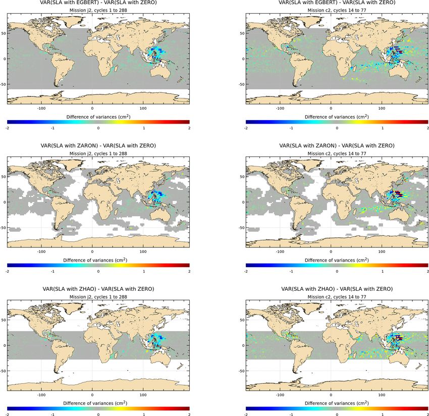
L. Carrere et al.: Accuracy assessment of global internal-tide models                                                           149

2     Presentation of participating internal-tide models            times discontinuous within these overlapping zones. For this
                                                                    study, global maps of the harmonic constants for the two
This section gives a brief overview of the internal-tide mod-       first baroclinic modes of the largest semidiurnal tidal con-
els evaluated in this study. We considered five purely em-          stituent M2 were computed on a regular 1/20◦ grid (Dushaw,
pirical models involving data merging, one data assimilative        2015; the complete solution is available from http://www.
model and also one pure hydrodynamic model simulating               apl.washington.edu/project/project.php?id=tm_1-15, last ac-
tides and internal tides using the gravitational forcing and a      cess: 17 December 2020). This global M2 solution was tested
high spatial resolution but without any internal-tide data con-     against pointwise, along-track estimates for the internal tide,
straint. The list of participating IT models is given in Table 1.   with satisfactory comparisons in the Atlantic and Pacific
                                                                    oceans. Comparisons were also made to in situ measure-
2.1    Empirical models                                             ments by ocean acoustic tomography in the Pacific and At-
                                                                    lantic, showing a good predictability in both amplitude and
The purely empirical models are based upon the analysis of          phase. By comparisons to the tomography data, internal tides
existing conventional altimeter missions, usually more than         within the Philippine Sea (Dushaw, 2015) or Canary Basin
one. The five empirical models used in the present study are        (Dushaw et al., 2017) were less predictable. Some of these
briefly described below.                                            comparisons found good agreement between hindcasts and
                                                                    time series recorded in the western North Atlantic about a
DUSHAW                                                              decade before the altimetry data were available, which is con-
                                                                    sistent with the extraordinary temporal coherence of this IT
This global model was computed using a frequency–                   signal in many regions of the world’s oceans.
wavenumber tidal analysis (Dushaw et al., 2011; Dushaw,
2015). The internal tides were assumed to be composed of            RAY
narrow-band spectra of traveling waves, and these waves are
fitted to the altimeter data in both time and position. A tidal     The RAY model provides a global chart of surface eleva-
analysis of a time series allows extracting accurate tidal es-      tions associated with the stationary M2 internal-tide sig-
timates from noisy or irregular data under the assumptions          nal. This map is empirically constructed from multi-mission
that the signal is temporally coherent and described by a           satellite altimeter data, including GFO (GEOSAT Follow-
few known frequencies. The frequency–wavenumber anal-               On), ERS (European Remote Sensing satellite), Envisat,
ysis generalizes such an analysis to include the spatial di-        TOPEX/Poseidon, and the J1 and J2 missions. Although
mension, making the strong assumptions that both time and           the present-day altimeter coverage is not entirely adequate
spatial wave variations are coherent. In addition to the known      to support a direct mapping of very short-wavelength fea-
tidal constituent frequencies, the solution also requires accu-     tures such as surface internal-tide signatures, using an em-
rate values for the local intrinsic wavelengths of low-mode         pirical mapping approach produces a model that is indepen-
internal waves. Internal-tide properties, which depend on in-       dent of any assumption about ocean wave dynamics. The
ertial frequency, stratification and depth, were derived using      along-track data from each satellite mission were subjected
the 2009 World Ocean Atlas (Antonov et al., 2010; Locarnini         to tidal analysis, and the M2 fields were high-pass-filtered
et al., 2010) and Smith and Sandwell global seafloor topog-         to remove residual noise from barotropic and other long-
raphy (Smith and Sandwell, 1997). The solution is a spectral        wavelength modeling errors. Filtered data from all mission
model with no inherent grid resolution; tidal quantities of in-     tracks were then interpolated to a regular grid. The com-
terest derived from the solution are both inherently consistent     plete description of the methodology is described in Ray and
with the data employed and influenced by non-local data.            Zaron (2016, Sect. 3). Validation using some independent
    The fit used M2 , S2 , N2, K2, O1 and K1 constituents,          data from CryoSat-2 showed a positive variance reduction in
with spectral bands for barotropic, mode-1 and mode-2               most areas except in regions of large mesoscale variability,
wavenumbers. Data from the TOPEX/Poseidon (TP) and                  due to some contamination from non-tidal ocean variability
Jason-1 altimetry programs were employed. These data had            in these last regions (Ray and Zaron, 2016). In the model
the barotropic tides removed, but the fit allowed for resid-        version used in the present study, those regions have been
ual barotropic variations. Employing all constituents and           masked with a taper to give zero elevation. The model grid
wavelengths simultaneously in a single fit minimized the            has a 1/20◦ resolution and it is defined over the 50◦ S–60◦ N
chance that the solution for a particular constituent was in-       latitude band.
fluenced by noise from nearby tidal constituents. To account
for regional variations in the internal-tide characteristics (and   UBELMANN
reduce computational cost) independent fits were made in
11◦ × 11◦ overlapping regions. The global solution was ob-          The internal-tide solution is obtained from all altimetry satel-
tained by merging the regional solutions together using a co-       lites in the period 1990–2013, except for the CryoSat-2 mis-
sine taper over a 1◦ interval; the solution is therefore some-      sion. The method relies on a simultaneous estimation of

https://doi.org/10.5194/os-17-147-2021                                                            Ocean Sci., 17, 147–180, 2021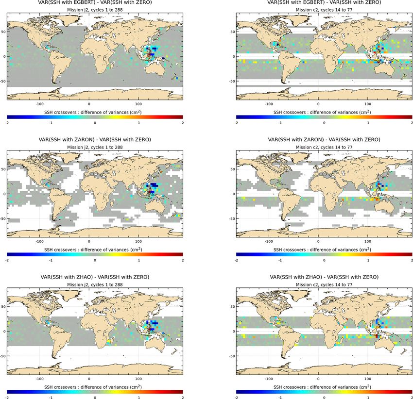
150                                                        L. Carrere et al.: Accuracy assessment of global internal-tide models

Table 1. List of the participating IT models. Most of the models are global models except one that is currently available in only two areas
(Hawaii and Azores, noted in italic). E – empirical model; A – assimilative model; H – hydrodynamic model. Abbreviations used for altimeter
missions: TP – TOPEX/Poseidon; J1 – Jason-1; J2 – Jason-2; EN – Envisat; GFO – GEOSAT Follow-On; C2 – CryoSat-2; AL – AltiKa.

  Model name         Type of   Grid resolution   Constituents tested   Altimeter data used              Authors
                     model           provided
  DUSHAW             E                   0.05◦   M2                    TP + J1                          Dushaw (2015)
  EGBERT             A                   0.03◦   M2 , K1 , O1 , S2     ERS-EN + TP-J1-J2                Egbert and Erofeeva (2014, 2002)
  HYCOM              H                   0.08◦   M2                    No data assimilated              Shriver et al. (2014)
  RAY                E                   0.05◦   M2                    GFO + ERS-EN + TP-J1-J2          Ray and Zaron (2016)
  UBELMANN           E                    0.1◦   M2                    All except C2                    Ubelmann et al. (2020)
  ZARON (HRET)       E                   0.05◦   M2 , K1 , O1 , S2     TP-J1-J2 + ERS-EN-AL + GFO       Zaron (2019)
  ZHAO               E                    0.1◦   M2 , K1 , O1 , S2     GFO + ERS-EN + TP-J1-J2          Zhao et al. (2016)

the mesoscales and coherent M2 internal tides. Indeed, the              Jason missions, the ERS–Envisat–AltiKa missions and the
mesoscale signal is known to introduce errors in the tidal es-          GEOSAT Follow-On mission (Zaron, 2019). Standard atmo-
timation (non-zero harmonics in a finite time window). To               spheric path delay and environmental corrections are applied
mitigate that issue, most existing methods subtract the low-            to the data, including the removal of the barotropic tide us-
frequency altimetry field from AVISO (Archiving, Valida-                ing the GOT4.10c model and the removal of an estimate for
tion and Interpretation of Satellite Oceanographic data) as             the mesoscale sea level anomaly using a purpose-filtered ver-
a proxy for mesoscales (e.g., Ray and Zaron, 2016). How-                sion of the Ssalto/Duacs multi-mission L4 sea level anomaly
ever, the estimate of the mesoscale is itself contaminated              product (Zaron and Ray, 2018). Conventional harmonic anal-
by internal tides (e.g., Zaron and Ray, 2018) aliased into a            ysis is then used to compute harmonic constants at each point
low frequency, which also introduces errors. For these rea-             along the nominal 1 Hz ground tracks (Carrere et al., 2004),
sons, Clément Ubelmann (personnal communication, 2017)                  and these data are used as inputs for subsequent steps.
proposed here a simultaneous estimation, accounting for the                 HRET was initially developed to evaluate plausible spa-
covariances of mesoscales and internal tides in a single in-            tial models for the baroclinic tides, seeking ways to improve
version. In practice, these covariances are expressed as a re-          on some previous models (Zhao et al., 2012; Ray and Zaron,
duced wavelet basis (local in time and space) for mesoscales            2016). It uses a local representation of the wave field as a sum
and as a plane wave basis (local in space only) for internal            of waves modulated by an amplitude envelope consisting of a
tides. The plane wave wavelength and phase speed rely on                second-order polynomial, thus generalizing the spatial signal
the first and second Rossby radii of deformation climatol-              model used in previous plane wave fitting (Ray and Mitchum,
ogy by Chelton et al. (1998). Although the inversion cannot             1997; Zhao et al., 2016). The details of the implementation
be done explicitly (because of the long time window extend-             in HRET differ in additional ways from previous approaches.
ing the basis size for the mesoscale), a variational minimiza-          Specifically, the wavenumber modulus and direction of each
tion allows for a converged solution after about 100 iterations         wave component are determined by local two-dimensional
(typical degree of freedom for the problem). For this study,            Fourier analysis of the along-track data, and the coefficients
only the M2 internal-tide solution (for mode 1 and mode 2) is           in the spatial model are determined by weighted least-squares
considered, but the mesoscale solution is also of interest be-          fitting to along-track slope data – the latter removes the need
cause the internal-tide contamination should be minimized               for rather arbitrary along-track high-pass filtering used in
compared to the standard AVISO processing.                              other estimates. Hence, the model is fully empirical in the
   The method is further described in Ubelmann et al. (2020).           sense that it does not use an a priori wavenumber dispersion
Further improvements are expected after introducing addi-               relation.
tional tide components in the same inversion and after con-                 The above-described approach to building local models
sidering slow (or seasonal) variation in the phases.                    for the baroclinic waves is applied to overlapping patches
                                                                        of the ocean, which are then blended and smoothly interpo-
ZARON                                                                   lated on a uniform latitude–longitude grid. Using the stan-
                                                                        dard error estimates from the original harmonic analysis and
The High Resolution Empirical Tide (HRET) model pro-                    goodness-of-fit information from the spatial models, a mask
vides an empirical estimate for the baroclinic tides at the             is prepared which smoothly damps the model fields to zero
M2 , S2 , K1 and O1 frequencies, as well as the annual mod-             in regions where the estimate is believed to be too noisy to be
ulations of M2 , denoted MA2 and MB2. The development                   useful. These are generally regions near the coastline where
of HRET begins with assembling time series of essentially               the number of data used are reduced or regions in western
all the exact-repeat mission altimetry along the reference              boundary currents or the Southern Ocean where the baro-
and interleaved orbit ground tracks of the TOPEX/Poseidon–

Ocean Sci., 17, 147–180, 2021                                                                 https://doi.org/10.5194/os-17-147-2021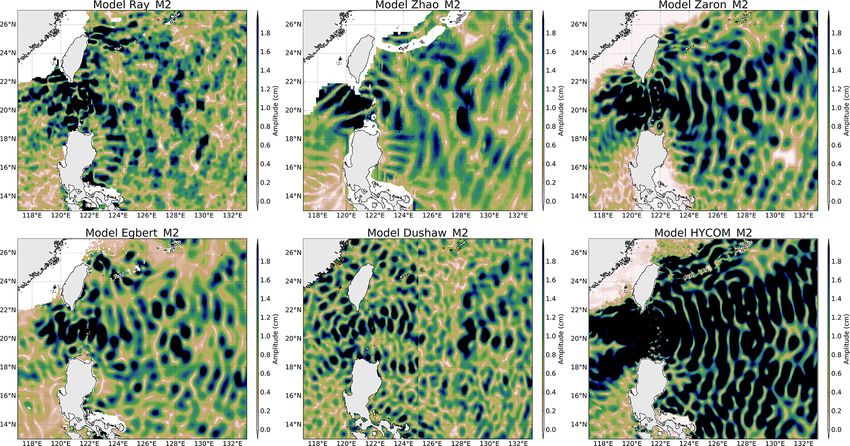
L. Carrere et al.: Accuracy assessment of global internal-tide models                                                            151

clinic tides cannot be distinguished from the continuum of           teraction coefficients, which can be given in terms of the
energetic mesoscale variability. HRET version 7.0 was pro-           vertical-mode eigenvalues following the approach of Grif-
vided for the present validation analysis. Note that the model       fiths and Grimshaw (2007). Modes are decoupled wherever
is still being refined and version 8.1 is available at present: it   bathymetric gradients are zero, and for a flat bottom the
has improved O1 relative to the results shown here and made          system reduces to the usual single-mode RG shallow-water
minor changes to the other constituents.                             equations.
                                                                        Within the RG scheme used, the vertical-mode coupling
ZHAO                                                                 terms are dropped to obtain independent equations for the
                                                                     propagation of each mode with spatially variable reduced
This model is constructed by a two-dimensional plane wave            water depth, which are determined from local bathymetry
fit method (Zhao et al., 2016). In this method, internal tidal       and stratification. These simplified equations are identical to
waves are extracted by fitting plane waves using SSH (sea            the linear shallow-water equations used in the OSU Tidal In-
surface height) measurements in individual fitting windows           version Software (OTIS, https://www.tpxo.net/otis, last ac-
(160 km by 160 km for M2 ). Prerequisite wavenumbers are             cess: 17 December 2020; Egbert and Erofeeva, 2002), thus
calculated using climatological ocean stratification profiles.       allowing the use of the assimilation system to map internal
For each window, the amplitude and phase of one plane                tides by simply modifying depth and fitting along-track har-
wave in each compass direction (angular increment 1◦ ) are           monic constants as a sum over a small number of modes.
determined by the least-squares fit. When the fitted ampli-          With some extensions to OTIS, coupling terms for the first
tudes are plotted as a function of direction in polar coordi-        few modes can be included in the dynamics.
nates, an internal tidal wave appears to be a lobe. The largest         This OTIS-RG assimilation scheme has been applied to
lobe gives the amplitude and direction of one internal tidal         construct global maps of first mode temporally coherent
wave. The signal of the determined wave is predicted and             internal-tide elevations. Available exact repeat mission data,
removed from the initial SSH measurements. This procedure            except GFO, were assimilated (TP-Jason, ERS/Envisat), with
can be repeated to extract an arbitrary number of waves (three       the AVISO weekly gridded SSH product used to reduce
waves here). Four tidal constituents M2 , S2 , O1 and K1 are         mesoscale variations before harmonic analysis. Solutions are
mapped separately using their respective parameters and are          computed in overlapping patches (∼ 20◦ × 30◦ ) and then
used in the present paper (model version Zhao16). This map-          merged (via weighted average on overlaps) into a global so-
ping technique dynamically interpolates internal tidal waves         lution. It may be noted that adjacent solutions almost always
at off-track sites using neighboring on-track measurements,          match quite well even without this explicit tapering.
overcoming the difficulty posed by widely spaced ground
tracks. There are a large number of independent SSH mea-             2.3   Hydrodynamic model
surements in each fitting window, compared to a single time
series of SSH measurements used by pointwise harmonic                The hydrodynamic internal-tide solution is provided by the
analysis. As a result, non-tidal noise caused by tidal aliasing      three-dimensional ocean model HYCOM (HYbrid Coordi-
can be efficiently suppressed. This technique resolves multi-        nate Ocean Model), which embeds tides and internal tides
ple waves of different propagation directions; therefore, the        into an eddying general circulation model (Shriver et al.,
decomposed internal-tide fields may provide more informa-            2014). A free simulation, i.e., without any data assimilation,
tion on generation and propagation.                                  is used for the present study; this run used an augmented
                                                                     state ensemble Kalman filter (ASEnKF) to correct the forc-
2.2   Assimilative model                                             ing and reduce the M2 barotropic tidal error to about 2.6 cm
                                                                     (Ngodock et al., 2016). The value of such a simulation is
Gary D. Egbert and Svetlana Y. Erofeeva have developed               to provide some information about the interaction of inter-
a reduced-gravity (RG) data assimilation scheme for map-             nal tides with mesoscales and other oceanic signals in addi-
ping low-mode coherent internal tides (Egbert and Erofeeva,          tion to the internal-tide signal itself, which means that it can
2014) and applied this to a multi-mission dataset to produce         give access to the non-coherent internal-tide signal too. For
global first mode M2 and K1 solutions. This scheme is based          the present study, a 1-year simulation (simulation no. 102 on
on the Boussinesq linear equations for flow over arbitrary to-       year 2014) has been run and a harmonic analysis of the steric
pography with a free surface and horizontally uniform strati-        1 h SSH allowed the extraction of the M2 internal-tide signal
fication. As in Tailleux and McWilliams (2001) and Griffiths         which remains coherent in this period. The non-assimilative
and Grimshaw (2007), vertical dependence of the flow vari-           quality of the simulation makes it entirely independent from
ables are described using flat-bottom modes (which depend            the altimeter database used for the validation. The spatial res-
on the local depth H (x, y)), yielding a coupled system of           olution of the native grid is 1/24◦ , but data have been inter-
(two-dimensional) partial differential equations (PDEs) for          polated on a 1/12.5◦ grid to provide the tidal atlas for the
the modal coefficients for surface elevation and horizontal          present analysis.
velocity. Equations for each mode are coupled through in-

https://doi.org/10.5194/os-17-147-2021                                                             Ocean Sci., 17, 147–180, 2021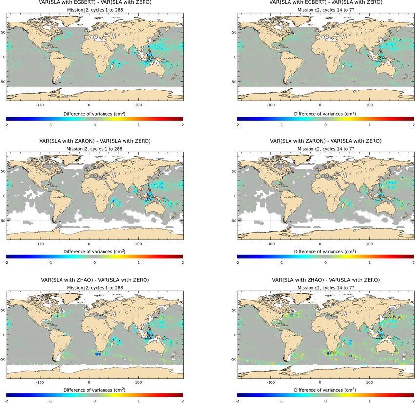
152                                                    L. Carrere et al.: Accuracy assessment of global internal-tide models

3     Comparison of internal-tide models                          be careful as an empirical model might have difficulties sep-
                                                                  arating IT surface signatures from small scales of barotropic
3.1    Qualitative comparison of IT elevations                    tides occurring in these areas. At the strait itself the main
                                                                  wave propagation is expected to be predominantly in the
A first analysis of the model differences consists in visual-     west and/or east directions, which is challenging for empiri-
izing the patterns of IT models’ amplitude in the regions of      cal techniques to recover owing to the primarily north–south
interest defined in Fig. 1. These seven regions are charac-       altimeter track orientations. The problem was discussed in
terized by a well-known and nearly permanent internal-tide        some detail by Ray and Zaron (2016), and their model does
signal, already pointed out by previous studies (Egbert et al.,   indeed have very little eastward-propagating energy from the
2000; Carrere et al., 2004; Nugroho, 2017). From the seven        strait (see also Zhao, 2019a). Plots of the M2 IT for other
regions of interest, the North Pacific area (NPAC) and Luzon      regions defined in Fig. 1 are provided as a Supplement.
regions were selected for the comparison hereafter because            Figure 4 shows the amplitude of the three IT solutions
they are more energetic regions; moreover, all tested models      available for the K1 wave in the Luzon region, where ampli-
are available in the NPAC region and the Luzon area is char-      tudes of the diurnal IT are the most important. Models show
acterized by strong semidiurnal and diurnal baroclinic tides.     large-scale (about 200 km or more) patterns on both sides of
   Figure 2 shows the M2 IT amplitude of each model in            the Luzon Strait. The K1 scales are greater than the M2 scales
the NPAC located around the Hawaiian islands. In this re-         as expected from theoretical wavelengths. The K1 amplitude
gion, all models have similar amplitudes and similar beam         reaches 2 cm on the west side, while patterns and amplitudes
patterns demonstrating northeastward propagation with one         of the models differ on the east side of the strait: ZHAO has
clear northward beam; amplitudes are often greater than           weaker amplitudes and some different spatial patterns, while
2 cm. The amplitude’s pattern varies along IT beams with          ZARON and EGBERT have the solutions that lie closest to
short spatial scales, indicating that most of the models cap-     one to each other. For these three models, the amplitude of
ture a part of the higher-order IT modes: typical 70 km pat-      K1 becomes zero at about 24◦ N when getting close to the
terns are visible corresponding to the second M2 IT mode          K1 critical latitude.
wavelength in this region. The ZHAO solution shows cleaner            Concerning diurnal tides in the global ocean, the ZARON
and smoother patterns likely due to the theoretical plane         solution is not defined over large regions of the world ocean,
wave approximation used for the estimation. RAY, ZHAO             including latitudes poleward of the diurnal-tide critical lati-
and EGBERT propagate until 150◦ W, while ZARON propa-             tude and regions where the IT amplitude is negligible and/or
gates farther to the east and EGBERT has the most attenuated      not separable from background ocean variability. The ZHAO
amplitudes in the region. The UBELMANN and DUSHAW                 solution stops at the diurnal critical latitude, while the EG-
models show similar patterns but both maps are noisier com-       BERT solution is defined over a wider range of latitudes (un-
pared to other solutions. HYCOM also shows similar beams          til 60◦ ).
but with clearly stronger amplitudes, and some noise is also
noticeable in the maps.
   M2 IT amplitudes in the Luzon region are plotted in Fig. 3.    3.2   Quantitative comparison of IT models
Only six models are plotted as UBELMANN is not defined
for this area. The models have an M2 amplitude greater            Following Stammer et al. (2014), the standard deviation (SD)
than 2 cm in the Luzon region, and HYCOM has stronger             of all the IT models listed in Table 1 was computed for
amplitudes than the other models. The IT propagation pat-         each tidal constituent with respect to elevation ηj = ξj e−iσ t ,
tern also shows small spatial scales (of the order of 100 km      where ξj is the time-independent amplitude of a tide compo-
                                                                                                                           √
eastward of the strait) indicating that higher IT modes are       nent at a wet grid point j , σ is tidal frequency and i = −1.
also enhanced at the semidiurnal frequency, but the models        First, the mean elevation of each tidal constituent across
do not agree on a clear common pattern: DUSHAW has a              models taken into account (N) is computed at every grid
rather noisy structure and a discontinuity appears along lon-     point according to
gitude 125◦ E due to the effect of the different computational
patches used to estimate the global solution. All other mod-
els show a strong M2 amplitude across the Luzon Strait; on                1 XN
the east side of the strait, two beams northward and south-       ηmean =           ξ e−iσ t
                                                                                j =1 j
                                                                          N
ward along Taiwan and the Philippines, respectively, are vis-
ible, and a wide eastward beam is visible in the ZARON,                 = Hmean (cos Gmean + i sin Gmean ) e−iσ t ,            (1)
ZHAO and HYCOM maps. The patterns are noisier for the
EGBERT and RAY solutions. The ZARON and HYCOM so-
lutions are close to zero in shallow waters, while RAY, ZHAO      where ξj = Hj cos Gj + i sin Gj with Hj the amplitude
and EGBERT are not defined; DUSHAW is defined in shal-            and Gj the Greenwich phase lag of the tide considered. Then
low waters showing some propagation patterns, but one must        the SD between all involved models (N) can be computed for

Ocean Sci., 17, 147–180, 2021                                                          https://doi.org/10.5194/os-17-147-2021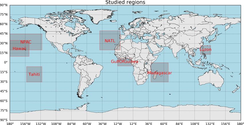
L. Carrere et al.: Accuracy assessment of global internal-tide models 153
Figure 1. Localization of the internal-tide regions studied in the present paper.
each constituent at each grid point according to els. The mean M2 amplitudes reach more than 2 cm in all
1
the known generation sites – in the Pacific, the Indian Ocean
ZT around Madagascar, the Indonesian Seas and in the Atlantic
2
1 XN 1
SDtide = n=1 T
(Re(ηn − ηmean ))2 dt offshore of Amazonia. K1 has a significant mean amplitude
N above 1.5 cm in the Luzon Strait region, in the Philippine Sea
0
and east of Palau and about 0.5–0.7 cm in some regions of the
1 XN 1 h Indian and Pacific oceans.
= n=1 2
Hn cos (Gn )
N The map of M2 SD shows small values, generally below
2 1 cm for M2 , indicating good agreement of the IT models in
− Hmean cos (Gmean )
all IT regions defined in Fig. 1 for the M2 wave; the ratio
i1/2
2 SD / mean amplitude for the M2 wave reaches only 0.2–0.3
+ (Hn sin (Gn ) − Hmean sin (Gmean )) , (2)
around IT generation regions with some clear beam patterns
indicating that models agree with each other in those areas.
where Hn and Gn are the amplitude and the Greenwich phase Some larger SD values are found around Luzon Strait, above
lag of a constituent given by each model, respectively, and Madagascar and in the Indonesian seas. For the diurnal wave
Hmean and Gmean are the mean amplitude and Greenwich K1 , IT models provide coherent information in the Luzon
phase lag computed from all models from Eq. (1). region, in Tahiti and Hawaii and in the Madagascar region.
The computation of the SDtide was performed for the four The mean standard deviation value is computed over the
tidal constituents M2 , S2 , K1 and O1 , after re-gridding bilin- different regions studied. In order to eliminate any residual
early the models to a common 1/20◦ grid. The maps of SD barotropic variability likely existing in the empirical IT mod-
are computed over the global ocean. Note that the DUSHAW els in shallow waters, only data located in the deep ocean are
model was not included in this SD calculation, as it increases used to compute the standard deviation; values are gathered
too much the SD value over the global ocean due to nois- in Table 2. Over all regions, the standard deviation is stronger
ier patterns in wide regions and makes the results difficult to for M2 , consistent with the fact that M2 is the most important
analyze. IT component in the global ocean. The standard deviation is
Global maps shown in Figs. 5 and 6 illustrate the mean largest in the Luzon and Madagascar regions, where models
amplitude and the standard deviation of the M2 and K1 IT give rather different solutions as already seen in the previous
models, respectively. Near-coastal regions, shallow-water re- section.
gions and regions of low signal to noise are masked-out in
the maps as they are not defined in most of the studied mod-
https://doi.org/10.5194/os-17-147-2021 Ocean Sci., 17, 147–180, 2021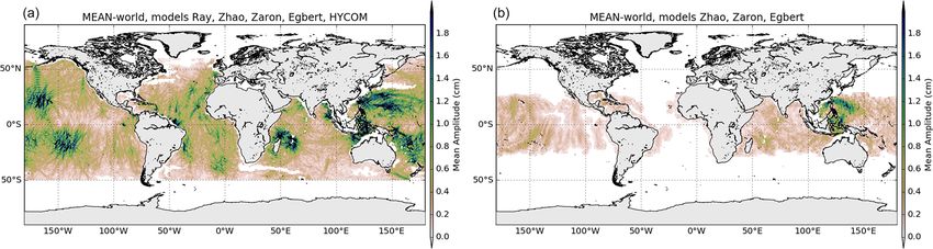
154                                                     L. Carrere et al.: Accuracy assessment of global internal-tide models

Figure 2. Amplitude of the IT models for the M2 tide component in the NPAC region (north Hawaii).

Ocean Sci., 17, 147–180, 2021                                                             https://doi.org/10.5194/os-17-147-2021

L. Carrere et al.: Accuracy assessment of global internal-tide models                                                           155

Figure 3. Amplitude of the IT models for the M2 tide component in the Luzon area.

Figure 4. Amplitude of the IT models for the K1 tide component, in the Luzon area.

  The diurnal K1 tide takes on the largest standard deviation         homogeneous with the DT-2014 standards described in Pujol
value, of 0.25 cm, in the Luzon region, where this diurnal            et al. (2016), except for the tide correction as described be-
component has the most significant amplitudes.                        low.
                                                                         The altimeter period from 1993 onwards is sampled
                                                                      by 12 altimeter missions available on different ground
4     Presentation of the altimeter database and the                  tracks (https://www.aviso.altimetry.fr/en/missions.html, last
      method of comparison                                            access: 17 December 2020). For the purpose of the present
                                                                      study, we use the databases for two different missions:
4.1    The altimeter database

The altimeter measurements used correspond to the level-
2 altimeter product L2P, with 1 Hz along-track res-                      – Jason-2 (denoted J2 in the text and figures) is a refer-
olution (LRM), produced and distributed by Aviso+                          ence mission flying in the reference TP track with a 10 d
(https://www.aviso.altimetry.fr/en/data/, last access: 17 De-              cycle and sampling latitudes between ± 66◦ ; the entire
cember 2020 AVISO), as part of the Ssalto ground process-                  mission time span in the reference track can be used for
ing segment. The version of the products considered is nearly              the study which represents nearly 8 years of data;

https://doi.org/10.5194/os-17-147-2021                                                              Ocean Sci., 17, 147–180, 2021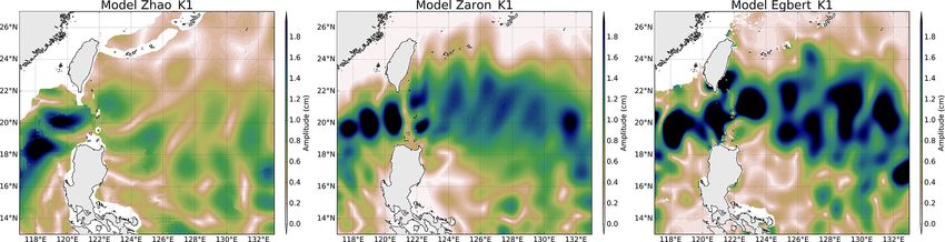
156                                                     L. Carrere et al.: Accuracy assessment of global internal-tide models

Figure 5. Global maps of mean amplitude of the M2 (a) and K1 (b) IT models (cm).

Figure 6. Global maps of standard deviation of the M2 (a) and K1 (b) IT models (cm).

  – CryoSat-2 (denoted C2 hereafter) is characterized by a            Table 2. Spatial-mean SD (cm) of the M2 and K1 IT models for
    drifting polar orbit sampling all polar seas and it has a         each studied region.
    nearly repetitive sub-cycle of about 29 d.
                                                                                Region           SD M2 (cm)    SD K1 (cm)
   The mission’s time series and the number of cycles used
                                                                                Tahiti                  0.36          0.07
for the present study are listed in Table 3. It is worth pointing
                                                                                Hawaii                  0.33          0.07
out that much of the T/P and Jason data have been used in                       Madagascar              0.46          0.10
most of the IT empirical solutions tested (see Table 1), but                    Gulf of Guinea          0.21          0.07
all models are independent of CryoSat-2 mission data.                           Luzon                   0.54          0.25
   Due to sub-optimal time sampling, altimeters alias the                       NATL                    0.15             –
tidal signal to much longer periods than the actual tidal pe-                   NPAC                    0.20             –
riod. The aliased frequencies of the four main tidal waves
studied are listed in Table 3 for the two orbits used. It is no-
ticeable that the diurnal tide K1 is the most difficult to ob-
serve with satellite altimetry as it is aliased to the semiannual        – tide includes the geocentric barotropic tide, the solid
period by the J2 orbit and to a nearly 4-year period by the C2             Earth tide and the pole tide corrections. The geo-
satellite orbits. C2 aliasing periods are very long compared               centric barotropic tide correction was updated com-
to Jason’s ones.                                                           pared to the altimetry standards listed in Pujol et
   The altimeter sea surface height (SSH) is defined as the                al. (2016) and comes from the FES2014b tidal
difference between orbit and range, corrected from several                 model (https://www.aviso.altimetry.fr/en/data/, last ac-
instrumental and geophysical corrections as expressed be-                  cess: 17 December 2020; Carrere et al., 2016a; Lyard et
low:                                                                       al., 2020);

SSH = orbit − range − tide − IT − other_corr,                (3)
                                                                         – IT is the internal-tide correction, taken one by one from
where                                                                      each model studied in this paper;

Ocean Sci., 17, 147–180, 2021                                                             https://doi.org/10.5194/os-17-147-2021
L. Carrere et al.: Accuracy assessment of global internal-tide models 157
Table 3. Description of the altimeter database for the validation Third, the impact of each IT model on SSH can be esti-
study, along with the associated aliasing periods for the main tidal mated for short temporal scales (time lags lower than 10 d),
components. which are the main concern here as we consider the main
high-frequency tidal components M2 , K1 , O1 and S2 . More-
Mission J2 C2
over, these short temporal scales also impact climate studies
Repeat period (d) 9.9156 sub-cycle of 28.941 since high temporal-frequency errors increase the formal es-
Cycles used 1–288 (8 years) 14–77 (5 years)
timation error of long-timescale signals (Ablain et al., 2016;
Time period 12 Jul 2008–6 May 2016 28 Jan 2011–22 Feb 2016
Darwin name Aliasing (d) Aliasing (d) Carrere et al., 2016b). The impact of using each of the studied
O1 45.7 294.4 corrections on the SSH performances is estimated by com-
KL1 173.2 1430 puting the SSH differences between ascending and descend-
M2 62.1 370.7
S2 58.7 245.2
ing tracks at crossovers of each altimeter. Crossover points
with time lags shorter than 10 d within one cycle are selected
in order to minimize the contribution of the ocean variability
at each crossover location. For the purpose here, we avoid all
– other_corr includes the dynamic atmospheric correc-
strong assumptions about internal tide and assume coherent
tion, the wet tropospheric correction, the dry tropo-
internal tides have short autocorrelation scales.
spheric correction, the ionospheric correction, the sea
Fourth, the variance of SSH differences at crossover points
state bias correction and complementary instrumen-
is computed on boxes of 4◦ × 4◦ holding all measurements
tal corrections when needed, as described in Pujol et
within the time span of the mission considered according to
al. (2016).
Diff VarSSH = Var(1SSHITi ) − Var(1SSHITzero ), (4)
The sea level anomaly (SLA) is defined by the differ-
ence between the SSH and a mean profile (MP) for repeti- where 1SSHITzero is the SSH differences at crossovers using
tive orbits or a mean sea surface (MSS) for drifting orbits. a zero IT correction within a 4◦ × 4◦ box for the period con-
Mean profiles computed for TOPEX or the Jason orbit for sidered and 1SSHITi is the SSH differences at crossovers us-
the reference period of 20 years (1993–2012), have been ing one of the IT models listed in Table 1 within the same box
used within the present study for the J2 mission (Pujol et and period. The resulting maps give information on the spa-
al., 2016), and the MSS_CNES_CLS_11 also referenced on tiotemporal variance of the SSH differences within each box.
the same 20 years period was used for the C2 drifting or- As SSH differences are considered, this variance estimation
bit mission (https://www.aviso.altimetry.fr/en/data/products/ is twice the variance difference of SLA. A reduction in this
auxiliary-products/mss.html, last access: 17 December 2020; diagnostic indicates an internal consistency of sea level be-
Schaeffer et al., 2012; Pujol et al., 2016; Appendix A). tween ascending and descending passes within a 10 d win-
dow and thus characterizes a more accurate estimate of SSH
4.2 Method of comparison for high frequencies. However, the spatial resolution of this
diagnostic is limited due to the localization of crossovers and
Satellite altimetry databases can be used to evaluate many
the 4◦ resolution of the grid. Particularly for C2, the mission
geophysical corrections and particularly global barotropic
ground tracks’ pattern induces a non-homogeneous spread of
tidal models as already examined by other authors (Stammer
crossovers over the global ocean, with no crossovers around
et al., 2014; Carrere et al., 2016a, b; Lyard et al., 2006; Car-
latitudes 0◦ and ± 50◦ . For J2, all latitudes are covered with
rere, 2003). We propose using a similar approach to validate
crossovers but the number of points is not homogeneous over
the concurrent IT models listed in Table 1.
the ocean: it is limited at the Equator and increases towards
First, we generate the corresponding IT correction for each
the poles.
along-track altimeter measurement, computed from the inter-
Fifth, along-track SLA statistics can be calculated from
polation of each IT atlas onto the satellites’ ground tracks and
1 Hz altimetric measurements and allow for a higher spatial
the use of a tidal prediction algorithm. Each tidal component
resolution in the analysis. The maps of the variance differ-
is considered separately for the clarity of the analysis, keep-
ence of SLA using either the IT correction tested or the ref-
ing in mind that the various IT models do not all contain the
erence ZERO correction are computed on boxes of 2◦ × 2◦
same waves.
according to
Second, the altimeter SSH using IT corrections from each
model tested can then be computed, and the differences in the Diff VarSLA = Var(SLAITi ) − Var(SLAITzero ), (5)
sea level contents are analyzed for different time and spatial
scales. In particular, considering several altimeters allows the where SLAITi (or SLAITzero ) are the SLA computed using
study of different temporal periods. As the missions consid- one of the IT corrections listed in Table 1 (or using the
ered, J2 and C2, have different ground tracks and different zero IT correction) in the period considered and within one
orbit (cycle) characteristics, several aliasing characteristics 2◦ × 2◦ box. Although high-frequency signals are aliased in
are tested. the lower-frequency band following the application of the
https://doi.org/10.5194/os-17-147-2021 Ocean Sci., 17, 147–180, 2021158 L. Carrere et al.: Accuracy assessment of global internal-tide models
Nyquist theory to each altimeter sampling, SLA time se- the EGBERT, ZARON, ZHAO and RAY models have simi-
ries contain the entire ocean variability spectrum. The SLA lar mean performances, but RAY reduces a bit more the J2
variance reduction diagnostic shows an improvement of the variance globally (0.34 cm2 ).
studied IT correction, on the condition that the correction is Figure 8 displays the maps of along-track J2 SLA vari-
decorrelated from the sea level. ance differences using the M2 IT correction from each model
Sixth, the mean of these variance reduction estimations and a ZERO reference correction. Spatial patterns are simi-
at crossovers and for along-track SLA is computed for each lar to those in Fig. 7. However, using the along-track SLA
studied region, which allows an easier analysis and compari- allows for a better spatial resolution in the output vari-
son of the performances of the IT model tested. ance maps. In addition, regions of strong IT and regions
Finally, in order to quantify the impact of each IT model of strong ocean currents are more clearly identified. The
on the SLA variance reduction in terms of spatial scales, a DUSHAW model raises SLA variance in several mesoscale
spectral analysis of J2 SLA is performed in the different re- regions (Gulf Stream, Agulhas current, Argentine basin and
gions of interest, and details are given in Sect. 6. Kuroshio currents), likely indicating that the model does
not properly separate IT and other oceanic signals in these
strong-current areas; the ZHAO model also raises the vari-
5 Variance reduction analysis using satellite altimeter ance in those regions slightly, while EGBERT reduces the
data SLA variance in the Gulf Stream and Agulhas regions. HY-
COM raises the variance over wider regions in the three
This section gathers the validation results of each IT model oceans than the empirical and assimilative models do: this
using the satellite altimetry databases described previously. is likely due to its intrinsic characteristic of the free hydro-
For the clarity of the analysis, each IT correction is compared dynamic model which may induce more phase errors com-
to a reference correction using a ZERO correction. For the pared to constrained or empirical models and also due to the
ZERO correction, no IT correction is applied, as in the actual short HYCOM time series duration used to extract the IT
altimeter geophysical data records version-D and version-E atlas, which induces stronger IT amplitudes (see Ansong et
(GDR-D and GDR-E) processing (Pujol et al., 2016; Taburet al., 2015; Buijsman et al., 2020). These maps also indicate
et al., 2019). The complete diagnostics and analysis are pre- that the four models RAY, EGBERT, ZARON and ZHAO,
sented hereafter for the largest semidiurnal (M2 ) and diurnal reduce the SLA variance in some additional IT areas which
(K1 ) components; results for the second-largest semidiurnal are not specifically investigated in the present study: the In-
(S2 ) and diurnal (O1 ) IT are gathered in the Appendix of the donesia seas and south of Java, north of Sumatra, between
paper. the Solomon Islands and New Zealand in Pacific, off the
Amazonian shelf, and in many regions of the Atlantic Ocean.
5.1 M2 component Mean values, averaged over the strong IT regions identified
in Fig. 1, are given in Table 4: mean J2 SLA variance re-
To investigate and quantify the regional impact of the M2 ductions are weaker than the crossover difference variances
IT corrections, the maps of SSH variance difference at by construction, but they indicate similar conclusions as for
crossovers using either IT correction from each model or a J2 crossover differences: the ZARON model is the most effi-
ZERO reference correction, are plotted for the J2 mission in cient to reduce the SLA variance in all IT regions, except in
Fig. 7. Note that the quantification and the regional analy- NPAC and NATL, where the UBELMANN model is slightly
sis of the M2 IT correction can be performed for the seven more efficient. Mean values over the global ocean are close
IT models participating in the present study. Most of the IT for the four models EGBERT, ZHAO, ZARON and RAY,
models reduce the altimeter SSH variance in all IT regions. with the two last ones showing a slightly better performance
The RAY and ZARON models are the most efficient, with a than others.
variance reduction reaching more than 5 cm2 in many areas. One should note that those J2 results might be biased in
The HYCOM and DUSHAW models reduce SSH variance favor of the empirical models, as J2 data are used in all of
in some locations but also raise the variance locally: mostly them except for the DUSHAW model (see Table 1). To check
in large deep ocean regions where IT signal can be weak in these results, similar diagnostics are computed using the C2
other models for HYCOM, while the DUSHAW model raises altimeter database, as described in Sect. 4.1, which is an inde-
variance mostly in areas of strong currents. Mean values, av- pendent database for all models. Validation results are given
eraged over the strong IT regions shown in Fig. 1, are listed in Figs. 9 and 10 for C2 SSH crossover differences and C2
in Table 4: the more energetic areas for the M2 IT seem to SLA, respectively.
be the Luzon Strait and Hawaii regions with a mean SSH Validations with the C2 database show similar results as
variance reduction greater than 2 cm2 for the ZARON model. for J2, with a significant variance reduction in the C2 SSH
The ZARON model is the most efficient in all areas except differences and SLA for most models in all IT regions; vari-
in the North Atlantic (NATL) region where the UBELMANN ance gain patterns are generally similar but more widely
model reduces slightly more variance. Over the global ocean, spread and stronger in C2 SSH maps compared to J2 par-
Ocean Sci., 17, 147–180, 2021 https://doi.org/10.5194/os-17-147-2021L. Carrere et al.: Accuracy assessment of global internal-tide models 159 Figure 7. Maps of SSH variance differences at crossovers using either the M2 IT correction from each model or a ZERO reference correction in the SSH calculation for the J2 mission (cm2 ). J2 cycles 1–288 have been used. https://doi.org/10.5194/os-17-147-2021 Ocean Sci., 17, 147–180, 2021
160                                                     L. Carrere et al.: Accuracy assessment of global internal-tide models

Figure 8. Maps of SLA variance differences using either the M2 IT correction from each model or a ZERO reference correction in the SLA
calculation for the J2 mission (cm2 ). J2 cycles 1–288 have been used.

Ocean Sci., 17, 147–180, 2021                                                             https://doi.org/10.5194/os-17-147-2021
L. Carrere et al.: Accuracy assessment of global internal-tide models                                                        161

ticularly in the Atlantic Ocean and in the west Pacific. The      the J2 SLA variance mostly in the Luzon Strait or west Pa-
pattern is different for the UBELMANN model in the NATL           cific region and the northern Indonesian seas, where the am-
region, likely due to some inclusion of J2 errors or signal or    plitude of the K1 IT is the most important; a weak variance
larger-scale signals in the model (see Sect. 6). The ground       gain is also visible in the IT regions around Tahiti, Hawaii
track pattern of the C2 orbit explains the lack of crossover      and north of Madagascar but also in some large ocean cur-
data at 0◦ and ± 50◦ latitudes bands. C2 SLA variance maps        rent regions, in the central Indian Ocean and east of Aus-
have similar patterns compared to J2, and some additional IT      tralia. The other maps indicate that ZHAO is less efficient
regions are pointed out, which corroborates the quality of the    than the two others in the Luzon region, while ZARON re-
different IT models tested. Over both C2 SSH and SLA, the         duces slightly more variance for the C2 mission in the west
HYCOM and DUSHAW models show a significant addition               Pacific area.
of variance in some regions, similarly as for J2 results.            The mean statistics of altimeter variance reduction, over
   Mean values for C2 data, averaged over the strong IT re-       the regions defined in Fig. 1, are given in Table 5 for the
gions, are also given in Table 4. Mean C2 SLA variance gains      SLA and the SSH differences of J2 and C2 missions and
are comparable to J2 mission on all IT regions. C2 valida-        for the different regions studied; note that we focus on Lu-
tion results for the M2 IT component show that the ZARON          zon, Tahiti, Hawaii, Madagascar and global areas because
model performs better than other models in most IT regions        mean K1 statistics are not significant in the other regions of
studied, with a maximum reduction in SSH difference vari-         large semidiurnal tides defined in Fig. 1. The values in Ta-
ance of 3.2 cm2 in Luzon and 2.2 cm2 in the Madagascar            ble 5 indicate a significant variance reduction mainly in the
area. RAY reduces variance a bit more in the Tahiti region; on    Luzon region as expected from the analysis of global maps.
average over the global ocean, the ZARON and RAY models           The ZARON and EGBERT models are the most efficient IT
are the most efficient.                                           solutions in the Luzon region, with similar variance gains
                                                                  for both models at C2 crossovers. ZARON shows a signifi-
5.2   K1 component                                                cant variance gain compared to the ZERO correction for both
                                                                  missions tested, reaching 3 and 2.4 cm2 , respectively, for J2
The maps of K1 SSH variance difference at crossovers us-          crossovers and C2 crossovers.
ing the K1 IT correction from EGBERT, ZARON and ZHAO
models are plotted in Fig. 11 for the J2 and C2 missions.
Note that unlike the M2 wave analysis, the quantification         6   Wavelength analysis for the M2 wave
and the regional analysis of the K1 IT correction can be per-
formed for only three IT models participating in the present      In order to quantify the impact of each IT model on the
study that provide a K1 solution, as the diurnal tides are        altimeter SLA variance reduction as a function of spatial
more difficult to detect and sort out by altimetry. The K1        scales, a spectral analysis of J2 along-track SLA is per-
IT solutions are compared to a ZERO reference correction.         formed. This analysis is not conducted for other missions
The three models have different approaches to take into ac-       because the duration of the C2 mission time series used is
count the diurnal tides’ critical latitude and regions where      too short to allow a proper spectral estimation at the aliasing
amplitude of K1 IT is negligible and/or not separable from        frequency of M2 (cycle duration is 370 d for C2). Moreover,
background ocean variability (cf Sects. 2 and 3.1), which ex-     this diagnostic only focuses on the main M2 IT because the
plains the large non-defined regions in ZARON and ZHAO            K1 aliasing frequency by J2 sampling is 173 d (see Table 2),
maps compared to EGBERT. Results show that the three IT           which makes it barely separable from the semiannual ocean
models all reduce the J2 SSH variance strongly in the west        signal.
Pacific or Luzon and Indonesian regions (more than 2 cm2 ),          The J2 SLA spectral analysis is performed for each of the
while a weaker variance reduction is visible in the central In-   IT regions described in Fig. 1. For each area, a frequency–
dian and central Pacific areas (0.5–1 cm2 ). The reduction is     wavenumber spectrum is computed for the along-track SLA
also important for C2 SSH in the east Pacific or Luzon area       and for the SLA corrected from each IT solution; the spectral
and south of Java, and results are noisier in the other oceans    density at a 62 d frequency, which is the aliasing frequency
where diurnal IT is weak, but C2 data are likely less efficient   band of the M2 tidal component by Jason’s orbit, is extracted
for testing the K1 tide due its very long alias compared to M2    in both cases and then the normalized difference of the spec-
tide (see Table 3). The ZARON model reduces slightly more         tral density is computed and plotted as a function of wave-
C2 variance in the southern part of the Indian Ocean.             length. This computation gives an estimation of the percent-
   The maps of SLA variance differences using the EGBERT,         age of energy removed at the M2 frequency thanks to each
ZARON and ZHAO K1 IT models are plotted in Fig. 12 for            IT model correction, as a function of wavelength and for the
the J2 and C2 missions. Spatial SLA patterns are consistent       different regions studied.
with the SSH maps of Fig. 11 and allow a better spatial res-         Results for the different regions are gathered in Fig. 13
olution compared to SSH maps as also noted for M2 results:        and show that all empirical models generally manage to re-
using the EGBERT model allows a significant reduction in          move an important amount of coherent IT energy for the first

https://doi.org/10.5194/os-17-147-2021                                                          Ocean Sci., 17, 147–180, 2021
You can also read