Adversarial examples for Deep Learning Cyber Security Analytics
←
→
Page content transcription
If your browser does not render page correctly, please read the page content below
Adversarial examples for Deep Learning Cyber Security Analytics

                                                                     Alesia Chernikova                                      Alina Oprea
                                                                   Northeastern University                            Northeastern University

                                         Abstract—We consider evasion attacks (adversarial exam-            PDF malware detection [62], [67] and malware classifica-
                                         ples) against Deep Learning models designed for cyber se-          tion [31], [63], but these applications use binary features.
                                         curity applications. Adversarial examples are small modifica-      Recently, Kulynych et al. [41] introduce a graphical frame-
                                         tions of legitimate data points, resulting in mis-classification   work for general evasion attacks in discrete domains, that
                                         at testing time. We propose a general framework for crafting       constructs a graph of all possible transformations of an
                                         evasion attacks that takes into consideration the dependen-        input and selects a set of minimum cost to generate an
                                         cies between intermediate features in model input vector, as       adversarial example. The previous work, however, cannot
arXiv:1909.10480v2 [cs.CR] 31 Jan 2020

                                         well as physical-world constraints imposed by the applica-         yet handle evasion attacks in security applications that
                                         tions. We apply our methods on two security applications,          respect complex feature dependencies, as well as physical-
                                         a malicious connection and a malicious domain classifier, to       world constraints.
                                         generate feasible adversarial examples in these domains. We             In this paper we introduce a novel framework for
                                         show that with minimal effort (e.g., generating 12 network         crafting adversarial attacks in cyber security domain that
                                         connections), an attacker can change the prediction of a           respects the mathematical dependencies given by common
                                         model from Malicious to Benign. We extensively evaluate            operations applied in feature space and enforces at the
                                         the success of our attacks, and how they depend on several         same time the physical-world constraints of specific appli-
                                         optimization objectives and imbalance ratios in the training       cations. At the core of our framework is an iterative opti-
                                         data.
                                                                                                            mization method that determines the feature of maximum
                                                                                                            gradient of attacker’s objective at each iteration, identifies
                                                                                                            the family of features dependent on that feature, and
                                         1. Introduction                                                    modifies consistently all the features in the family, while
                                                                                                            preserving an upper bound on the maximum distance and
                                             Deep learning has reached super-human performance              respecting the physical-world application constraints.
                                         in machine learning (ML) tasks for classification in diverse            Our general framework needs minimum amount of
                                         domains, including image classification, speech recogni-           adaptation for new applications. To demonstrate this, we
                                         tion, and natural language processing. Still, deep neural          apply our framework to two distinct applications. The first
                                         networks (DNNs) are not robust in face of adversarial              is a malicious network traffic classifier for botnet detection
                                         attacks, and their vulnerability has been demonstrated ex-         (using a public dataset [27]), in which an attacker can
                                         tensively in many applications, with the majority of work          insert network connections on ports of his choice that re-
                                         in adversarial ML being performed in image classification          spect the physical network constraints (e.g., TCP and UDP
                                         tasks (e.g, [65], [10], [29], [42], [54], [14], [48], [5]).        packet sizes) and a number of mathematical dependencies.
                                             ML started to be used more extensively in cyber                The second application is malicious domain classification
                                         security applications in academia and industry, with the           using features extracted from web proxy logs (collected
                                         emergence of a a new field called security analytics.              from a large enterprise) that involves a number of sta-
                                         Among the most popular applications of ML in cyber                 tistical and mathematical dependencies in feature space.
                                         security we highlight malware classification [6], [9], [56],       We demonstrate that the attacks are successful in both
                                         malicious domain detection [47], [12], [3], [7], [51], and         applications, with minimum amount of perturbation. For
                                         botnet detection [32], [66]. In most of these applications,        instance, by inserting 12 network connections an attacker
                                         the raw security datasets (network traffic or host logs)           can change the classification prediction from Malicious to
                                         are not used directly as input to the DNN, but instead an          Benign in the first application. We perform detailed evalu-
                                         intermediate feature extraction layer is defined by domain         ation to test: (1) if our attacks perform better than several
                                         experts to generate inputs for neural networks (or other           baselines; (2) if the selection of the optimization objective
                                         ML models). There are efforts to automate the feature              impacts the attack success rate; (3) how the imbalance
                                         engineering aspect (e.g., [38], but it is not yet a common         ratio between the Malicious and Benign classes in training
                                         practice. One of the challenges of adapting ML to work             changes the success of the attack; (4) if features modified
                                         in these domains is the large class imbalance during               by the attack are the features with highest importance.
                                         training [7]. Therefore, adversarial attacks designed on           We also test several approaches for performing the attack
                                         continuous domains (for instance, in image classification)         under a weaker threat model, through transferability from
                                         need to be adapted to take into account the specifics of           a substitute model to the original one, or by adapting
                                         cyber security applications.                                       existing black-box attacks. Finally, we test the resilience
                                             Initial efforts to design adversarial attacks at testing       of adversarial training as a defensive mechanism in this
                                         time (called evasion attacks) for discrete domains are             setting.
                                         underway in the research community. Examples include                    To summarize, our contributions are:
1)    We introduce a general evasion attack framework       attack model, in which the attacker has information about
         for cyber security that respects mathematical fea-    the feature representation of the underlying classifier, but
         ture dependencies and physical-world constraints.     not exact details on the ML algorithm and training data.
   2)    We apply our framework with minimal adapta-               In the considered applications, training data comes
         tion to two distinct applications using different     from security logs ollected at the border of an enterprise
         datasets and feature representations: a malicious     or campus network. We assume that the attacker compro-
         network connection classifier, and a malicious        mises at least one machine on the internal network, from
         domain detector, to generate feasible adversarial     where the attack is launched. The goal of the attacker is
         examples in these domains.                            to modify its network connections to evade the classifier’s
   3)    We extensively evaluate our proposed framework        Malicious prediction in a stealthy manner (i.e., with mini-
         for these applications and quantify the amount        mum perturbation). We assume that the attacker does not
         of effort required by the attacker to bypass the      have access to the security monitor that collects the logs.
         classifiers, for different optimization objectives    That would result in a much more powerful attack, which
         and training data imbalance ratios.                   can be prevented with existing techniques (e.g., [13]).
   4)    We evaluate the transferability of the proposed
         evasion attacks between different ML models           2.3. Evasion Attacks against Deep Neural Net-
         and architectures and test the effectiveness of       works
         performing black-box attacks.
   5)    We measure the resilience of adversarially-               We describe several evasion attacks against DNNs:
         trained models against our attacks.                   projected gradient descent-based attacks and the penalty-
Organization. We provide background material in Sec-           based attack of Carlini and Wagner.
tion 2. We discuss the challenges for designing evasion        Projected gradient attacks. This is a class of attacks
attacks in cyber security and introduce our general frame-     based on gradient descent for objective minimization, that
work in Section 3. We instantiate our framework for the        project the adversarial points to the feasible domain at
two applications of interest in Section 4. We extensively      each iteration. For instance, Biggio et al. [10] use an
evaluate our framework in Sections 5 and 6, respectively.      objective that maximizes the confidence of adversarial
Finally, we discuss related work in Section 7 and conclude     examples, within a ball of fixed radius in L1 norm. Madry
in Section 8.                                                  et al. [48] use the loss function directly as the optimization
                                                               objective and use the L2 and L∞ distances for projection.
2. Background                                                  C&W attack. Carlini and Wagner [14] solve the follow-
                                                               ing optimization problem to create adversarial example
2.1. Deep Neural Networks for Classification                   against CNNs used for multi-class prediction:
                                                                          δ = arg min ||δ||2 + c · h(x + δ)
    A feed-forward neural network (FFNN) for binary            h(x + δ) = max(0, max(Zk (x + δ) : k 6= t) − Zt (x + δ)),
classification is a function y = F (x) from input x ∈ Rd                where Z() are the logits of the DNN.
(of dimension d) to output y ∈ {0, 1}. The parameter
vector of the function is learned during the training phase         This is called the penalty method, and the optimization
using back propagation over the network layers. Each           objective has two terms: the norm of the perturbation
layer includes a matrix multiplication and non-linear acti-    δ , and a function h(x + δ) that is minimized when the
vation (e.g., ReLU). The last layer’s activation is sigmoid    adversarial example x + δ is classified as the target class
σ for binary classification: y = F (x) = σ(Z(x)), where        t. The attack works for L0 , L2 , and L∞ norms.
Z(x) are the logits, i.e., the output of the the penultimate
layer. We denote by C(x) the predicted class for x. For        3. Methodology
multi-class classification, the last layer uses a softmax
activation function.                                               In this section, we start by describing the classification
                                                               setting in cyber security analytics. Then we devote the
2.2. Threat Model                                              majority of the section to describe evasion attacks for
                                                               cyber security, mention challenges of designing them, and
    Adversarial attacks against ML algorithms can be           present our new attack framework that takes into consid-
developed in the training or testing phase. In this work, we   eration the specific constraints of security applications.
consider testing-time attacks, called evasion attacks. The
DNN model is trained correctly and the attacker’s goal         3.1. ML classification in cyber security
is to create adversarial examples at testing time. In secu-
rity settings, typically the attacker starts with Malicious         In standard computer vision tasks such as image clas-
points that he aims to minimally modify into adversarial       sification, the raw data (image pixels) is used directly as
examples classified as Benign.                                 input into the neural network models. In contrast, in cyber
    We consider initially for our optimization framework       security, domain expertise is still required to generate
a white-box attack model, in which the attacker has full       intermediate features from the raw data (e.g., network
knowledge of the ML system. White-box attacks have             traffic or endpoint data) (see Figure 1).
been considered extensively in previous work, e.g., [29],           ML is commonly used in cyber security for classifi-
[10], [14], [48] to evaluate the robustness of existing ML     cation of Malicious and Benign activity (e.g., [47], [12],
classification algorithms. We also consider a more realistic   [51]). A raw dataset R is initially collected (for example,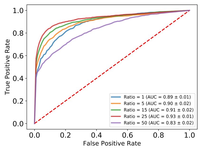
Figure 1: Neural network training for image classification (left) and for cyber security analytics (right).

pcap files or Netflow logs), and feature extraction is                Several previous work address evasion attacks in dis-
performed by applying different operators, such as Max,           crete domains. The evasion attack for malware detection
Min, Avg, and Total. The training dataset Dtr has N train-        by Grosse et al. [30], which directly leverages JSMA [54],
ing examples: Dtr = {(x(1) , L(1) ), . . . , (x(N ) , L(N ) )},   modifies binary features corresponding to system calls.
each example x(i) being a d-dimensional feature vector:           Kolosnjaji et al. [39] use the attack of Biggio et al. [10]
          (i)          (i)
x(i) = (x1 , . . . , xd ). Features of the training dataset are   to append selected bytes at the end of the malware file.
most of the time obtained by application of operator Opj          Suciu et al. [63] also append bytes in selected regions of
                      (i)
on the raw data xj = Opk (R). The set of all supported            malicious files. Kulynych et al. [41] introduce a graphical
operators or functions applied to the raw data is denoted         framework in which an adversary constructs all feasible
by O. A data point x = (x1 , . . . , xd ) in feature space is     transformation of an input, and then uses graph search
feasible if there exists some raw data r such as for all j ,      to determine the path of minimum cost to generate an
there exists a operator Opk ∈ O with xj = Opk (r). The            adversarial example.
set of all feasible points for raw data R and operators               Neither of these approaches are applicable to our gen-
O are called Feasible Set(R, O). An example of feasible           eral setting. First, in the considered applications features
and unfeasible points is illustrated in Table 1.                  have numerical values and the evasion attacks developed
                                                                  for malware binary features [30], [39], [63] are not ap-
                Feature     Feasible   Infeasible                 plicable. Second, none of these attacks guarantees the
              Frac empty       0.2         0.5                    feasibility of the resulting adversarial vector in terms of
               Frac html      0.13        0.13                    mathematical relationships between features. We believe
              Frac image      0.33        0.33
              Frac other      0.34         0.4
                                                                  that crafting adversarial examples that are feasible, and
                                                                  respect all the application constraints and dependencies to
TABLE 1: Example of feasible and infeasible features.             be a significant challenge. Once application constraints are
The features denote the fraction of URLs under a domain           specified, the resulting optimization problem for creating
that have certain content type (e.g., empty, html, image,         adversarial examples includes a number of non-linear
and other). The sum of all the features is 1 in the feasible      constraints and cannot be solved directly using out-of-
example, but exceeds 1 in the unfeasible one.                     the-box optimization methods.

    As in standard supervised learning, the training exam-        3.3. Overview of our approach
ples are labeled with a class L(i) , which is either Malicious
or Benign. Malicious examples are obtained by different
                                                                      To address these issues, we introduce a framework
methods, including using blacklists, honeypots, or running
                                                                  for evasion attacks that preserves a range of feature de-
malware in a sandbox. A supervised ML model (classifier)
                                                                  pendencies and guarantees that the produced adversarial
f is selected by the learning algorithm from a space of
                                                                  examples are within the feasible region of the domain.
possible hypothesis H to minimize a certain loss function
                                                                  Our framework supports two main types of constraints:
on the training set.
                                                                  Mathematical feature dependencies: These are dependen-
                                                                  cies created in the feature extraction layer. For instance,
3.2. Limitations and challenges                                   by applying several mathematical operators (Max, Min,
                                                                  Total) over a set of raw log data, we introduce feature
    Existing evasion attacks are mostly designed and              dependencies. See the example in Figure 3 for Bro (or
tested for image classification, where adversarial examples       Zeek) connection log events and several dependent fea-
have pixel values in a fixed range (e.g., [0,1]) and can be       tures constructed using these operators. For instance, a
modified independently in continuous domains [14], [48],          Bro connection includes the number of packets sent and
[5]. However, most security datasets are discrete, resulting      received, and we define the Min, Max, and Total number
in feature dependencies and physical-world constraints to         of packets sent and received by the same source IP on
ensure certain application functionality.                         a particular port (within a fixed time window). We use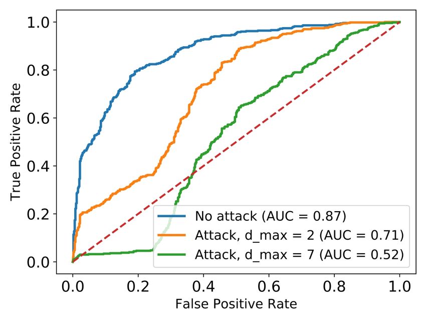
the terminology family of features to denote a subset of          function UPDATE DEP (line 32). We need to define the
features that are inter-connected and need to be updated          function UPDATE DEP for each application, but we use a
simultaneously. For the Bro example, the features defined         set of building blocks that are reusable. Once all features
for each port (e.g., 80, 53, 22) are dependent as they are        in the family have been updated, there is a possibility
generated from all the connections on that port.                  that the update data point exceeds the allowed distance
Physical-world constraints: These are constraints imposed         threshold from the original point. If that is the case, the
by the real-world application. For instance, in the case of       algorithm backtracks and performs a binary search for the
network traffic, a TCP packet has maximum size 1500               amount of perturbation added to the representative feature
bytes.                                                            (until it finds a value for which the modified data point is
    Our starting point for the attack framework are               inside the allowed region).
gradient-based optimization algorithms, including pro-            2. If the feature of maximum gradient does not belong to
jected [10], [48] and penalty-based [14]. Of course, we           any feature family, then it can be updated independently
cannot apply these attacks directly since they will not           from other features. The feature is updated using the
preserve the feature dependencies. To overcome this, we           standard gradient update rule (line 13). This is followed
use the values of the objective gradient at each iteration        by a projection Π2 within the feasible ball in L2 norm.
to select features of maximum gradient values. We create              We currently support two optimization objectives:
feature-update algorithms for each family of dependencies         Objective for Projected attack. We set the objective
that use a combination of gradient-based method and               G(x) = Z1 (x), where Z1 is the logit for the Malicious
mathematical constraints to always maintain a feasible            class, and Z0 = 1 − Z1 for the Benign class:
point that satisfies the constraints. We also use various
                                                                                    δ = arg min Z1 (x + δ),
projection operators to project the updated adversarial
                                                                                       s.t. ||δ||2 ≤ dmax ,
examples to feasible regions of the feature space.
                                                                                  x + δ ∈ Feasible Set(R, O)

3.4. Proposed Evasion Attack Framework                            We need to ensure that the adversarial example is in the
                                                                  feasible set to respect the imposed constraints.
    We introduce here our general evasion attack frame-           Objective for Penalty attack. The penalty objective for
work for creating adversarial examples at testing time for        binary classification is equivalent to:
binary classifiers. In the context of security applications,             δ = arg min ||δ||2 + c · max(0, Z1 (x + δ)),
the main goal of the attacker is to ensure that a Malicious                     x + δ ∈ Feasible Set(R, O)
data point is classified as Benign after applying a min-
imum amount of perturbation to it. We consider binary             Our general evasion attack framework can be used for
classifiers designed using FFNN architectures. For mea-           different classifiers, with different features and constraints.
suring the amount of perturbation added by the original           The components that need to be defined for each applica-
example, we use the L2 norm.                                      tion are: (1) the optimization objective G for computing
    Algorithm 1 and Figure 2 describes the general frame-         adversarial examples; (2) the families of dependent fea-
work. The input consists of: an input sample x with label y       tures and family representatives; (3) the UPDATE DEP
(typically Malicious in security applications); a target label    function that performs feature updates per family; (4) the
t (typically Benign); the model prediction function C ; the       projection operation to respect the constraints.
optimization objective G; maximum allowed perturbation
dmax ; the subset of features FS that can be modified; the        4. Evasion Attacks for Concrete Security Ap-
features that have dependencies FD ⊂ FS ; the maximum             plications
number of iterations M and a learning rate α for gradient
descent. The set of features with dependencies are split              We describe in this section our framework instantiated
into families of features. A family is defined as a subset of     to two cyber security applications, a malicious network
FD such that features within the family need to be updated        connection classifier, and a malicious domain classifier.
simultaneously, whereas features outside the family can be        We emphasize that our framework is applicable to other
updated independently.                                            security applications, such as malware classification, web-
    The algorithm proceeds iteratively. The goal is to            site fingerprinting, and malicious communication detec-
update the data point in the direction of the gradient (to        tion. For each of these, the application-specific constraints
minimize the optimization objective), while preserving            need to be encoded and respected when feature updates
the family dependencies, as well as the physical-world            are performed.
constraints. In each iteration, the gradients of all modifi-
able features are computed, and the feature of maximum            4.1. Malicious Connection Classifier
gradient is selected. The update of the data point x in the
direction of the gradient is performed as follows:                    Network traffic includes important information about
1. If the feature of maximum gradient belongs to                  communication patterns between source and destination
a family with other dependent features, function                  IP addresses. Classification methods have been applied
UPDATE FAMILY is called (line 10). Inside the function,           to labeled network connections to determine malicious
the representative feature for the family is computed (this       infections, such as those generated by botnets [12], [7],
needs to be defined for each application). The representa-        [35], [51]. Network data comes in a variety of formats,
tive feature is updated first, according to its gradient value,   but the most common include net flows, Bro logs, and
followed by updates to other dependent features using             packet captures.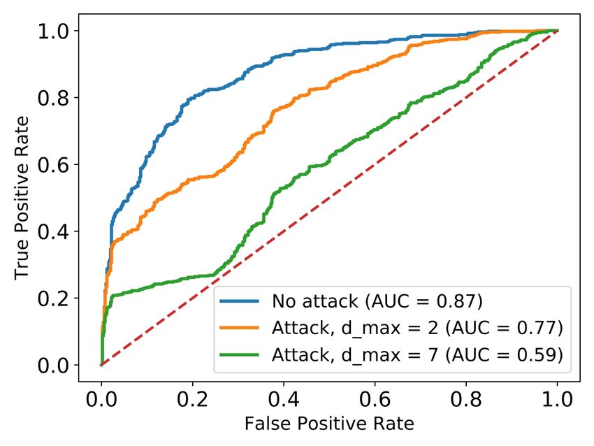
Figure 2: Evasion Attack Framework

                              Time        Src IP            Dst IP        Prot.     Port     Sent      Recv.       Sent    Recv. Duration
                                                                                             bytes     bytes      packets packets
                              9:00:00   147.32.84.59     77.75.72.57        TCP       80      1065      5817            10           11      5.37

                   Raw Bro    9:00:03   147.32.84.59     81.27.192.20      UDP        53       48        48             1             1     0.0012
                   log data   9:00:05   147.32.84.59    87.240.134.159      TCP       80       950       340            7             5     25.25
                              9:00:12   147.32.84.59      77.75.77.9        TCP       80      1256       422            5             5     0.0048

                                                             Port 22         Port 80         Port 53         Port 443

                          Family of features              Packet                    Bytes            Duration                 Traffic
                             for port 80                 features                 features           features                statistics

                                                                                                                  Operator

                                                Min    Max     Sum                                              Min      Max         Sum
                              Sent Packets      5      10      22        Representative         Sent Bytes      950      1256        3271
                                                                            feature
                              Recv. Packets     5      11      21                               Recv. Bytes     340      5817        6579

            Figure 3: Example of Bro logs and feature family per port for malicious connection classifier.

Problem definition: dataset and features. We leverage                                      applications, including: HTTP (80), SSH (22), and DNS
a public dataset of botnet traffic that was captured in at                                 (53). We also add a category called OTHER for connec-
the CTU University in the Czech Republic, called CTU-                                      tions on other ports. We aggregate the communication on
13 dataset [27]. The dataset include Bro connection logs                                   a port based on a fixed time window (the length of which
with communications between internal IP addresses (on                                      is a hyper-parameter). For each port, we compute traffic
the campus network) and external ones. The dataset has                                     statistics using operators such as Max, Min, and Total
the advantage of providing ground truth, i.e., labels of                                   separately for outgoing and incoming connections. See
Malicious and Benign IP addresses. The goal of the clas-                                   the example in Figure 3, in which features extracted for
sifier is to distinguish Malicious and Benign IP addresses                                 each port define a family of dependent features. These
on the internal network.                                                                   are statistical dependencies between features, which need
     The fields available in Bro connection logs are given in                              to be preserved upon performing the attack. We obtain a
Figure 3. They include: the timestamp of the connection                                    total of 756 aggregated traffic features on these 17 ports.
start; the source IP address; the source port; the desti-
nation IP address; the destination port; the number of                                     Physical constraints. We assume that the attacker con-
packets sent and received; the number of bytes sent and                                    trols the victim IP on the internal network (e.g., it was
received; and the connection duration (the time difference                                 infected by a botnet). The attacker thus can determine
between when the last packet and first packets are sent).                                  what network traffic the victim IP will generate. As there
A TCP connection has a well-defined network meaning                                        are many legitimate applications that generate network
(a connection established between two IP addresses using                                   traffic, we assume that the attacker can only add network
TCP), while for UDP Bro aggregates all packets sent                                        connections (a safe assumption to preserve the functional-
between source and destination IPs in a certain time                                       ity of the legitimate applications). When adding network
interval (e.g., 30 seconds) to form a connection.                                          connections, the attacker has some leverage in choosing
     A standard method for creating network features is                                    the external IP destination, the port on which it communi-
aggregation by destination port to capture relevant traffic                                cates, the transport protocol (TCP or UDP), and how many
statistics per port (e.g., [27], [50]). This is motivated by                               packets and bytes it sends to the external destination. The
the fact that different network services and protocols run                                 attacker’s goal is to have his connection feature vector
on different ports, and we expect ports to have different                                  classified as Benign. When adding network connections,
traffic patterns. We select a list of 17 ports for popular                                 the attacker needs to respect physical constraints imposed
Algorithm 1 Framework for Evasion Attack with Con-             Algorithm 2 Malicious Connection Classifier Attack
straints                                                       Require: x: data point in iteration m
Require: x, y : the input sample and its label;                          p: port updated in iteration m
            t: target label;                                             xTCP /xUDP : number of TCP / UDP connections
            C : prediction function;                               on p
            G: optimization objective;                                   xtot
                                                                           bytes : number of sent bytes on p
            dmax : maximum allowed perturbation;                         xmin
                                                                           bytes : min number of sent bytes on port p
            FS : subset of features that can be modified                 xmax
                                                                           bytes : max number of sent bytes on port p
            FD : features in FS that have dependencies;                  xtot     min max
                                                                           dur /xdur /xdur : total/min/max duration on p
            M : maximum number of iterations;                            ∇: gradient of objective with respect to x
            α: learning rate.                                            c1 , c2 : TCP and UDP connections added
Ensure: x∗ : adversarial example or ⊥ if not successful.        1: function INIT FAMILY (m, xm , ∇, j )
  1: Initialize m ← 0; x0 ← x
                                                                         // Add TCP connections if allowed
  2: // Iterate until successful or stopping condition
                                                                2:     if ∇TCP < 0 and IS ALLOWED(TCP, p) then
  3: while C(xm )! = t and m < M do
                                                                3:          xTCP ← xTCP + c1
  4:      ∇ ← [∇Gxi (xm )]i // Gradient vector
                                                                         // Add UDP connections if allowed
  5:      ∇S ← ∇FS // Gradients of features in FS
                                                                4:     if ∇UDP < 0 and IS ALLOWED(UDP, p) then
  6:      imax ← argmax∇S // Feature of max gradient
                                                                5:          xUDP ← xUDP + c2
  7:      // Check if feature has dependencies
  8:      if imax ∈ FD then                                     6: function UPDATE DEP(s, xm , ∇, Fimax )
  9:           // Update dependent features                     7:     // Compute gradient difference in sent bytes
10:            xm+1 ← UPDATE FAMILY(m, xm , ∇, imax )           8:     ∆b ← −∇tot     bytes
11:       else                                                  9:     // Project to respect physical constraints
12:            Gradient update and projection                  10:     ∆b ← PROJECT(∆b , c1 · tcp min + c2 ·
               xm+1        m                                       udp min, c1 · tcp max + c2 · udp max)
13:              imax ← ximax − α∇imax
14:            x m+1
                      ← Π2 (xm+1 )                             11:     xtot           tot
                                                                         bytes ← xbytes + ∆b
                                                                         // Update Min and Max dependencies for sent
15:       FS ← FS \ {imax }                                        bytes
16:       m←m+1                                                        xmin                 min
                                                               12:       bytes ← Min(xbytes , ∆b /nconn )
17:       if C(xm ) = t then                                           xbytes ← Max(xmax
                                                                         max
18:            return x∗ ← xm
                                                               13:                           bytes , ∆b /nconn )
                                                                         // Update duration
19: return ⊥
                                                               14:     ∆d ← −∇d
20: function UPDATE FAMILY (m, xm , ∇, imax )
                                                               15:     ∆d ← PROJECT(∆d , c1 · tcp dmin · +c2 ·
21:       // Extract all dependent features on imax                udp dmin·, c1 · tcp dmax · +c2 · udp dmax·)
22:       Fimax ← Family Dep(imax )                                    xtot         tot
                                                               16:       dur ← xdur + ∆d
23:       // Family representative feature                             xdur ← Min(xmin
                                                                         min
                                                               17:                         dur , ∆d /nconn )
24:       j ← Family Rep(Fimax )                                       xmax                 max
                                                               18:       dur ← Max(xdur , ∆d /nconn )
25:       δ ← ∇j // Gradient of representative feature
26:       // Initialization function
27:       s ← INIT FAMILY(m, xm , ∇, j)
28:       // Binary search for perturbation                    thus control the duration of the connection by sending
29:       while δ 6= 0 do                                      packets at certain time intervals (to avoid closing the
30:            xm        m
                 j ← xj − αδ // Gradient update                connection). We generate a range of valid protocol spe-
31:            x ← UPDATE DEP(s, xm , ∇, Fimax )
                 m                                             cific durations per packet range [tcp dmin, tcp dmax] and
32:            if d(xm , x0 ) > dmax then                      [udp dmin, udp dmax] from the distribution of connec-
33:                // Reduce perturbation                      tion duration in the training dataset.
34:                δ ← δ/2
                                                               Attack algorithm. The attack algorithm follows the
35:            else
                                                               framework from Algorithm 1, with the specific functions
36:                return xm
                                                               defined in Algorithm 2. First, the feature of maximum
                                                               gradient is determined and the corresponding port is
by network communication, as outlined below:                   identified. The family of dependent features are all the
                                                               features computed for that port. The attacker attempts to
1. Use TCP and UDP protocols only if they are allowed          add a fixed number of connections on that port (which
on certain ports. For example, on port 995 both TCP and        is a hyper-parameter of our system). This is done in the
UDP are allowed, but port 465 is specific to TCP.              INIT FAMILY function (see Algorithm 2). The attacker
2. The TCP and UDP packet sizes are capped at 1500             can add either TCP, UDP or both types of connections,
bytes. We thus create range intervals for these values:        according to the gradient sign for these features and also
[tcp min, tcp max] and [udp min, udp max].                     respecting network-level constraints. The representative
3. The duration of the connection is defined as the interval   feature for a port’s family is the number of packets that
between when the last packet and the first packet is           the attacker sends in a connection. This feature is updated
sent between source and destination. If the connection         by the gradient value, following a binary search for per-
is idle for some time interval (e.g., 30 seconds), then it     turbation δ , as specified in Algorithm UPDATE FAMILY.
is closed by default in the Bro logs. The attacker can             In the UPDATE DEP function an update to the ag-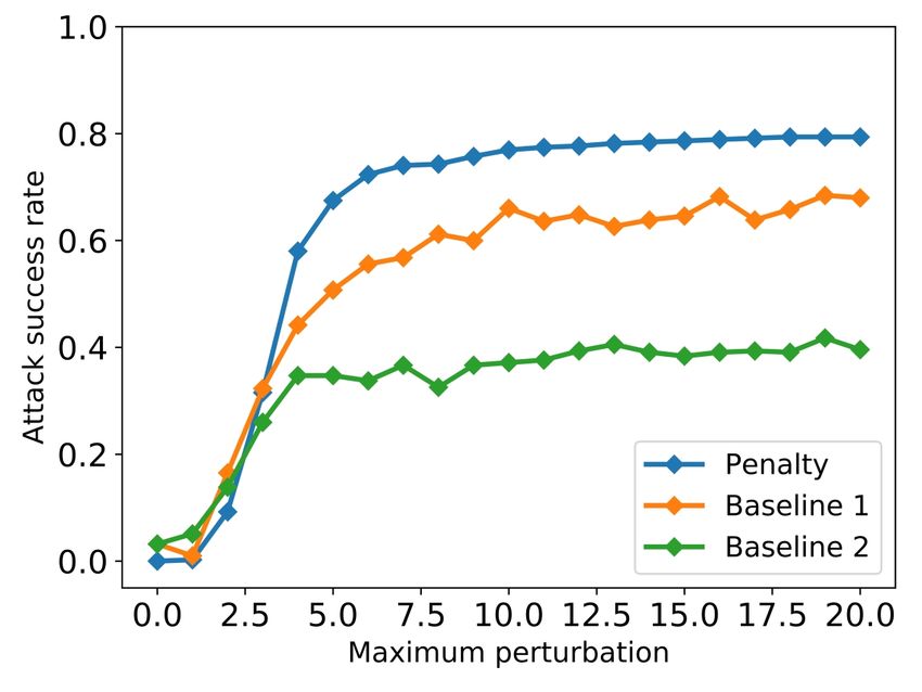
Feature                          Description
        NIP               Number of IPs contacting the domain
                                                                      added. We support other families of dependencies, among
    Num Conn                  Total number of connections             which one that has includes both statistical and ratio
    Avg Conn            Average number of connections by an IP        dependencies (see the definition of the ratio features for
 Total Sent Bytes              Total number of sent bytes             bytes sent over received). We omit here the details. The
 Total Recv Bytes            Total number of received bytes           important observation here is that the constraints update
 Avg Ratio Bytes    Average ratio bytes sent over received by an IP
 Min Ratio Bytes     Min ratio of bytes sent over received by an IP   functions are reusable across applications, and they can
 Max Ratio Bytes     Max ratio of bytes sent over received by an IP   be extended to support new mathematical dependencies.
    Frac empty      Fraction of connections with empty content type
     Frac html       Fraction of connections with html content type   Algorithm 3 Malicious Connection Classifier Attack
     Frac img       Fraction of connections with image content type
    Frac other      Fraction of connections with other content type   Require: x: data point in iteration m
                                                                       1: function UPDATE DEP(s, xm , ∇, Fimax )
TABLE 2: Example families of features (Connections,                    2:     if s == Stat then
Bytes, and Content) for malicious domains.                             3:         Update Stat(xm , ∇, Fimax )
                                                                       4:     if s == Ratio then
                                                                       5:         Update Ratio(xm , ∇, Fimax )
gregated port features is performed. The difference in the
                                                                       6: function Update Stat(xm , ∇, F )
total number of bytes sent by the attacker is determined
                                                                       7:     Parse F as: T (total number of events); N (number
from the gradient, followed by a projection operation to be
                                                                          of entities); XT , Xmin , Xmax , Xavg (the total, min,
within the feasible range for TCP and UDP packet sizes
                                                                          max, and average number of events per entity).
(function PROJECT). The PROJECT function takes an
                                                                       8:     // XT is representative feature.
input a value x and a range [a, b]. It projects x to the
                                                                       9:     XT0 ← Π(XT − α∇T )
interval [a, b] (if x ∈ [a, b], it returns x; if x > b, it                                     PN
returns b; otherwise it returns a). The duration is also set          10:     XN +1 ← XT0 − i=1 Xi
according to the gradient, again projecting based on lower            11:     Xmin ← min(Xmin , XN +1 )
and upper bounds computed from the data distribution.                 12:     Xmax ← max(Xmax , XN +1 )
The port family includes features such as Min and Max                 13:     N ← N + 1; XT ← XT0
sent bytes and connection duration. These need to be                  14: function Update Ratio(xm , ∇, F )
updated because we add new connections, which might                   15:     Parse FPas: N, Nr , X1 , . . . , XN such that: Xi =
                                                                                         N
include higher or lower values for sent bytes and duration.               Ni /N and i=1 Xi = 1.
    We assume that the attacker communicates with an                  16:     // Xr is representative feature
external IP under its control (for instance, the command-             17:     Nr0 ← Π(Nr − α∇r )
and-control IP), and thus has full control on the malicious           18:     N ← N + Nr0 − Nr
traffic. For simplicity, we set the number of received                19:     Xr ← Π(Nr0 /N )
packets and bytes to 0, assuming that the malicious IP                20:     Xi ← (dXi · N e)/N, ∀i 6= r
does not respond to these connections.                                21:     Nr ← Nr0

4.2. Malicious Domain Classifier                                      5. Experimental evaluation for malicious do-
                                                                      main classifier
Problem definition: dataset and features. The second
application is to classify domain names contacted by an                   One of the main challenges in evaluating our work
enterprise hosts as Malicious or Benign. We use a dataset             is the lack of standard benchmarks for security analytics.
from [51], that was collected by a company that includes              We first obtain access to a proprietary enterprise dataset
89 domain features extracted from HTTP proxy logs and                 from a security company, with features defined by domain
domain labels. The features come from 7 families, and we              experts. This dataset is based on real enterprise traffic,
include an example of several families in Table 2.                    includes labels of malicious domains, and is highly imbal-
Attack algorithm. In this application, we do not have                 anced. Secondly, we use a smaller public dataset (CTU-
access to the raw HTTP traffic, only to features extracted            13) to make our results reproducible. CTU-13 includes
from it. The majority of constraints are mathematical                 labeled Bro (Zeek) log connections for different botnet
constraints in the feature space. The attack algorithm                scenarios merged with legitimate campus traffic.
follows the framework from Algorithm 1, with the specific                 We first perform our evaluation on the enterprise
functions defined in Algorithm 3. The families of features            dataset, starting with a description of the dataset in Sec-
have various dependencies, as illustrated in the Connection           tion 5.1, ML model selection in Section 5.2, and evasion
and Content families. For Connection we have statistical              attack results in Section 5.3. We show initial results on
constraints (computing min, max, average values over                  adversarial training in Section 5.4.
a number of events), while for Content we have ratio
constraints (ensuring that the sum of all ratio values equals         5.1. Enterprise dataset
to 1). We assume that we add events to the logs (and never
delete or modify existing events). For instance, we can                   The data for training and testing the models was
insert more connections, as in the malicious connection               extracted from security logs collected by web proxies at
classifier. Function Update Stat shows how the statistical            the border of a large enterprise network with over 100,000
features are modified, while function Update Ratio shows              hosts. The number of monitored external domains in the
how the ratio features are modified if a new event is                 training set is 227,033, among which 1730 are classified as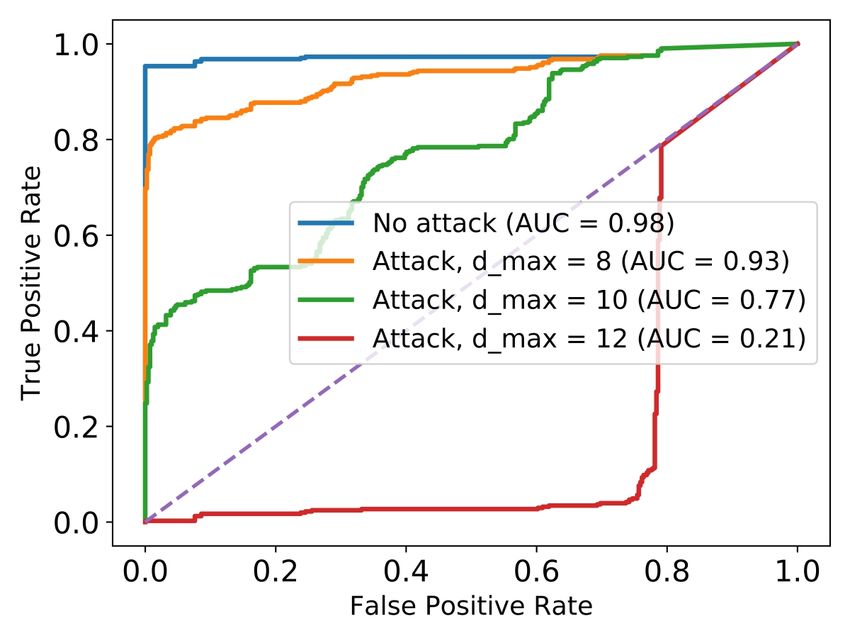
Malicious and 225,303 are Benign. For training, we sam-
pled a subset of training data to include 1230 Malicious
domains, and different number of Benign domains to get
several imbalance ratios between the two classes (1, 5,
15, 25, and 50). We used the remaining 500 Malicious
domains and sampled 500 Benign domains for testing the
evasion attack. Overall, the dataset includes 89 features
from 7 categories.
    We assume that the attacker controls the malicious
domain and all the communication from the victim ma-
chines to that domain, so it can change the commu-                       (a) Model comparison (balanced data).
nication patterns to the malicious domain. Among the
features included in the dataset, we determined a set
of 31 features that can be modified by an attacker (see
Table 15 in Appendix for their description). These include
communication-related features (e.g., number of connec-
tions, number of bytes sent and received, etc.), as well
as some independent features (e.g., number of levels in
the domain or domain registration age). Other features in
the dataset (for examples, those using URL parameters or
values) are more difficult to change, and we consider them
immutable during the evasion attack.                                             (b) Imbalance results.

5.2. Model Selection                                          Figure 4: Training results for malicious domain classifier.

Hyper-parameter selection. We first evaluate three stan-      of random forest, but it might be possible to improve
dard classifiers with different hyper-parameters (logis-      these results with additional effort (note that for higher
tic regression, random forest, and FFNN). The hyper-          imbalance ratio the performance of FFNN improves, as
parameters for logistic regression and random forests are     shown in Figure 4b). For the remainder of the section, we
in Tables 13 and 14 from the Appendix. For logistic           focus our discussion on the robustness of FFNN models.
regression, the maximum AUC score of 87% is achieved          Comparison of class imbalance for FFNN. Since the
with L1 regularization with inverse regularization 2.89.      issue of class imbalance is a known challenge in cyber
For random forest, the maximum AUC of 91% is ob-              security [7], we analyze the model accuracy as a function
tained with Gini Index criterion, maximum tree depth 13,      of imbalance ratio, showing the ROC curves in Figure 4b.
minimum number of samples in leaves 3, and minimum            Interestingly, the performance of the model increases to
samples for split 8.                                          93% AUC for imbalance ratio up to 25, after which it
    The architectures used for FFNN are illustrated in        starts to decrease (with AUC of 83% at a ratio of 50).
Table 3. The best performance was achieved with 2 hidden      Our intuition is that the FFNN model achieves better
layers with 80 neurons in the first layer, and 50 neurons     performance when more training data is available (up to
in the second layer. ReLU activation function is used after   a ratio of 25). But once the Benign class dominates the
all hidden layers except for the last layer, which uses       Malicious one (at ratio of 50), the model performance
sigmoid (standard for binary classification). We used the     starts to degrade.
Adam optimizer and SGD with different learning rates.
The best results were obtained with Adam and learning         5.3. Robustness to evasion attacks
rate of 0.0003. We ran training for 75 epochs with mini-
batch size of 32. As a result, we obtained the model with         After we train our models, we use a testing set of
AUC score 89% in cross-validation accuracy.                   500 Malicious and 500 Benign data points to evaluate the
                                                              evasion attack success rate. We vary the maximum allowed
         Hyperparameter                    Value
       Architecture 1 layer           [80], [64], [40]
                                                              perturbation expressed as an L2 norm and evaluate the
       Architecture 2 layers        [80, 60], [80, 50],       success of the attack. We evaluate the two optimization
                               [80, 40], [64, 32], [48, 32]   objectives for Projected and Penalty attacks and compare
       Architecture 3 layers            [80, 60, 40]          with several baselines. We also run directly the C&W
            Optimizer                   Adam, SGD
          Learning Rate                [0.0001, 0.01]
                                                              attack and show that it results in infeasible adversarial
                                                              examples (as expected). We evaluate the success rate of
      TABLE 3: DNN Architectures, epochs = 75                 the attacks for different imbalance ratios. We also perform
                                                              some analysis of the features that are modified by the
Model comparison. After performing model selection            attack, and if they correlate with feature importance. We
for each type of model, we compare the three best re-         show an adversarial example generated by our method
sulting models. Figure 4a shows the ROC curves and            and discuss how optimization-based attack performs under
AUC scores for a 1:1 imbalance ratio (with the same           weaker threat models.
number of Malicious and Benign points used in training).      Existing Attack. We run the existing C&W attack [14] on
The performance of FFNN is slightly worse than that           our data in order to measure if the adversarial examples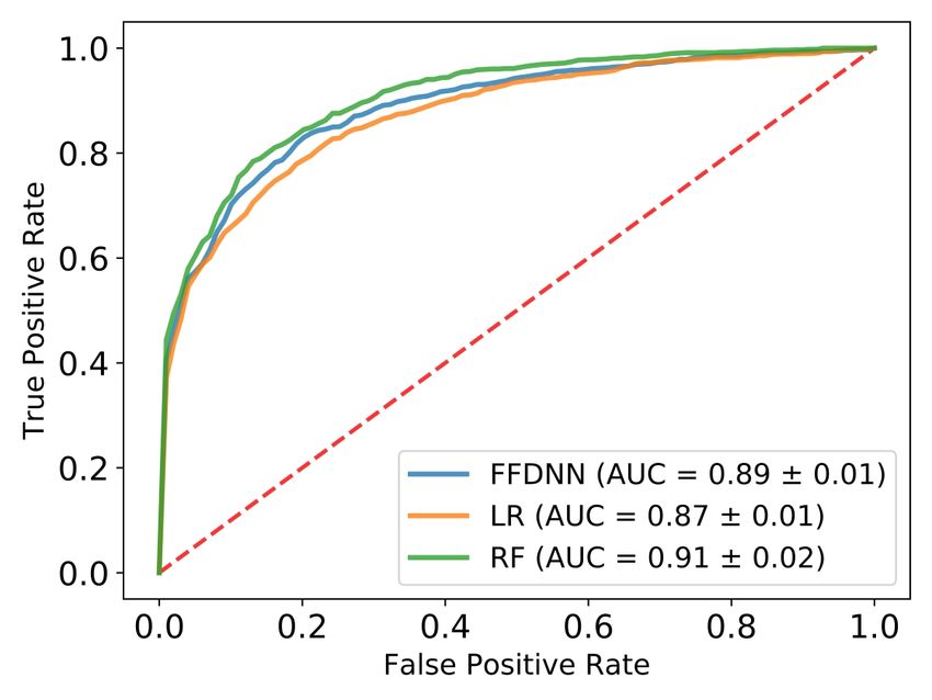
(a) Comparison to two baselines.         (b) ROC curves under attack.            (c) Imbalance sensitivity.
                                             Figure 5: Projected attack results.

are feasible. While the performance of the attack is high        experiment, we select 62 test examples which all models
and reaches 98% at distance 20 (for the 1:1 balanced case),      (trained for different imbalance ratios) classified correctly
the resulting adversarial examples are outside the feasibil-     before the evasion attack. The results are illustrated in
ity region. An example is included in Table 4, showing           Figure 5c. At L2 distance 20, the evasion attack achieves
that the average number of connections is not equal to           100% success rate for all ratios except 1. Additionally,
the total number of connections divided by the number of         we observe that with higher imbalance, it is easier for the
IPs. Additionally, the average ratio of received bytes over      attacker to find adversarial examples (at fixed distance).
sent bytes is not equal to maximum and minimum values            One reason is that models that have lower performance
of ratio (as it should be when the number of IPs is 1).          (as the one trained with 1:50 imbalance ratio) are easier
                                                                 to attack. Second, we believe that as the imbalance gets
        Feature        Input   Adversarial   Correct Value       higher the model becomes more biased towards the major-
                                Example
         NIP             1          1             1
                                                                 ity class (Benign), which is the target class of the attacker,
       N Conn           15       233.56         233.56           making it easier to cross the decision boundary between
      Avg Conns         15        59.94         233.56           classes.
    Avg Ratio Bytes    8.27      204.01         204.01
    Max Ratio Bytes    8.27      240.02         204.01
                                                                 Penalty attack results. We now discuss the results
    Min Ratio Bytes    8.27      119.12         204.01           achieved by applying our attack with the Penalty objective
                                                                 on the testing examples. Similar to the Projected attack,
TABLE 4: Adversarial example generated by C&W. The               we compare the success rate of the Penalty attack to the
example is not consistent in the connection and ratio of         two types of baseline attacks (for balanced classes), in Fig-
bytes features, as highlighted in red. The correct value is      ure 6a (using the 412 Malicious testing examples classified
shown for a feasible example in green.                           correctly). Overall, the Penalty objective is performing
                                                                 worse than the Projected one, reaching 79% success rate
Projected attack results. We evaluate the success rate           at L2 distance of 20. We observe that in this case both
of the attack with Projected objective first for balanced        baselines perform worse, and the attack improves upon
classes (1:1 ratio). We compare in Figure 5a the attack          both baselines significantly. The decrease of the model’s
against two baselines: Baseline 1 (in which the features         performance under the Penalty attack is illustrated in
that are modified iteratively are selected at random), and       Figure 6b (for 500 Malicious and 500 Benign testing
Baseline 2 (in which, additionally, the amount of per-           examples). While AUC is 0.87 originally on the testing
turbation is sampled from a standard normal distribution         dataset, it decreases to 0.59 under the evasion attacks
N (0, 1)). The attacks are run on 412 Malicious testing          at maximum allowed perturbation of 7. Furthermore, we
examples classified correctly by the FFNN. The Projected         measure the attack success rate at different imbalance
attack improves both baselines, with Baseline 2 perform-         ratios in Figure 6c (using the 62 testing examples clas-
ing much worse, reaching success rate 57% at distance            sified correctly by all models). For each ratio value we
20, and Baseline 1 having success 91.7% compared to              searched for the best hyper-parameter c between 0 and
our attack (98.3% success). This shows that the attacks          1 with step 0.05. Here, as with the Projected attack, we
is still performing reasonably if feature selection is done      see the same trend: as the imbalance ratio gets higher,
randomly, but it is very important to add perturbation to        the attack performs better, and it works best at imbalance
features consistent with the optimization objective.             ratio of 50.
    We also measure in Figure 5b the decrease of the             Attack comparison. We compare the success rate of our
model’s performance before and after the evasion attack          attack using the two objectives (Projected and Penalty)
at different perturbations (using 500 Malicious and 500          with the C&W attack, as well as an attack we call Post-
Benign examples not used in training). While AUC score           processing. The Post-processing attack runs directly the
is 0.87 originally, it drastically decreases to 0.52 under       original C&W developed for continuous domains, after
evasion attack at perturbation 7. This shows the significant     which it projects the adversarial example to the feasible
degradation of the model’s performance under evasion             space to enforce the constraints. In the Post-processing
attack.                                                          attack, we look at each family of dependent features, keep
    Finally, we run the attack at different imbalance ratios     the value of the representative feature as selected by the at-
and measured its success for different perturbations. In this    tack, but then modify the values of the dependent features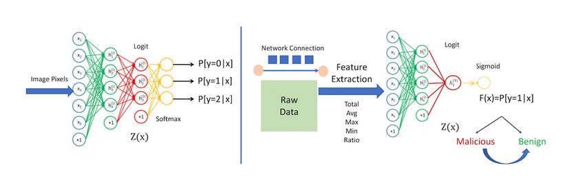
(a) Comparison to two baselines.        (b) ROC curves under attack.            (c) Imbalance sensitivity.
                                             Figure 6: Penalty attack results.

                                                                axis) and feature importance (right axis). We observe that
                                                                features of higher importance are chosen more frequently
                                                                by the optimization attack. However, since we are modify-
                                                                ing the representative feature in each family, the number
                                                                of modifications on the representative feature is usually
                                                                higher (it accumulates all the importance of the features
                                                                in that family). For the Bytes family, feature 3 (number
                                                                of received bytes) is the representative feature and it is
                                                                updated more than 350 times. However, for features that
                                                                have no dependencies (e.g., 68 – number of levels in
                                                                the domain, 69 – number of sub-domains, 71 – domain
      Figure 7: Malicious domain classifier attacks.            registration age, and 72 – domain registration validity), the
                                                                number of updates corresponds to the feature importance.
                                                                               Feature       Original    Adversarial
                                                                                 NIP            1             1
using the UPDATE DEP function. The success rate of all                    Total Recv Bytes    32.32       43653.50
these attacks is shown in Figure 7, using the 412 Malicious               Total Sent Bytes     2.0         2702.62
testing examples classified correctly. The attacks based                  Avg Ratio Bytes     16.15         16.15
on our framework (with Projected and Penalty objectives)                  Registration Age     349          3616
perform best, as they account for feature dependencies          TABLE 5: Adversarial example for the Projected attack
during the adversarial point generation. The attack with        (distance 10).
the Projected objective has the highest performance (we
suspect that the Penalty attack is sensitive to parameter       Adversarial examples. We include an adversarial exam-
c). The vanilla C&W has slightly worse performance at           ple in Table 5 for the Projected attack. We only show the
small perturbation values, even though it does not take         features that are modified by the attack and their original
into consideration the feature constraints and works in an      value. As we observe, the attack preserves the feature
enlarged feature space. Interestingly, the Post-processing      dependencies: the average ratio of received bytes over
attack performs worse (reaching only 0.005% success             sent bytes (Avg Ratio Bytes) is consistent with number of
at distance 20 – can generate 2 out of 412 adversarial          received (Total Recv Bytes) and sent (Total Sent Bytes)
examples). This demonstrates that it is not sufficient to       bytes. In addition, the attack modifies the domain regis-
run state-of-art attacks for continuous domains and then        tration age, an independent feature, relevant in malicious
adjust the feature dependencies, but more sophisticated         domain classification [47]. However there is a higher
attack strategies are needed.                                   cost to change this feature: the attacker should register
Number of features modified. We compare the number              a malicious domain and wait to get a larger registration
of features modified during the attack iterative algorithm      age. If this cost is prohibitive, we can easily modify our
to construct the adversarial examples for three attacks:        framework to make this feature immutable (see Table 15
Projected, Penalty, and C&W. The histogram for the num-         in Appendix for a list of features that can be currently
ber of modified features is illustrated in Figure 8a. It is     modified by the attack).
not surprising that the C&W attack modifies almost all          Weaker attack models. We consider a threat model
features, as it works in L2 norms without any restriction in    in which the adversary only knows the feature repre-
feature space. Both the Projected and the Penalty attacks       sentation, but not the exact ML model or the training
modify a much smaller number of features (4 on average).        data. One approach to generate adversarial examples is
    We are interested in determining if there is a relation-    through transferability [52], [46], [68], [64], [21]. We
ship between feature importance and choice of feature           perform several experiments to test the transferability of
by the optimization algorithm. For additional details on        the Projected attacks against FFNN to logistic regression
feature description, we include the list of features that       (LR) and random forest (RF). Models were trained with
can be modified in Table 15 in the Appendix. In Figure 8b       different data and we vary the imbalance ratio. The results
we plot the number of modifications for each feature (left      are in Table 6. We observe that the largest transferability
(a) Histogram on feature modifications. (b) Number of updates (left) and feature importance (right).
Figure 8: Feature statistics.
rate to both LR and RF is for the highest imbalanced other more effective methods of performing black-box
ratio of 50 (98.2% adversarial examples transfer to LR attacks in future work.
and 94.8% to RF). As we increase the imbalance ratio,
the transfer rate increases, and the transferability rate to 5.4. Adversarial Training
LR is lower than to RF.
Finally, we looked at defensive approaches to protect
Ratio DNN LR RF
1 100% 40% 51.7% ML classifiers in security analytics tasks. One of the most
5 93.3% 66.5% 82.9% robust defensive technique against adversarial examples
15 99% 60.9% 90.2% is adversarial training [29], [48]. We trained FFNN us-
25 100% 47.6% 68.8% ing adversarial training with the Projected attack at L2
50 100% 98.2% 94.8%
distance 20. We trained the model adversarially for 11
TABLE 6: Transferability of adversarial examples from epochs and obtain AUC score of 89% (each epoch takes
FFNN to LR (third column) and RF (fourth column). We approximately 7 hours). We measure the Projected attack’s
vary the ratio of Benign to Malicious in training. Column success rate for the balanced case against the standard
FFNN shows the white-box attack success rate. and adversarially training models in Figure 9. Interest-
ingly, the success rate of the evasion attacks significantly
We also look at the transferability between different drops for the adversarially-trained model and reaches only
FFNN architectures trained on different datasets (results 16.5% at 20 L2 distance. This demonstrates that adversar-
in Table 7). The attacks transfer best at highest imbalance ial training is a promising direction for designing robust
ratio (with success rate higher than 96%), confirming that ML models for security.
weaker models are easier to attack.
Ratio DNN1 DNN2 DNN3
[80, 50] [160, 80] [100, 50, 25]
1 100% 57.6% 42.3%
5 93.3% 73.6% 58.6%
15 99% 78.6% 52.4%
25 100% 51.4% 45.3%
50 100% 96% 97.1%
TABLE 7: Transferability between different FFNN archi-
tectures (number of neurons per layer in the second row).
Adversarial examples are computed against DNN1 and
transferred to DNN2 and DNN3.
Figure 9: Success rate of the Projected attack against
adversarially and standard trained model.
Alternative approaches to perform black-box attacks
is to use substitute model and synthetic training inputs la-
beled by the target classifier using black-box queries [53]
or to query the ML classifier and estimate gradient val- 6. Experimental evaluation for malicious
ues [37]. Running directly existing black-box attacks
does not generate feasible adversarial examples, thus we
connection classifier
adapted the black-box attack of Ilyas et al. [37] to our
setting (assuming the attacker knows the feature represen- Hyperparameter Value
tation). When estimating the gradient of the attacker’s loss Architecture [256, 128, 64]
Optimizer Adam
function, we use finite difference that incorporates time- Learning Rate 0.00026
dependent information and perform our standard proce-
dure of updating feature dependencies. The attack success TABLE 8: DNN Architecture
is only 28.4% (with 48 queries). We plan to investigate(a) Projected attack success rate. (b) ROC curves under attack. (c) Average number of updated ports.
Figure 10: Projected attack results on malicious connection classifier.
Training scenario F1 AUC
1, 2 0.94 0.96
6.2. Classification results
1, 9 0.96 0.97
2, 9 0.83 0.79 We perform model selection and training for a number
of FFNN architectures on all combinations of two sce-
TABLE 9: Training results for FFNN. narios, and tested the models for generality on the third
scenario. The best architecture is illustrated in Table 8.
Feature Input Delta Adversary
Total TCP 6809 12 6821 It consists of three layers with 256, 128 and 64 hidden
Total Sent Pkts 29 1044 1073 layers. We used the Adam optimizer, 50 epochs for train-
Max Sent Pkts 11 76 87 ing, mini-batch of 64, and a learning rate of 0.00026.
Sum Sent Bytes 980 1348848 1349828 The F1 and AUC scores for all combinations of training
Max Sent Bytes 980 111424 112404
Total Duration 2.70 5151.48 5154.19
scenarios are illustrated in Table 9. We also compared the
Max Duration 2.21 430.26 432.47 performance of FFNN with logistic regression and random
forest, but we omit the results (FFNN achieved similar
TABLE 10: Feature statistics update when generating an performance to random forest). For the adversarial attacks,
adversarial example at distance 14, on port 443. we choose the scenarios with best performance: training
on 1, 9, and testing on 2.
In this application we have access to raw network
6.3. Robustness to evasion attacks
connections (in Bro log format), which provides the op-
portunity to generate feasible adversarial examples in both We show the Projected attack’s performance, discuss
feature representation and raw data space. We show how which ports were updated most frequently, and show
an attacker can insert new realistic network connections an adversarial examples and the corresponding Bro logs
to change the prediction of Malicious activity. We only records. The testing data for the attack is 407 Malicious
analyze the Projected attack here, as it demonstrated best examples from scenario 2, among which 397 were pre-
performance in the previous application. The code of the dicted correctly by the classifier.
attack and the dataset are available at https://github.com/
achernikova/cybersecurity evasion. The malicious domain Evasion attack performance. First, we analyze the attack
dataset is proprietary and we cannot release it. success rate with respect to the allowed perturbation,
shown in Figure 10a. The attack reaches 99% success
We start with a description of the CTU-13 dataset
rate at L2 distance 16. Interestingly, in this case the
in Section 6.1, then we show the performance of FFNN
two baselines perform poorly, demonstrating again the
for connection classification in Section 6.2. Finally, we
clear advantages of our framework. We plot next the
present the analysis on model robustness in Section 6.3.
ROC curves under evasion attack in Figure 10b (using
the 407 Malicious examples and 407 Benign examples
6.1. CTU-13 dataset from testing scenario 2). At distance 8, the AUC score
is 0.93 (compared to 0.98 without adversarial examples),
CTU-13 is a collection of 13 scenarios including both but there is a sudden change at distance 10, with AUC
legitimate traffic from a university campus network, as score dropping to 0.77. Moreover, at distance 12, the
well as labeled connections of malicious botnets [27]. AUC reaches 0.12, showing the model’s degradation under
We restrict to three scenarios for the Neris botnet (1, evasion attack with relatively small distance.
2, and 9). We choose to train on two of the scenarios Ports family statistics. We show the average number of
and test the models on the third, to guarantee indepen- port families updated during the attack in Figure 10c. The
dence between training and testing data. The training data maximum number is 3 ports, but it decreases to 1 port at
has 3869 Malicious examples, 194,259 Benign examples, distance higher than 12. While counter-intuitive, this can
and an imbalance ratio of 1:50. There is a set of 432 be explained by the fact that at larger distances the attacker
statistical features that the attacker can modify (the ones can add larger perturbation to the aggregated statistics of
that correspond to the characteristics of sent traffic). The one port, crossing the decision boundary.
physical constraints and statistical dependencies on bytes In Table 12 we include the port families selected
and duration have been detailed in Section 4.1. during attack, at distance 8, as well as their importance.You can also read