All that glitters is not gold. Influence of working from home on income inequality at the time of Covid-19 - INAPP WP n. 50 - oa inapp

WORKING PAPER

INAPP WP n. 50

All that glitters is not gold. Influence
of working from home on income
inequality at the time of Covid-19
Luca Bonacini
Giovanni Gallo
Sergio Scicchitano

GIUGNO 2020

All that glitters is not gold. Influence
of working from home on income
inequality at the time of Covid-19

Luca Bonacini
Università degli studi di Modena e Reggio Emilia (UNIMORE), Modena, Reggio Emilia
luca.bonacini@unimore.it

Giovanni Gallo
Università degli studi di Modena e Reggio Emilia, (UNIMORE), Modena, Reggio Emilia
Istituto nazionale per l’analisi delle politiche pubbliche (INAPP), Roma
gi.gallo.ext@inapp.org

Sergio Scicchitano
Istituto nazionale per l’analisi delle politiche pubbliche (INAPP), Roma
s.scicchitano@inapp.org

GIUGNO 2020

We thank Gaetano Basso Irene Brunetti, and Mauro Caselli for useful comments. The views
expressed in this paper are those of the authors and do not necessarily reflect those of INAPP.

CONTENTS: 1. Introduction. – 2. Data. – 3. Methodology and model specifications. – 4. Results; 4.1
Descriptive evidences; 4.2 Kolmogorov-Smirnov test; 4.3 Influences of occupations attitude
towards working from home. – 5. Robustness checks. – 6. Conclusions. – Appendix. – References

 INAPP – Istituto nazionale per l’analisi delle politiche pubbliche
 Corso d’Italia 33 Tel. +39 06854471
 00198 Roma, Italia Email: urp@inapp.org www.inapp.org

ABSTRACT

All that glitters is not gold. Influence
of working from home on income
inequality at the time of Covid-19
The recent global Covid-19 pandemic forced most of governments in developed countries
to introduce severe measures limiting people mobility freedom in order to contain the
infection spread. Consequently, working from home (WFH) procedures became of great
importance for a large part of employees, since they represent the only option to both
continue working and keep staying home. Based on influence function regression
methods, our paper explores the role of WFH attitude across labour income distribution
in Italy. Results show that increasing WFH attitudes of occupations would lead to a rise of
wage inequality among Italian employees. Specifically, a change from low to high WFH
attitude would determine a 10% wage premium on average and even higher premiums
(+17%) in top deciles of wage distribution. A possible improvement of occupations WFH
attitude tends to benefit male, older and high-paid employees, as well as those living in
provinces more affected by the novel coronavirus.

KEYWORDS: Covid-19, working from home, inequality, unconditional quantile regressions

JEL CODES: D31, I18, J16

4 All that glitters is not gold. Influence of working from home on income inequality at the time of Covid-19

 “That push [related to reopening decisions during the pandemic] is likely to exacerbate longstanding
 inequalities, with workers who are college educated, relatively affluent and primarily white able to continue
 working from home and minimizing outdoor excursions to reduce the risk of contracting the virus”

 The New York Times, April 27 20201

1. Introduction

The Covid-19 pandemic is raging worldwide, and it probably does not run out in the short term, thus
causing possible structural effects on the labour market in many countries (Baert et al. 2020a). The
contagion speed of the coronavirus seems to be also favoured by globalization (Zimmermann et al.
2020). Most of governments in developed countries responded by suspending many economic
activities and limiting people mobility freedom (Baldwin and Weder di Mauro 2020; Qiu et al. 2020;
Flaxman et al. 2020). In this context, the working from home (WFH) procedures became of great
importance, since they allow to continue working and thus receiving wages (as for employees), to
keep producing services and revenues (as for employers), and to overall limit the infection spread risk
and pandemic recessive impacts in the country. Due to the uncertainty about the actual pandemic
duration or future contagion waves, the role of WFH in the labour market is further emphasized by
the fact that it might become a traditional (rather than unconventional) way of working in many
economic sectors (Alon et al. 2020). It has been recently found that the great majority of the
employees in Belgium believe that teleworking (85%) and digital conferencing (81%) will continue
after the SARS-CoV-2 crisis (Baert et al. 2020b).
Because of its sudden prominence growth, several studies recently investigated the WFH
phenomenon. Most of these studies (see, for instance, Béland et al. 2020; Dingel and Neiman 2020;
Gottlieb et al. 2020; Hensvik et al. 2020; Holgersen et al. 2020; Koren and Peto 2020; Leibovici et al.
2020; Yasenov 2020) aim to classify occupations according to their WFH attitude in the US and some
European countries (e.g. UK, Germany) and in Latin American and Caribbean countries (Delaporte and
Peña 2020). As for Italy Boeri et al. (2020), starting from the U.S. O*NET dataset, estimate that 24% of
jobs can be carried out from home, while Barbieri et al. (2020) build an indicator of the WFH attitude
for sectors and occupations. Just few of them instead deepen on employees’ characteristics, showing
that WFH attitude in the US, UK and Germany is lower among less educated and overall low-paid
workers (Adams-Prassl et al. 2020; Mongey et al. 2020)2. However, the literature still neglects
potential effects of WFH along the wage distribution and on income inequality in general.
This paper aims to provide some first insights on the role of WFH on labour income inequality.
Specifically, using the influence function regression method proposed by Firpo et al. (2009), we

1
 See: https://rb.gy/3qzyj0.
2
 Working from home has already been studied in normal times (e.g. Blinder and Krueger 2013; Bloom et al.
2015). Some articles evaluated the effect of flexible work practices on wages (Weeden 2005; Gariety and Shaer
2007; Leslie et al. 2012; Arntz et al. 2019; Pabilonia and Vernon 2020). Pigini and Staffolani (2019) estimate the
average wage premium of telework in Italy. Angelici and Profeta (2020) in a randomized experiment among
Italian workers show that flexibility of working from home can reduce gender disparities.

All that glitters is not gold. Influence of working from home on income inequality at the time of Covid-19 5

estimate the unconditional effect along the wage distribution of a marginal change in the WFH
attitude. To do that, we focus on Italy as an interesting case study, because both it is one of the
countries most affected by the novel coronavirus and it was the first Western country to adopt a
lockdown of economic activities (on March 25). Barbieri et al. (2020) estimated that further 3 million
of employees (i.e. about 13% of total) started to work from home because of this companies-
lockdown, but a large part started even earlier because of both the schools-lockdown (on March 5)
and the national quarantine (on March 12) (more details in Bonacini et al. 2020).
We use a uniquely detailed dataset relying on the merge of two sample surveys. The first one is the
Survey on Labour Participation and Unemployment (i.e. Inapp PLUS) for the year 2018, which contains
information on incomes, education level, and employment conditions of working age Italians. The
second sample survey is the Italian Survey of Professions (ICP) for the year 2013, which provides
detailed information of the task-content of occupations at the 5-digit ISCO classification level. ICP is
the Italian equivalent of the US O*NET repertoire and it allows us to build the WFH attitude index
recently proposed by Barbieri et al. (2020). With respect to Boeri et al. (2020) who report the number
of employees suitable for working from home in Italy, a key point of our data is therefore that our task
and skill variables directly refer to the Italian labour market. Finally, we merge our dataset to the one
provided by the Italian Civil Protection Department (2020) for the period February 24-May 5 2020 to
investigate to what extent the WFH attitude influence on labour income distribution is higher in
provinces most affected by the novel coronavirus.

2. Data

Data we use in this article are from an innovative dataset recently built by merging two Italian surveys,
developed and administered by the National Institute for Public Policy Analysis (Inapp). The first one
is the Participation, Labour and Unemployment Survey (PLUS), which is able to provide reliable
statistical estimates of labour market phenomena that are rare or marginally explored by the Labour
Force Survey. It also provides a wide range of standard individual characteristics, as well as numerous
characteristics related to his job and firm, for approximately 45,000 individuals in each wave. We use
the last Eighth wave of the Survey, which was collected in 2018 and released in the first half of 2019.
A dynamic computer-assisted telephone interview (i.e. a CATI interview) was used to contact
participants. One of the key elements of this dataset is the absence of proxy interviews: in the survey,
only survey respondents are reported, to reduce measurement errors and partial non-responses. The
questionnaire was distributed to a sample of residents aged between 18 and 74 according to a
stratified random sampling over the Italian population3. The Inapp PLUS survey also provides
individual weights to account for non-response and attrition issues which usually affect sample
surveys. Similarly to other empirical studies relying on the same dataset (see, among others, Clementi
and Giammatteo 2014; Filippetti et al. 2019; Meliciani and Radicchia 2011, 2016; Van Wolleghem et

3
 The stratification of the Inapp PLUS survey sample is based on population strata by NUTS-2 Region of residence,
urbanisation degree (i.e., metropolitan or non-metropolitan area), age group, sex, and employment status (i.e.,
employed, unemployed, student, retired, or other inactive status).

6 All that glitters is not gold. Influence of working from home on income inequality at the time of Covid-19

al. 2019; Esposito and Scicchitano 2020), all descriptive statistics and estimates reported in this
analysis are weighted using those individual weights.
The second one is the 2013 wave of the Italian Sample Survey on Professions (ICP), created in 2004
and currently carried out by Inapp. The ICP integrates the traditional approach by focusing on nature
and content of the work. It aims to describe, with a high analytical detail, all existing professions both
in terms of requirements and characteristics required of the worker, both in terms of activities and
working conditions that the profession implies. It was chosen to involve workers rather than experts,
privileging the point of view of those who exercise daily professions under study and have a direct and
concrete assessment of the level of use of certain characteristics essential to carry out one's job. The
survey reports information on about 16,000 workers and describes all the 5-digit occupations (i.e. 811
occupational codes) existing in the Italian labour market, from those operating in private companies
to those present within the institutions and public structures, up to those operating under autonomy.
The conceptual reference framework for the investigation and the taxonomies of variables used are
borrowed from the US model of the Occupational Information Network, O*Net. It is the most
complete from the point of view of the job description, being also able to respond simply and
comprehensively to potentials stakeholder questions. Thus the questions refer to the US O*Net
conceptual model, according to which the profession is a multi-dimensional concept that can be
described referring to the following thematic areas: a) worker requirements: skills, knowledge,
educational level; b) worker characteristics: skills, values, working styles; c) profession requirements:
generalized work activities, working context; d) experience requirements: training, experience.
Remarkably, Italy is one of the few European countries to have a dictionary of occupations similar to
the US O*NET. Thus, being the ICP based on Italian occupations and not on those of the US, it is able
to capture the specific features of the Italian productive structure, which the O*NET is not able to
grasp thus avoiding potential biases. The existing literature (Boeri et al. 2020) use instead US O*Net
data and crosswalks between US and Italy, which possibly reflect US-specific technology adoption and
labour market structure.
The ICP survey includes questions that are particularly relevant to evaluate the attitude to smart-
working of workers in the current Covid-19 emergency. More specifically, we use WFH attitude index
recently proposed by Barbieri et al. (2020), which is calculated for each 5-digit occupation and goes
from a 0 to 100 scale (from less to more intense). The composite index is computed by taking the
average of the following seven questions: (i) importance of working with computers; (ii) importance
of performing general physical activities (which enters with reversely); (iii) importance of manoeuvring
vehicles, mechanical vehicles or equipment (reversely); (iv) requirement of face-to-face interactions
(reversely); (v) dealing with external customers or with the public (reversely); (vi) physical proximity
(reversely); (vii) time spent standing (reversely). The index was aggregated at the ISCO 4-digits level to
merge it with PLUS.
From the total Inapp PLUS sample, to develop our analysis, we drop people with no occupation (e.g.
students, retires, unemployed). We also drop self-employed from our sample, because of their
potentially strong heterogeneity and unclarity in the usage of working from home procedures. Finally,
we drop observations with missing values in relevant variables and we apply a usual age restriction,
selecting only employees aged 25-64 years old. Our analysis sample of employees therefore counts
14,307 observations.

All that glitters is not gold. Influence of working from home on income inequality at the time of Covid-19 7

3. Methodology and model specifications

Formally, let be the distribution function of gross labour incomes and ( ) denote a distributional
statistic, such as the mean or a quantile. Since we can identify two categories of employees in terms
of WFH attitude, can be expressed as

 ( ) = 1 1 ( ) + 2 2 ( ) (1)

where is the gross labour income (i.e. the outcome variable), 1 ( 2 ) is the income distribution
among employees with low (high) WFH attitude, and 1 ( 2) is the share of employees in that subgroup
on the total sample.
Firpo et al. (2009) proposed a methodology to estimate the impact of marginal changes in the
distribution of interest variables on the distributional statistic ( ). Following Choe and Van Kerm
(2018), we label this measure as ‘unconditional effect’ (UE). Firpo et al. (2009) demonstrate that
 ( ( ), 2) can be also expressed as

 UE( ( ), 2) = ∫ RIF( ; , ) ( 1 , ,2 − )( ) (2)

where 1 , ,2 is the gross income distribution after the marginal substitution of employees, i.e.
 1 , ,2 = ( 2 + ) 2 ( ) + ( 1 − ) 1 ( ), RIF( ; , ) = ( ) + IF( ; , ) is the recentered
influence function of ( ) and

 ((1 − ) + ∆ ) − ( )
 IF( ; , ) = lim (3)
 ↓0 

is the influence function introduced by Hampel (1974). According to Firpo et al. (2009), the UEs can
be correctly calculated through a simple OLS estimation. Once the values of RIF( ; , ) are computed
for all observations for the distributional statistic ( ), they are regressed by OLS on our variable of
interest. The latter is defined as a dummy taking value 1 for employees with a high level of WFH
attitude, thus a value of the indicator proposed by Barbieri et al. (2020) over the sample median (i.e.
52.2), and 0 otherwise.
The unconditional quantile regression method also allows for taking into account demographic and
economic characteristics which may differ across employees, leading to potential biases on policy
influences. To this end, RIFs must be regressed through an OLS model including a vector of relevant
covariates beyond the variable of interest. The resulting effect is labelled as ‘unconditional partial
effect’ (UPE) (Firpo et al. 2009; Choe and Van Kerm 2018), but it is also named ‘policy effect’ (Rothe
2010; Gallo and Pagliacci 2020). UPEs are formally defined as

 UPE( ( ), ) = (∫ E[IF( ; , )| = , = ) − E[IF( ; , )| = 1, = ] ( ) ) × (4)
 
here denotes a set of employees given the covariates vector . Following Firpo et al. (2009), we
set the ‘attitude shift’ to 1 in order to estimate the UEs and UPEs. This means that influence estimates
on labour income distribution assume that all employees reporting low levels of WFH attitude increase
their attitude until becoming employees with a high WFH one. Although this assumption may appear

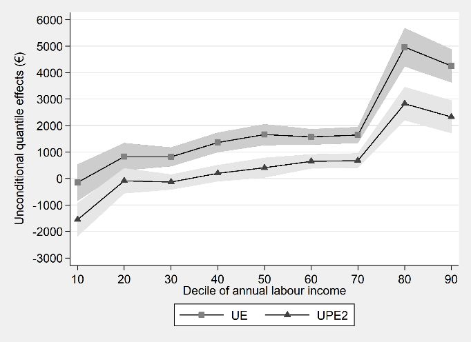
8 All that glitters is not gold. Influence of working from home on income inequality at the time of Covid-19

of difficult application, it remains however plausible for most of occupations with low WFH attitude
given both the limited threshold to overpass (i.e. 52.2 out of 100) and the fact that the WFH attitude
indicator is multidimensional. In fact, even if a dimension of the WFH attitude indicator is
unchangeable, maybe there are margins of improvement in the other six dimensions (see section 2
for details on the adopted indicator of WFH attitude). Of course, in the adopted methodological
framework, the counterfactual scenario is represented by the starting situation, thus assuming no
change in WFH attitude of occupations.
In this study, we estimate influences of a change in WFH attitude on gross labour income distribution
focusing on the following distributional statistics: the mean, the Gini index, and the nine deciles4.
Sample values of first two statistics are reported in section 4.1, while values of the nine deciles are
presented in figure A.1. As for the UPEs estimation, given the potential endogeneity of job
characteristics on the dependent variable, we consider two different vectors of covariates. The first
one (UPE1) includes only demographic characteristics regarding the individual and her household (i.e.
gender, age group, education level, migration status, marital status, household size, presence of
minors, municipality size, and macro-region of residence). The second vector of covariates (UPE2) also
adds job characteristics (i.e. job contract, public servant, and activity sector dummies), which may
determine potential endogeneity issues. More details on variables are provided in table A1.
Differently from the common choice to drop female employees to minimize selection issues, we
decided not to restrict the sample to males only but to show separated results by males and females.
To further explore the heterogeneous influences of an overall increase of WFH attitude along labour
income distribution, we also report main results distinguishing by age group and the extent of Covid-
19 infection at provincial (NUTS-3) level as reported by the Italian Civil Protection Department (2020).
All descriptive statistics and estimates consider individual sample weights. As a sensitivity analysis, to
control for the occupation skill heterogeneity among employees, we estimated our main results using
a set of covariates including skill level dummies (see section 5). We also controlled for potential
endogeneity related to the WFH attitude, developing other robustness checks on different inequality
indicators, sample selections, and scaled estimates. Their results, provided in section 5, overall confirm
the robustness of our main considerations.

4. Results

4.1 Descriptive evidences
Preliminary evidences about the sample composition, values of mean and Gini index of annual labour
income, mean value of the WFH attitude index and share of employees with high attitude level by
group of employees are shown in table 15.

4
 For the sake of brevity, formulas to calculate the RIFs for the mean, the Gini index, and the quantiles are not
replicated here, but they can be easily found in Choe and Van Kerm (2018).
5
 The same information is also provided by activity sector in which employees work in table A2.

All that glitters is not gold. Influence of working from home on income inequality at the time of Covid-19 9

Table 1. Sample composition, mean and Gini index of annual labour income, mean value of the WFH
 attitude index and share of employees with high attitude level by group of employees
 Sample composition Annual labour income WFH attitude
 % of
Variable employees
 Mean Std. Dev. Mean Gini index Mean
 with high
 attitude
Low WFH attitude 0.518 0.500 24,731 0.261 40.5 0.0
High WFH attitude 0.482 0.500 27,320 0.296 65.1 100.0
Male 0.537 0.499 29,321 0.283 52.3 45.3
Female 0.463 0.499 22,098 0.256 52.5 51.5
Aged 25-35 0.204 0.403 21,962 0.257 51.7 46.9
Aged 36-50 0.467 0.499 26,146 0.279 52.5 47.9
Aged 51-64 0.329 0.470 28,232 0.282 52.5 49.4
Lower secondary education (or lower) 0.313 0.464 23,500 0.284 46.7 27.4
Upper secondary education 0.464 0.499 25,670 0.267 54.6 54.7
Tertiary education 0.224 0.417 30,082 0.277 55.8 63.7
Local 0.882 0.322 25,912 0.276 52.4 48.4
Migrant within macro-region 0.031 0.173 28,434 0.360 53.2 52.1
Migrant within country 0.066 0.248 26,839 0.276 52.8 51.5
Foreign migrant 0.021 0.143 22,429 0.306 48.2 22.8
Unmarried 0.429 0.495 24,045 0.261 52.3 47.6
Married 0.571 0.495 27,432 0.290 52.4 48.6
Household size = 1 0.141 0.348 26,961 0.269 53.4 48.9
Household size = 2 0.202 0.401 25,973 0.284 52.1 48.1
Household size = 3 0.283 0.450 24,772 0.258 52.5 48.8
Household size = 4 0.291 0.454 26,574 0.289 52.6 49.0
Household size = 5 or more 0.083 0.276 26,349 0.325 50.1 42.3
Absence of minors 0.657 0.475 25,770 0.285 52.4 48.4
Presence of minors 0.343 0.475 26,378 0.270 52.4 47.7
Very small municipality 0.206 0.404 25,394 0.270 50.9 41.4
Small municipality 0.329 0.470 26,376 0.285 51.5 45.2
Medium municipality 0.159 0.366 25,668 0.269 52.3 48.1
Big municipality 0.167 0.373 26,196 0.300 53.1 52.6
Metropolitan city 0.139 0.346 25,998 0.269 55.9 60.3
North 0.538 0.499 26,666 0.267 52.4 47.1
Center 0.214 0.410 24,911 0.267 53.6 53.2
South 0.248 0.432 25,410 0.317 51.3 46.1
Full-time open-ended worker 0.695 0.461 29,225 0.240 53.0 48.9
Part-time open-ended worker 0.153 0.360 17,527 0.293 52.7 52.7
Temporary worker and other 0.152 0.359 19,659 0.310 49.4 40.3
Private sector employee 0.700 0.458 25,443 0.301 52.7 47.8
Public servant 0.300 0.458 27,228 0.228 51.5 49.1
Less Covid-19 infected area 0.516 0.500 25,624 0.297 52.2 48.7
More Covid-19 infected area 0.484 0.500 26,356 0.262 52.5 47.6
Total sample - - 25,979 0.280 52.4 48.2
Notes: all descriptive statistics are computed with individual sample weights. Employees with high WFH attitude level are defined as those
reporting a value of the WFH attitude index over the sample median (i.e. 52.2).
Source: elaborations of the Authors on ICP 2013 and Inapp PLUS 2018 data

10 All that glitters is not gold. Influence of working from home on income inequality at the time of Covid-19

Table 1 highlights that our variable of interest (i.e. having an occupation with a high WFH attitude
level) splits the sample of 14,307 employees in two almost equal parts, but this is expected since it is
based on the sample median.
At the opposite, employees in our sample appear to be more often males, aged 36-50, with an upper
secondary education, local, and married. They live in households with more than four members in 37%
of cases and with at least one minor child in 34% of cases. They tend to be located in small
municipalities (i.e. cities with 5,000-20,000 inhabitants) and in the North of Italy, while 48% of them
is resident in those provinces more affected by the novel coronavirus (i.e. overall Covid-19 cases
represents more than 3.2‰ of total population). Finally, employees in our sample have more
frequently a full-time open-ended contract and work in the private sector.
Focusing on labour income differences at five percent level only, table 1 shows that employees with
high WFH attitude report on average a higher labour income than those doing an occupation with low
attitude levels. Also, employees appear to meanly receive a higher income if male, older (i.e. aged 51-
64), graduated, married, live in northern regions, full-time open-ended worker, or public servant. At
the opposite, employees living in households with three members tend to report a significantly lower
labour income with respect to the others.
Table 1 points out that groups of employees with higher labour income often report a greater within-
level of income inequality too (i.e. higher values of Gini index), with few exceptions. For example, in
this case, greater inequality levels are presented by employees with a lower secondary education (or
lower), those living in bigger households or in the South of Italy, those having a temporary or other
atypical job contracts, and those working in the private sectors.
Finally, it can be noted that employees with high WFH attitude levels are more often female, older,
high-educated, as well as among those living in metropolitan cities (table 1). Interestingly, a higher
level of WFH attitude does not therefore imply a greater labour income on average as, for instance,
employees living in metropolitan areas or female ones in particular are not the groups reporting
highest income levels.
Figure 1 brings out that economic activity sectors being characterized by greater shares of employees
with high WFH attitude are: Finance and Insurance, Information and Communications, Business
Services, Professional Services, Other Business Services (e.g. car renting, travel agencies, employment
agencies) and Public Administration. Figure 1 also highlights that employees working in sectors with
high WFH attitude receive, on average, a greater annual labour income than the others (€27,300 vs
€24,700).
Looking at differences between sectors, employees with high attitude levels receive this ‘wage
premium’ in 13 out of 21 sectors, and sometimes – in B and E sectors – the wage premium is
remarkable. At the opposite, employees with high WFH attitude receive a lower labour income than
the others especially in Hotel and Restaurants and Personal Services (i.e. R-U sectors).
As for potential differences across the labour income distribution, figure 2 clearly shows that the wage
gap between employees with high and low WFH attitude is increasing along the distribution and
reaches highest values in the last two decile groups, as well as the same incidence of high WFH attitude
among employees.

All that glitters is not gold. Influence of working from home on income inequality at the time of Covid-19 11

Figure 1. Incidence of high WFH attitude and average labour income by activity sector

Notes: descriptive statistics are computed with individual sample weights. Employees with high WFH attitude level are defined as those
reporting a value of the WFH attitude index over the sample median (i.e. 52.2).
Source: elaborations of the Authors on ICP 2013 and Inapp PLUS 2018 data

Figure 2. Incidence of high WFH attitude and wage gap in favor of employees with high attitude levels by
 decile of annual income

Notes: descriptive statistics are computed with individual sample weights. Employees with high WFH attitude level are defined as those
reporting a value of the WFH attitude index over the sample median (i.e. 52.2).
Source: elaborations of the Authors on ICP 2013 and Inapp-PLUS 2018 data

12 All that glitters is not gold. Influence of working from home on income inequality at the time of Covid-19

4.2 Kolmogorov-Smirnov test
In figure 3 we plot the kernel estimates of the labour income density for both groups. It can be noted
that the income distribution for employees with high WFH attitude is clearly shifted to the right with
respect to that of employees with low WFH attitude.

Figure 3. Labour income distribution by level of WFH attitude

Notes: descriptive statistics are computed with individual sample weights. Employees with high WFH attitude level are defined as those
reporting a value of the WFH attitude index over the sample median (i.e. 52.2).
Source: elaborations of the Authors on ICP 2013 and Inapp PLUS 2018 data.

As a further evidence, we develop the non-parametric Kolmogorov-Smirnov test based on the concept
of stochastic dominance to assess the existence of differences in all moments between the two
distributions. The notion of first order stochastic dominance can establish a ranking for compared
distributions. Results of the Kolmogorov-Smirnov test for the first order stochastic dominance shown
in table 2 confirm that the annual gross labour incomes of employees with high WFH attitude
stochastically dominate, at the 1 percent level of significance, those reported by employees doing
occupations with low WHF attitude.

Table 2. Kolmogorov-Smirnov test for comparison between employees with high and low WFH attitude
 Combined Low WFH attitude High WFH attitude
 0.0976
 KS2
 (0.000)
 0.0976 -0.0059
 KS1
 (0.000) (0.7333)
Note: p-values in parentheses.
Source: elaborations of the Authors on ICP 2013 and Inapp PLUS 2018 data

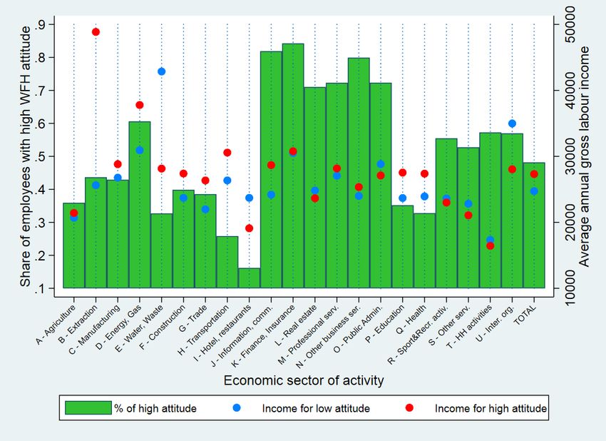
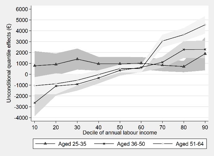
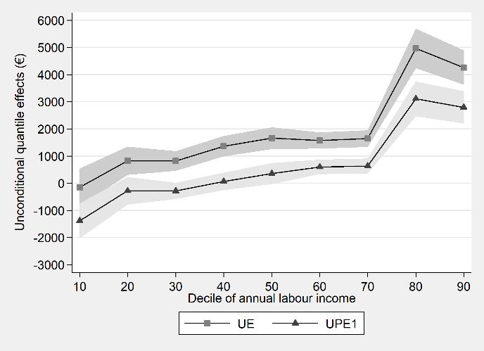
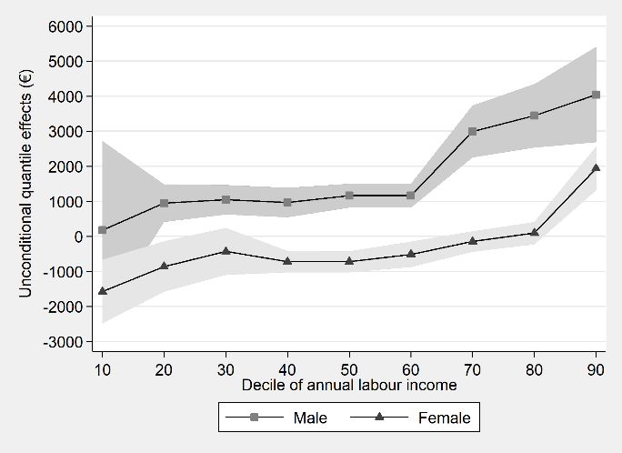
All that glitters is not gold. Influence of working from home on income inequality at the time of Covid-19 13

4.3 Influences of occupations attitude towards working from home
Table 3 highlights that the WFH attitude significantly affects the labour income distribution and
inequality. Specifically, RIF regression results suggest that replacing all employees having low WFH
attitude level with those having high attitude levels would determine an increase of both the mean
labour income up to €2,600 (we refer to that as ‘premium’) and the Gini index for about 0.04 points.
Considering that the mean labour income in our sample is equal to about €26,000 (see table 1), this
means that an overall positive variation of WFH attitude would lead to a 10% increase on the mean
labour income.

Table 3. Unconditional effects of WFH attitude on the mean and Gini index
 Mean value Gini index
 Group of employees
 UE UPE1 UPE2 UE UPE1 UPE2
 Total sample 2,589*** 1,291** 980 0.036** 0.044*** 0.035**
 Male 4,730*** 2,678** 2,338** 0.036 0.032 0.041
 Female 1,110** -75 -337 0.024** 0.031*** 0.008
 Aged 25-35 3,757*** 2,900** 2,706* 0.045 0.061 0.077*
 Aged 36-50 241 -238 -826 0.007 0.025 0.011
 Aged 51-64 4,964*** 2,613*** 2,508** 0.068*** 0.070*** 0.050*
 Less Covid-19 infected area 1,934* 777 465 0.026 0.050** 0.035
 More Covid-19 infected area 3,304*** 1,834** 1,372** 0.045* 0.039** 0.031*
Note: Standard errors are clustered by NUTS-3 region; *** p

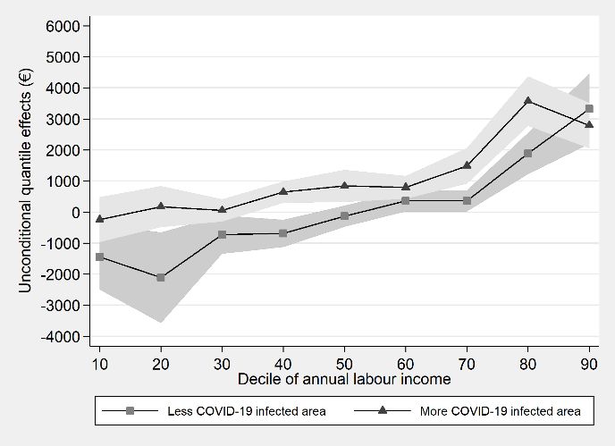
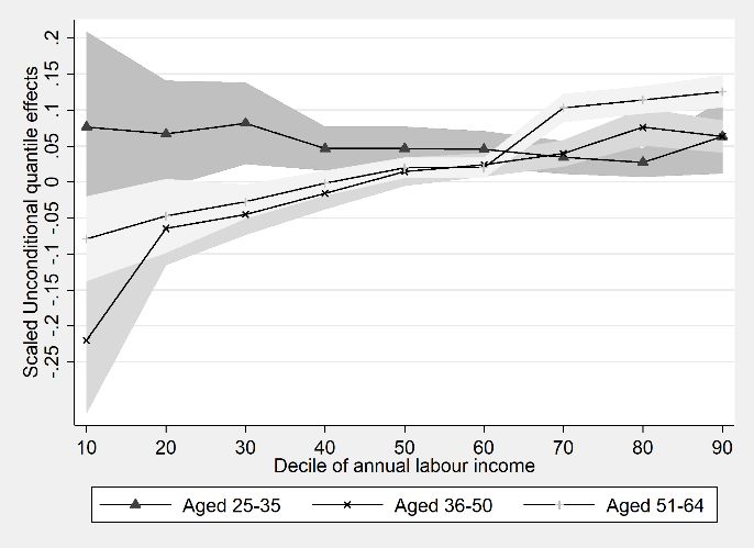
14 All that glitters is not gold. Influence of working from home on income inequality at the time of Covid-19

(2011) and Mussida and Picchio (2014) who find a glass ceiling effect in the gender wage gap in Italy6.
A positive change in WFH attitude levels among employees aged 25-35 would have a stable and
positive effect along their whole distribution (bottom-left panel of figure 4). At the opposite,
decreasing the number of employees with low WFH attitude levels would determine unequal
influences along labour income distribution of older employees. In particular, employees aged 51 or
more would report a wage penalty in the first three deciles and a relevant premium from the seventh
decile onwards (significantly higher than the other groups).
Finally, bottom-right panel of figure 4 shows that employees in more Covid-19 infected area would
benefit more from the overall WFH attitude improvement of occupations. This is an interesting and
important evidence as these territories actually need for this kind of policy, but its influence is still
unequal along the labour income distribution of their employees as it would be more in favor of high-
paid ones.

Figure 4. Unconditional effects of WFH attitude along the labour income distribution

Note: standard errors are clustered by NUTS-3 region. Shadowed area report confidence intervals at 90% level. Estimates by employees’
characteristics refer to the UPE1 specification. Estimates based on UPE2 specification are provided in figure A2. Complete estimates for the
pooled sample are provided in tables A4-A6.
Source: elaborations of the Authors on ICP 2013 and Inapp PLUS 2018 data

6
 Similarly Biagetti and Scicchitano (2014) report a larger male-female wage gap among high paid jobs in Italy.
The glass ceiling effect has been found also in Spain (Scicchitano 2014), in Sweden (Albrecht et al. 2003), in the
UK (Scicchitano 2012).

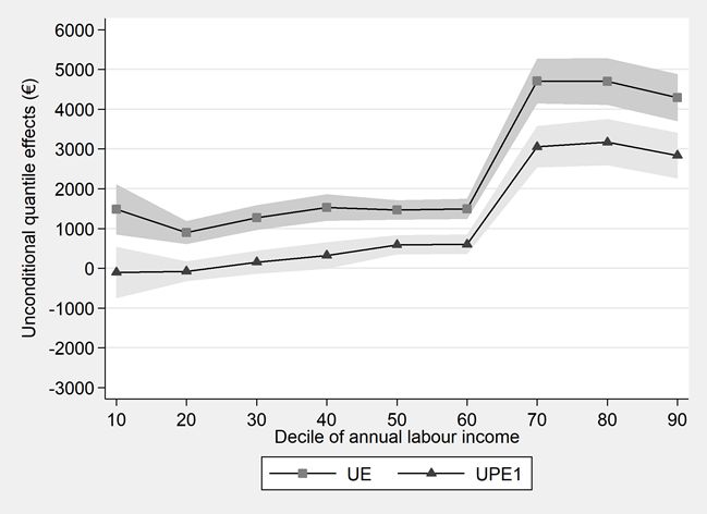
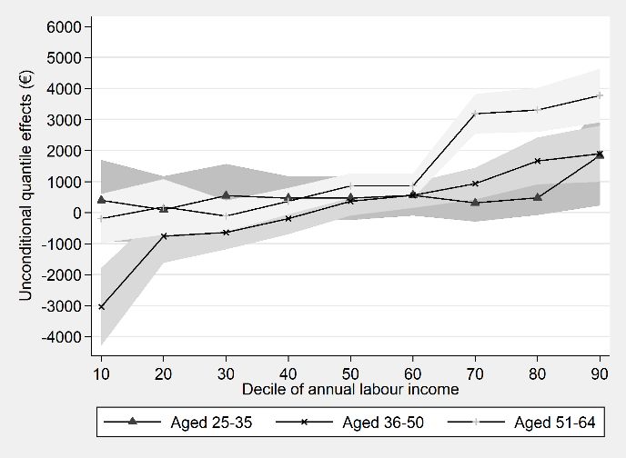
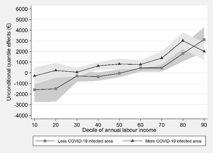
All that glitters is not gold. Influence of working from home on income inequality at the time of Covid-19 15

5. Robustness checks

In this section, we briefly summarize several robustness checks of the main results presented in the
paper, concerning scaled RIF regression results to point estimates, selection issue, exclusion of part-
time and temporary employees, different income inequality indexes, or including additional covariates
in the regressions.
First, as each group of employees reports on average different income levels with respect to the others
(see, for instance, wage gaps between male and female employees in table 1), we decided to also
present scaled UE and UPE estimates representing main results of our analysis. To obtain scaled
estimates, we divided recentered influence functions used as dependent variables by respective point
estimates (i.e. mean or quantile value of annual gross labour income of that specific group of
employees). Scaled estimates may be therefore interpreted as growth rates of the mean and decile
values related to marginal changes in the number of employees having a high WFH attitude level.
Scaled UE and UPE estimates presented in table 4 and figure 5 overall confirm the robustness of our
results.

Table 4. Scaled unconditional effects of WFH attitude on the mean
 Mean value
 Group of employees
 UE UPE1 UPE2
 Total employees 0.100*** 0.050** 0.038
 Male 0.161*** 0.091** 0.080**
 Female 0.050** -0.003 -0.015
 Aged 25-35 0.171*** 0.132** 0.123*
 Aged 36-50 0.009 -0.009 -0.032
 Aged 51-64 0.176*** 0.093*** 0.089**
 Less Covid-19 infected area 0.075* 0.030 0.018
 More Covid-19 infected area 0.125*** 0.070** 0.052**
Notes: standard errors are clustered by NUTS-3 region; *** p

16 All that glitters is not gold. Influence of working from home on income inequality at the time of Covid-19

Figure 5. Scaled unconditional effects of WFH attitude along the labour income distribution

Notes: standard errors are clustered by NUTS-3 region. Shadowed area report confidence intervals at 90% level. Estimates by employees’
characteristics refer to the UPE1 specification.
Source: elaborations of the Authors on ICP 2013 and Inapp PLUS 2018 data

In this robustness check, we adopt the two sets of covariates defined in section 3, thus UPE 1 (only
exogenous variables) and UPE 2 (including potentially endogenous variables on the actual job). We
believe that these sets of covariates considerably reduce the role of unobserved heterogeneity
between the two groups of workers. Nonetheless, even though controlling for a large number of
relevant characteristics that may affect both outcome and treatment selection, we cannot avoid that
other unobservable confounding factors may be still in place. Table A7 reports estimated coefficients
on the mean and nine decile values from the IPW approach. The effect of having a high WFH attitude
on the mean is equal to +3.9% controlling for UPE 1 variables and +3.5% when the UPE 2 set of
covariates is considered. Results indicate that the estimated influence of the WFH attitude on income
distribution is not substantially distorted by a selection bias, thus strengthening the evidence obtained
through the RIF method. Third, as our analysis is based on a definition of labour income which is annual
referred, we want to verify that our results are biased by the presence of part-time and temporary
employees in the sample. So, in this robustness check, we drop from the sample all employees having
these employment contracts. Results by including only full-time open-ended employees are presented
in table A8 and figure A3 and strongly corroborate our main conclusions.
Fourth, we run RIF estimates on two different income inequality indexes with respect to the one we
adopted (i.e. the Gini index): the mean log deviation and the Atkinson index with e=1. Results of these

All that glitters is not gold. Influence of working from home on income inequality at the time of Covid-19 17

tests, presented in table A9 for each group of employees and in table A10 for the pooled sample,
overall confirm the robustness of our main conclusions. Finally, we further enlarge the set of
covariates used for UPE estimates including other three probably endogenous variables. Specifically,
we include the physical proximity and the disease exposure indexes recently provided by Barbieri et
al. (2020) and the occupation skill level of employees to control for skill heterogeneity as suggested
by Picchio and Mussida (2011) and Leonida et al. (2020). As for the physical proximity index, it ranges
from 0 to 100 and it is measured for each occupation at 5-digit ISCO classification level through the
following question from the ICP 2013 survey: “During your work are you physically close to other
people?”. As for the disease exposure index, it ranges from 0 to 100 and it is measured for each
occupation at 5-digit ISCO classification level through the following question from the ICP 2013 survey:
“How often does your job expose you to diseases and infections?”. As for the occupation skill level, it
is included through a set of dummy variables representing different levels of the ISCO classification of
occupations. In particular, we define as: ‘Medium skill level’, employees in the fourth ISCO level (i.e.
clerical support workers); ‘High skill level’, employees in the third one (i.e. technicians and associate
professionals); ‘Very high skill level’, employees in the first two ISCO levels (i.e. managers and
professionals). The reference category is ‘Low skill level’. We label estimates based on this model
specification as UPE3 and we present them for the total sample in tables A.11 and A.12 in the appendix
in comparison with UPE2 ones. Outcomes of these robustness checks overall confirm that our main
results hold even considering these additional relevant covariates.

6. Conclusions

Based on a unique dataset and unconditional quantile regression methods, our analysis aims to
provide useful insights to policymakers who are designing strategies to adopt in the labour market for
future phases of the Covid-19 pandemic, as it might be longer than expected.
Although working from home (WFH) can represent the right answer to contain the infection spread,
potential ‘collateral effects’ of this working procedure on income inequality among employees should
not be underestimated. Our results show that increasing WFH attitude levels of occupations would
lead on average to a growth of labour income levels, probably because of their higher productivity.
However, it would also determine a rise of labour income inequality among Italian employees as
benefits from a positive change in occupations WFH attitude tend to be greater for male, older and
high-paid employees, as well as those living in provinces more affected by the novel coronavirus. Our
results hold after a number of robustness checks, regarding different income inequality indexes,
several model specifications, and scaled RIF regressions. Whether WFH is confirmed as a lasting
solution after the Covid-19 pandemic, our results suggest that it risks to exacerbate pre-existing
inequalities in the Italian labour market. In this respect, policies aimed at alleviating inequality7, like
income support measures broad enough to cover most vulnerable employees or training courses filling
potential knowledge gaps seem to be of outmost importance.

7
 Lucchese and Pianta (2020) look at the universal public health as a crucial element of an egalitarian policy.

18 All that glitters is not gold. Influence of working from home on income inequality at the time of Covid-19

Appendix

A. Descriptive statistics and additional estimates

Table A1. Variables description
Variable Description
 Continuous variable representing the annual gross labour income. All recentered influence functions on
Annual gross labour income
 distributional statistics are based on this variable.
 Binary variable reporting the level of WFH attitude. The WFH attitude is measured, for each occupation at
 5-digit ISCO classification level, through a composite index recently introduced by Barbieri et al. (2020).
 This index relies on replies to seven questions in the ICP 2013 survey questionnaire regarding: (i) the
 importance of performing general physical activities (which enters reversely); (ii) the importance of
 working with computers; (iii) the importance of manoeuvring vehicles, mechanical vehicles or equipment
High working from home
 (reversely); (iv) the requirement of face-to-face interactions (reversely); (v) the dealing with external
(WFH) attitude
 customers or with the public (reversely); (vi) the physical proximity (reversely); and (vii) the time spent
 standing (reversely). The WFH attitude is calculated as average of the listed seven items and ranges from
 0 to 100.
 Binary variable is equal to 1 for those having an index value over the sample mean (i.e. 52.2), and 0
 otherwise.
Female Binary variable taking value 1 for female, 0 for male.
Aged 36-50
 Binary variables representing the age group of individuals. The reference category is Aged 25-35.
Aged 51-64
Upper secondary education Binary variables representing the highest education level achieved. The reference category is composed
Tertiary education by Lower secondary education (or lower education level).
 Binary variables representing the migration status. An individual is 'Migrant within macro-region' if her
Migrant within macro-region region of birth and her region of residence belong to the same macro-region (i.e. North, Center, or South).
Migrant within country An individual is 'Migrant within country' if her region of birth belongs to a different macro-region with
Foreign migrant respect to her region of residence. An individual is 'Foreign migrant' if she moves from outside Italy. The
 reference category is Local.
Married Binary variable taking value 1 for married people, and 0 otherwise.
Household size = 2
Household size = 3 Binary variables representing the household size. The reference category is Single person (or Household
Household size = 4 size = 1).
Household size = 5 or more
 Binary variable taking value 1 for people living in households with at least one minor child, and 0
Presence of minors
 otherwise.
Small municipality Binary variables representing the size of the municipality of residence. Small municipality has a number of
Medium municipality inhabitants between 5,000 and 20,000, Medium municipality has 20,000 - 50,000 inhabitants, Big
Big municipality municipality counts 50,000 - 250,000 inhabitants, and Metropolitan city has 250,000 or more inhabitants.
Metropolitan city The reference category is Very small municipality (number of inhabitants lower than 5,000).
Centre
 Binary variables representing the macro-region of residence. The reference category is North.
South
Part-time open-ended
worker Binary variables representing the type of job contract. The reference category is Full-time open-ended
 worker.
Temporary worker and other
Public servant Binary variable taking value 1 for employees working in the public sector, and 0 otherwise.
 Variable representing the degree of Covid-19 infection at provincial level. The infection degree is
 measured as the incidence of Covid-19 cases on total population at provincial level. People live in a 'more
Less Covid-19 infected area Covid-19 infected' area if their province of residence reports an infection incidence over the sample
More Covid-19 infected area median (i.e. 3.2‰). Alternatively, they live in a 'less Covid-19 infected' area. Data on the overall Covid-19
 cases at provincial level are provided by the Italian Civil Protection Department (2020) and refers to the
 period between February 24 and May 5, 2020.

All that glitters is not gold. Influence of working from home on income inequality at the time of Covid-19 19

Table A2. Sample composition, mean and Gini index of annual labour income, mean value of the WFH
 attitude index and share of employees with high attitude level by economic sector of activity

 Sample composition Annual labour income WFH attitude

 % of
 Economic sector of activity employees
 Mean Std. Dev. Mean Gini index Mean
 with high
 attitude
 A - Agriculture 0.024 0.153 20,960 0.270 49.8 35.9
 B - Extraction 0.006 0.077 35,770 0.380 54.3 43.7
 C - Manufacturing 0.168 0.374 27,650 0.252 52.4 42.9
 D - Energy, Gas 0.016 0.127 35,084 0.356 56.5 60.6
 E - Water, Waste 0.005 0.068 38,049 0.424 51.0 32.7
 F - Construction 0.029 0.167 25,176 0.242 49.6 39.8
 G - Trade 0.098 0.298 23,662 0.305 48.4 38.6
 H - Transportation 0.049 0.216 27,445 0.262 49.6 25.8
 I - Hotel, restaurants 0.035 0.184 22,965 0.366 39.0 16.2
 J - Information, comm. 0.040 0.196 27,866 0.275 63.8 81.9
 K - Finance, Insurance 0.038 0.191 30,730 0.277 64.6 84.2
 L - Real estate 0.003 0.053 23,995 0.236 58.2 71.0
 M - Professional services 0.062 0.241 27,863 0.341 59.9 72.3
 N - Other business services 0.040 0.196 25,076 0.222 62.6 79.9
 O - Public Administration 0.070 0.254 27,581 0.254 59.8 72.3
 P - Education 0.124 0.329 25,040 0.194 47.9 35.2
 Q - Health 0.105 0.307 25,060 0.281 44.6 32.8
 R - Sport, recreational activ. 0.012 0.109 23,277 0.302 52.6 55.5
 S - Other services 0.068 0.252 21,895 0.316 53.3 52.7
 T - Household Activities 0.008 0.087 16,822 0.232 53.6 57.3
 U - International
 0.002 0.046 31,033 0.339 58.9 57.0
 organizations
 Total sample - - 25,979 0.280 52.4 48.2
Note: all descriptive statistics are computed with individual sample weights. Employees with high WFH attitude level are defined as those
reporting a value of the WFH attitude index over the sample median (i.e. 52.2).
Source: elaborations of the Authors on ICP 2013 and Inapp PLUS 2018 data

20 All that glitters is not gold. Influence of working from home on income inequality at the time of Covid-19

Table A3. Unconditional effects on the mean and Gini index in the total sample
 Mean value Gini index
 Variable
 UE UPE1 UPE2 UE UPE1 UPE2
 High WFH attitude 2,589*** 1,291** 980 0.036** 0.044*** 0.035**
 Female -8,870*** -6,090*** -0.022 -0.047***
 Aged 36-50 4,150*** 3,506*** 0.010 0.039**
 Aged 51-64 5,985*** 5,083*** -0.005 0.048*
 Upper secondary education 3,843*** 3,697*** -0.033 -0.010
 Tertiary education 9,938*** 9,671*** -0.009 0.054**
 Migrant within macro-region 1,331 2,158 0.091 0.077
 Migrant within country 18 -108 0.006 0.014
 Foreign migrant -761 -613 0.063** 0.049
 Married 3,486*** 2,908*** 0.034 0.046*
 Household size = 2 -1,652 -1,022 0.001 -0.008
 Household size = 3 -3,035*** -1,982* -0.016 -0.030
 Household size = 4 -1,845* -757 0.014 -0.004
 Household size = 5 or more -1,089 484 0.055 0.036
 Presence of minors -418 -636 -0.042 -0.045
 Small municipality 812 841 0.013 0.014
 Medium municipality -371 -465 -0.004 -0.006
 Big municipality 56 275 0.024 0.020
 Metropolitan city -596 -224 0.001 -0.003
 Center -2,172*** -1,863*** 0.003 -0.001
 South -2,432*** -1,541* 0.047** 0.053**
 Part-time open-ended worker -8,381*** 0.139***
 Temporary worker and other -6,504*** 0.095***
 Public servant 127 -0.053**
 Constant 24,731*** 22,431*** 20,808*** 0.263*** 0.248*** 0.173***
 Activity sector dummies No No Yes No No Yes
 Observations 14,307 14,307 14,307 14,307 14,307 14,307
 R-squared 0.002 0.043 0.061 0.001 0.004 0.016
Note: Notes: Standard errors are clustered by NUTS-3 region; *** p

All that glitters is not gold. Influence of working from home on income inequality at the time of Covid-19 21

Table A4. Unconditional effects of WFH attitude along the wage distribution (UE estimates)
 Variable p10 p20 p30 p40 p50 p60 p70 p80 p90
 High WFH attitude -153 828*** 820*** 1,363*** 1,660*** 1,571*** 1,645*** 4,965*** 4,261***
 Constant 11,772*** 15,638*** 18,780*** 20,244*** 21,904*** 23,534*** 26,164*** 26,664*** 32,323***
 Activity sector dummies No No No No No No No No No
 Observations 14,307 14,307 14,307 14,307 14,307 14,307 14,307 14,307 14,307
 R-squared 0.000 0.001 0.002 0.004 0.006 0.010 0.010 0.017 0.014
Note: Standard errors are clustered by NUTS-3 region; *** p

22 All that glitters is not gold. Influence of working from home on income inequality at the time of Covid-19

Table A6. Unconditional effects of WFH attitude along the wage distribution (UPE2 estimates)
 Variable p10 p20 p30 p40 p50 p60 p70 p80 p90
 High WFH attitude -1,554*** -85 -132 199 406* 652*** 677*** 2,829*** 2,333***
 Female -2,546*** -3,132*** -3,310*** -3,988*** -4,395*** -2,877*** -3,023*** -7,288*** -5,122***
 Aged 36-50 564 1,492*** 1,876*** 2,048*** 2,489*** 2,032*** 2,086*** 4,341*** 2,931***
 Aged 51-64 939 2,675*** 2,681*** 3,207*** 3,952*** 3,343*** 3,479*** 7,359*** 5,160***
 Upper secondary education 2,936*** 2,461*** 2,632*** 2,973*** 3,127*** 2,717*** 2,833*** 5,264*** 3,969***
 Tertiary education 4,649*** 4,704*** 5,325*** 6,517*** 7,075*** 5,517*** 5,776*** 13,002*** 10,937***
 Migrant within macro-region -2,877** -245 842* 1,551** 1,148* 456 278 1,193 1,476
 Migrant within country -865 -954** -21 -96 -71 119 134 667 -711
 Foreign migrant -2,604 -4,499*** -1,686** -1,147 -1,223 -474 -445 59 498
 Married 1,093** 404 543** 786*** 1,054*** 1,031*** 1,145*** 3,079*** 2,326***
 Household size = 2 -1,262* -60 -174 -163 -564 -503 -616* -471 -309
 Household size = 3 -940 -333 -494 -458 -950** -877*** -1,017*** -1,421* -444
 Household size = 4 -1,061 -280 -291 -295 -466 -461 -546 0 372
 Household size = 5 or more -1,281 -614 -150 7 -132 232 152 1,467 1,512
 Presence of minors 461 1,086*** 690** 982*** 801*** 490** 605*** 523 223
 Small municipality 382 100 495* 42 -46 -83 -10 -461 -281
 Medium municipality -299 -119 267 26 -24 -195 -223 -981* -624
 Big municipality -698 -306 228 -160 38 -226 -159 -710 18
 Metropolitan city -466 -432 329 410 567 44 107 655 936**
 Center -1,235*** -1,743*** -1,142*** -1,052*** -1,069*** -794*** -794*** -2,152*** -1,254***
 South -4,460*** -3,131*** -1,597*** -1,529*** -1,444*** -857*** -862*** -1,579*** -1,011**
 Part-time open-ended worker -10,851*** -15,408*** -9,378*** -8,713*** -7,709*** -4,231*** -4,370*** -6,760*** -3,217***
 Temporary worker and other -9,793*** -9,129*** -5,859*** -6,051*** -5,609*** -2,927*** -3,020*** -4,330*** -2,028***
 Public servant 2,340*** 2,090*** 1,427*** 1,342*** 993*** 225 195 -1,042* -1,041**
 Constant 14,033*** 14,773*** 17,243*** 18,712*** 20,447*** 21,545*** 24,139*** 21,468*** 28,488***
 Activity sector dummies Yes Yes Yes Yes Yes Yes Yes Yes Yes
 Observations 14,307 14,307 14,307 14,307 14,307 14,307 14,307 14,307 14,307
 R-squared 0.161 0.344 0.322 0.289 0.248 0.208 0.206 0.170 0.101
Note: standard errors are clustered by NUTS-3 region; *** p

All that glitters is not gold. Influence of working from home on income inequality at the time of Covid-19 23

Table A7. Estimated effect of high WFH attitude on the mean and along the labour income distribution (IPW estimation method)

 Model
 High WFH attitude Mean value p10 p20 p30 p40 p50 p60 p70 p80 p90
 spec.
 Male 0.082*** 0.000 0.083*** 0.077*** 0.035 0.067*** 0.107*** 0.078*** 0.057** 0.134***
 Female -0.009 -0.074** 0.000 0.000 0.000 0.000 0.000 0.000 0.036*** 0.065***
 Aged 25-35 0.018 0.000 0.046 0.100*** 0.000 0.000 0.000 0.000 0.067*** 0.013
 UPE 1

 Aged 36-50 0.019 -0.065*** 0.000 0.000 0.000 0.000 0.000 0.067*** 0.069*** 0.112***
 Aged 51-64 0.068*** -0.111*** 0.000 0.038*** 0.000 0.067*** 0.072*** 0.102*** 0.126*** 0.303***
 Less Covid-19 infected area 0.021 -0.069** 0.000 0.000 0.000 0.000 0.000 0.072*** 0.069*** 0.112***
 More Covid-19 infected area 0.059*** 0.000 0.000 0.042*** 0.077*** 0.071*** 0.034*** 0.072*** 0.171*** 0.212***
 Male 0.070*** 0.000 0.083*** 0.038** 0.000 0.067*** 0.107*** 0.065*** 0.057*** 0.134***
 Female 0.006 0.000 0.012 0.100*** 0.000 0.000 0.000 0.000 0.000 0.000
 Aged 25-35 -0.011 -0.064 0.000 0.000 0.000 0.000 0.000 0.000 0.033 0.000
 UPE 2

 Aged 36-50 0.011 -0.065* 0.000 0.000 0.000 0.000 0.000 0.000 0.021 0.112***
 Aged 51-64 0.076*** -0.029 0.000 0.077*** 0.071*** 0.067*** 0.072*** 0.102*** 0.061* 0.191**
 Less Covid-19 infected area 0.035 -0.015 0.000 0.000 0.000 0.000 0.000 0.072*** 0.000 0.112***
 More Covid-19 infected area 0.041** 0.000 0.000 0.042** 0.077*** 0.042*** 0.040*** 0.072*** 0.114*** 0.212***
Note: standard errors are clustered by NUTS-3 region; *** p

24 All that glitters is not gold. Influence of working from home on income inequality at the time of Covid-19

Table A8. Unconditional effects of WFH attitude on the mean and Gini index considering only full-time
 open-ended employees

 Mean value Gini index
 Group of employees
 UE UPE1 UPE2 UE UPE1 UPE2
 Total sample 3,904*** 2,476*** 2,092** 0.043* 0.047** 0.035
 Male 5,449*** 3,305** 3,297** 0.046 0.039 0.039
 Female 1,934*** 940*** 369 0.031** 0.034*** 0.009
 Aged 25-35 3,757*** 2,900** 2,706* 0.045 0.061 0.077*
 Aged 36-50 241 -238 -826 0.007 0.025 0.011
 Aged 51-64 4,964*** 2,613*** 2,508** 0.068*** 0.070*** 0.050*
 Less Covid-19 infected area 0.005 0.011 0.028 -0.017 -0.008 0.007
 More Covid-19 infected area 6,031*** 3,868*** 3,417** 0.079*** 0.075*** 0.059*
Note: standard errors are clustered by NUTS-3 region; *** p

All that glitters is not gold. Influence of working from home on income inequality at the time of Covid-19 25

Table A10. Unconditional effects on the mean log deviation and Atkinson index (e=1) in the total sample
 Mean log deviation Atkinson index (e=1)
 Variable
 UE UPE1 UPE2 UE UPE1 UPE2
 High WFH attitude 0.030 0.045** 0.038* 0.025 0.037** 0.032*
 Female -0.026 -0.043* -0.021 -0.036*
 Aged 36-50 0.011 0.041* 0.009 0.034*
 Aged 51-64 -0.006 0.048 -0.005 0.040
 Upper secondary education -0.050* -0.027 -0.042* -0.023
 Tertiary education -0.035 0.024 -0.030 0.020
 Migrant within macro-region 0.114* 0.101* 0.095* 0.084*
 Migrant within country 0.011 0.020 0.009 0.016
 Foreign migrant 0.040 0.028 0.034 0.024
 Married 0.030 0.043 0.025 0.035
 Household size = 2 0.001 -0.008 0.000 -0.007
 Household size = 3 -0.026 -0.040 -0.022 -0.034
 Household size = 4 0.009 -0.008 0.007 -0.007
 Household size = 5 or more 0.064 0.045 0.053 0.037
 Presence of minors -0.046 -0.049 -0.039 -0.041
 Small municipality 0.013 0.015 0.011 0.012
 Medium municipality 0.001 -0.001 0.001 -0.001
 Big municipality 0.037 0.034 0.031 0.029
 Metropolitan city 0.002 -0.002 0.002 -0.002
 Center 0.003 -0.002 0.003 -0.001
 South 0.059** 0.063** 0.049** 0.053**
 Part-time open-ended worker 0.114*** 0.095***
 Temporary worker and other 0.102*** 0.085***
 Public servant -0.063*** -0.052***
 Constant 0.167*** 0.167*** 0.075 0.154*** 0.154*** 0.077*
 Activity sector dummies No No Yes No No Yes
 Observations 14,307 14,307 14,307 14307 14307 14307
 R-squared 0.000 0.004 0.012 0.000 0.004 0.012
Note: standard errors are clustered by NUTS-3 region; *** p

26 All that glitters is not gold. Influence of working from home on income inequality at the time of Covid-19

Table A11. Unconditional effects on the mean and inequality indicators in the total sample (UPE2 and UPE3 estimates)
 Mean value Gini index Mean log deviation Atkinson index (e=1)
 Variable
 UPE2 UPE3 UPE2 UPE3 UPE2 UPE3 UPE2 UPE3
 High SW attitude 980 183 0.035** 0.046* 0.038* 0.056* 0.032* 0.047*
 Female -6,090*** -5,908*** -0.047*** -0.041** -0.043* -0.037 -0.036* -0.031
 Aged 36-50 3,506*** 3,442*** 0.039** 0.036** 0.041* 0.038* 0.034* 0.032*
 Aged 51-64 5,083*** 4,913*** 0.048* 0.044* 0.048 0.045 0.040 0.037
 Upper secondary education 3,697*** 2,850*** -0.010 -0.000 -0.027 -0.011 -0.023 -0.009
 Tertiary education 9,671*** 6,783*** 0.054** 0.036* 0.024 0.016 0.020 0.014
 Migrant within macro-region 2,158 1,938 0.077 0.072 0.101* 0.096 0.084* 0.080
 Migrant within country -108 -311 0.014 0.009 0.020 0.015 0.016 0.012
 Foreign migrant -613 -257 0.049 0.045 0.028 0.023 0.024 0.019
 Married 2,908*** 2,772*** 0.046* 0.046* 0.043 0.042 0.035 0.035
 Household size = 2 -1,022 -906 -0.008 -0.006 -0.008 -0.007 -0.007 -0.006
 Household size = 3 -1,982* -1,916* -0.030 -0.029 -0.040 -0.039 -0.034 -0.032
 Household size = 4 -757 -682 -0.004 -0.003 -0.008 -0.008 -0.007 -0.006
 Household size = 5 or more 484 438 0.036 0.037 0.045 0.046 0.037 0.038
 Presence of minors -636 -642 -0.045 -0.045 -0.049 -0.049 -0.041 -0.041
 Small municipality 841 900 0.014 0.016 0.015 0.016 0.012 0.014
 Medium municipality -465 -471 -0.006 -0.004 -0.001 0.001 -0.001 0.001
 Big municipality 275 319 0.020 0.022 0.034 0.036 0.029 0.030
 Metropolitan city -224 -305 -0.003 -0.002 -0.002 0.000 -0.002 0.000
 Center -1,863*** -1,747*** -0.001 -0.002 -0.002 -0.003 -0.001 -0.003
 South -1,541* -1,541* 0.053** 0.050** 0.063** 0.060** 0.053** 0.050**
 Part-time open-ended worker -8,381*** -7,805*** 0.139*** 0.146*** 0.114*** 0.120*** 0.095*** 0.100***
 Temporary worker and other -6,504*** -6,279*** 0.095*** 0.095*** 0.102*** 0.101*** 0.085*** 0.084***
 Public servant 127 -644 -0.053** -0.061*** -0.063*** -0.069*** -0.052*** -0.058***
 Physical proximity index -33 -0.001 -0.001* -0.001*
 Diseases exposure index 39** 0.001** 0.001** 0.001**
 Average skill level 497 -0.067*** -0.092*** -0.077***
 High skill level 2,094** -0.042* -0.052* -0.043*
 Very high skill level 6,849*** 0.054* 0.031 0.026
 Constant 20,808*** 21,895*** 0.173*** 0.207*** 0.075 0.115 0.077* 0.110*
 Activity sector dummies Yes Yes Yes Yes Yes Yes Yes Yes
 Observations 14,307 14,307 14,307 14,307 14,307 14,307 14,307 14,307
 R-squared 0.061 0.062 0.016 0.019 0.012 0.014 0.012 0.014
Note: standard errors are clustered by NUTS-3 region; *** p