Ambient air quality in the Kathmandu Valley, Nepal, during the pre-monsoon: concentrations and sources of particulate matter and trace gases
←
→
Page content transcription
If your browser does not render page correctly, please read the page content below
Atmos. Chem. Phys., 20, 2927–2951, 2020
https://doi.org/10.5194/acp-20-2927-2020
© Author(s) 2020. This work is distributed under
the Creative Commons Attribution 4.0 License.

Ambient air quality in the Kathmandu Valley, Nepal, during
the pre-monsoon: concentrations and sources of particulate
matter and trace gases
Md. Robiul Islam1 , Thilina Jayarathne1 , Isobel J. Simpson2 , Benjamin Werden3 , John Maben4 , Ashley Gilbert1 ,
Puppala S. Praveen5 , Sagar Adhikari5,6 , Arnico K. Panday5 , Maheswar Rupakheti7 , Donald R. Blake2 ,
Robert J. Yokelson8 , Peter F. DeCarlo3,9 , William C. Keene4 , and Elizabeth A. Stone1,10
1 Department    of Chemistry, University of Iowa, Iowa City, IA, USA
2 Department    of Chemistry, University of California-Irvine, Irvine, CA, USA
3 Department of Civil, Architectural, and Environmental Engineering, Drexel University, Philadelphia, PA, USA
4 Department of Environmental Sciences, University of Virginia, Charlottesville, VA, USA
5 International Centre for Integrated Mountain Development (ICIMOD), Lalitpur, Nepal
6 MinErgy Pvt. Ltd, Lalitpur, Nepal
7 Institute for Advanced Sustainability Studies, Potsdam, Germany
8 Department of Chemistry, University of Montana, Missoula, MT, USA
9 Department of Environmental Health and Engineering, Johns Hopkins University, Baltimore, MD, USA
10 Department of Chemical and Biochemical Engineering, University of Iowa, Iowa City, IA, USA

Correspondence: Elizabeth A. Stone (betsy-stone@uiowa.edu)

Received: 5 April 2019 – Discussion started: 8 May 2019
Revised: 22 November 2019 – Accepted: 8 December 2019 – Published: 11 March 2020

Abstract. The Kathmandu Valley in Nepal is a bowl-shaped         monium (9 %), chloride (2 %), calcium (1 %), magnesium
urban basin that experiences severe air pollution that poses     (0.05 %), and potassium (1 %). Large diurnal variability in
health risks to its 3.5 million inhabitants. As part of the      temperature and relative humidity drove corresponding vari-
Nepal Ambient Monitoring and Source Testing Experiment           ability in aerosol liquid water content, the gas–aerosol phase
(NAMaSTE), ambient air quality in the Kathmandu Valley           partitioning of NH3 , HNO3 , and HCl, and aerosol solution
was investigated from 11 to 24 April 2015, during the pre-       pH. The observed levels of gas-phase halogens suggest that
monsoon season. Ambient concentrations of fine and coarse        multiphase halogen-radical chemistry involving both Cl and
particulate matter (PM2.5 and PM10 , respectively), online       Br impacted regional air quality. To gain insight into the ori-
PM1 , inorganic trace gases (NH3 , HNO3 , SO2 , and HCl),        gins of organic carbon (OC), molecular markers for primary
and carbon-containing gases (CO2 , CO, CH4 , and 93 non-         and secondary sources were quantified. Levoglucosan (av-
methane volatile organic compounds; NMVOCs) were quan-           eraging 1230 ± 1154 ng m−3 ), 1,3,5-triphenylbenzene (0.8 ±
tified at a semi-urban location near the center of the valley.   0.6 ng m−3 ), cholesterol (2.9±6.6 ng m−3 ), stigmastanol (1.0
Concentrations and ratios of NMVOC indicated origins pri-        ±0.8 ng m−3 ), and cis-pinonic acid (4.5 ± 1.9 ng m−3 ) in-
marily from poorly maintained vehicle emissions, biomass         dicate contributions from biomass burning, garbage burn-
burning, and solvent/gasoline evaporation. During those 2        ing, food cooking, cow dung burning, and monoterpene sec-
weeks, daily average PM2.5 concentrations ranged from 30 to      ondary organic aerosol, respectively. Drawing on source pro-
207 µg m−3 , which exceeded the World Health Organization        files developed in NAMaSTE, chemical mass balance (CMB)
24 h guideline by factors of 1.2 to 8.3. On average, the non-    source apportionment modeling was used to estimate contri-
water mass of PM2.5 was composed of organic matter (48 %),       butions to OC from major primary sources including garbage
elemental carbon (13 %), sulfate (16 %), nitrate (4 %), am-      burning (18 ± 5 %), biomass burning (17 ± 10 %) inclusive

Published by Copernicus Publications on behalf of the European Geosciences Union.
2928                                                      Md. R. Islam et al.: Ambient air quality in the Kathmandu Valley

of open burning and biomass-fueled cooking stoves, and            widespread and under-sampled combustion sources in Nepal.
internal-combustion (gasoline and diesel) engines (18±9 %).       Source characterization measurements included trace gases
Model sensitivity tests with newly developed source profiles      (Stockwell et al., 2016) and particulate matter (Goetz et al.,
indicated contributions from biomass burning within a fac-        2018; Jayarathne et al., 2018), as well as optical proper-
tor of 2 of previous estimates but greater contributions from     ties of aerosols (Stockwell et al., 2016). The characterized
garbage burning (up to three times), indicating large potential   sources included brick kilns, garbage burning, power genera-
impacts of garbage burning on regional air quality and the        tors, diesel groundwater pumps, idling motorcycles, cooking
need for further evaluation of this source. Contributions of      stoves, crop residue burning, and open burning of biofuels.
secondary organic carbon (SOC) to PM2.5 OC included those         As part of NAMaSTE, a regional monitoring station was also
originating from anthropogenic precursors such as naphtha-        installed to probe the relative contribution of these sources to
lene (10 ± 4 %) and methylnaphthalene (0.3 ± 0.1 %) and           ambient air quality. In addition, new emissions data are being
biogenic precursors for monoterpenes (0.13 ± 0.07 %) and          incorporated into regional air quality models for the region
sesquiterpenes (5 ± 2 %). An average of 25 % of the PM2.5         (Zhong et al., 2019).
OC was unapportioned, indicating the presence of additional          High daily average concentrations of PM2.5 (up to
sources (e.g., evaporative and/or industrial emissions such as    160 µg m−3 ) (Shakya et al., 2017a) and PM10 (up to
brick kilns, food cooking, and other types of SOC) and/or un-     579 µg m−3 ) have been documented in the Kathmandu Valley
derestimation of the contributions from the identified source     (Giri et al., 2006). A satellite-derived aerosol optical depth
types. The source apportionment results indicate that an-         study indicates substantial increases in particulate loading in
thropogenic combustion sources (including biomass burning,        the Kathmandu Valley and nearby background sites over the
garbage burning, and fossil fuel combustion) were the great-      past 15 years (Mahapatra et al., 2019). Measured components
est contributors to PM2.5 and, as such, should be considered      of regional PM have included black carbon (BC; 17 %), sul-
primary targets for controlling ambient PM pollution.             fate (17 %), and ammonium (11 %) in PM2.5 (Shakya et al.,
                                                                  2017a) and organic carbon (OC; 23 %) and nitrate (2.5 %)
                                                                  in PM10 (Kim et al., 2015). Carbon isotope analysis of bulk
                                                                  aerosol sampled during the winter of 2007–2008 in the Kath-
1   Introduction                                                  mandu Valley suggested that a major fraction of particulate
                                                                  OC originated from primary sources (69 %), particularly lo-
According to the World Health Organization (WHO, 2016),           cal fossil fuel emissions (39 %) (Shakya et al., 2010). A
4.2 million (or 7.6 % of all) premature deaths globally dur-      recent carbon isotope study observed that fossil fuel con-
ing 2016 were linked to ambient air pollution. The majority       tributed 67 % of the black carbon during April 2013 in the
of these premature deaths occurred in low- to middle-income       Kathmandu Valley (Li et al., 2016).
countries in the South Asia, East Asia, and western Pacific re-      An earlier chemical mass balance (CMB) source ap-
gions. The Kathmandu Valley in Nepal is home to more than         portionment study at Godawari, at the southeast edge of
3.5 million residents who suffer from high levels of air pollu-   the Kathmandu Valley identified sources of PM2.5 OC as
tants, including particulate matter (PM), ozone (O3 ), carbon     biomass burning (21 %), fossil fuel combustion (7 %), and
monoxide (CO), and volatile organic compounds (VOCs)              secondary organic aerosol (SOA) from biogenic precursors
(Bhardwaj et al., 2018; Kiros et al., 2016; Mahata et al.,        (3 %) (Stone et al., 2010). However, the relative contribu-
2018; Putero et al., 2015; Sarkar et al., 2016; Wan et al.,       tions of biomass and fossil fuel to elemental carbon (EC)
2019) that are expected to have severe health impacts (Gu-        were highly uncertain due to large variability in EC emis-
rung and Bell, 2013).                                             sions with respect to combustion efficiency and air-to-fuel
   Effective mitigation of air pollution requires understand-     ratios. A significant fraction of PM2.5 OC (54 %–84 %) in
ing the major contributing sources. PM emissions contain          that study was unapportioned suggesting significant contri-
molecular and elemental fingerprints that reflect the mate-       butions from other primary and secondary sources. Assess-
rial from which the PM was generated and the process(es) by       ments of PM sources in this region were challenging due
which it formed. For organic aerosol sources, these chemi-        in part to poorly characterized emissions from brick kilns,
cal fingerprints include molecular markers that are defined as    garbage burning, and local industries (Stone et al., 2010).
chemical species unique to a PM source category (Schauer          Anthropogenic SOA was also identified as a likely source
et al., 1996). Well-established molecular markers for pri-        of PM2.5 that was not previously apportioned (Stone et al.,
mary (direct emissions) and secondary (produced in the at-        2012).
mosphere from reactive precursors) sources are summarized            The primary goal of the study reported herein is to charac-
in Table 1. These species can be used to identify sources of      terize the composition of ambient gases and PM in the Kath-
PM in ambient air both directly and through source appor-         mandu Valley, Nepal, and apportion major sources based on
tionment modeling.                                                new knowledge of source-specific emissions within the re-
   The Nepal Ambient Monitoring and Source Testing Ex-            gion. Our specific objectives are to (1) quantify atmospheric
periment (NAMaSTE) was initiated in 2015 to characterize          loadings of volatile carbon-containing compounds (CO2 ,

Atmos. Chem. Phys., 20, 2927–2951, 2020                                            www.atmos-chem-phys.net/20/2927/2020/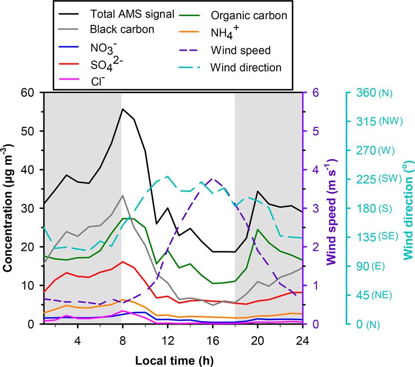
Md. R. Islam et al.: Ambient air quality in the Kathmandu Valley                                                               2929

Table 1. Molecular markers for primary or secondary sources of particulate matter.

                 Source                                Molecular marker                       Reference
                 Biomass burning                       Levoglucosan                           Simoneit et al. (1999)
                 Fossil fuel combustion/evaporation    Hopanes                                Schauer et al. (1999)
                 Food cooking                          Sterols                                Rogge et al. (1991)
                 Cow dung burning                      Stigmastanol                           Sheesley et al. (2003)
                 Garbage/plastic burning               1,3,5-Triphenylbenzene                 Simoneit et al. (2005)
                 Vegetative detritus                   n-Alkanes with odd carbon preference   Rogge et al. (1993)
                 Isoprene SOA                          Methyltetrols                          Kleindienst et al. (2007)
                 Monoterpene SOA                       cis-Pinonic acid                       Kleindienst et al. (2007)
                 Sesquiterpene SOA                     β-Caryophyllinic acid                  Jaoui et al. (2007)
                 Naphthalene SOA                       Phthalic acid                          Kleindienst et al. (2012)
                 2-Methylnaphthalene SOA               4-Methylphthalic acid                  Kleindienst et al. (2012)

CO, CH4 , and 93 non-methane volatile organic compounds;               averaged every 5 min. From 23 to 26 April, on-site meteoro-
NMVOCs), inorganic trace gases (NH3 , SO2 , HNO3 , HCl,                logical measurements were not available so meteorological
total volatile inorganic Br), and PM mass in the Kathmandu             conditions recorded at the Tribhuvan International Airport in
Valley during the pre-monsoon season; (2) chemically char-             Kathmandu, ca. 4 km to the west of Bode, were used instead.
acterize the major carbonaceous and ionic constituents of
PM; and (3) apportion organic carbon (OC) to its sources us-           2.2    PM and reactive trace gas sample collection
ing CMB modeling with region-specific source profiles when
available. This work is designed to contribute to advancing            A medium volume sampler (URG-3000 ABC) was placed on
the understanding of the role of combustion and other ma-              the rooftop of a five-story building at Bode, approximately
jor pollution sources in South Asia and their effects on air           15 m (50 ft) above the ground. PM samples were collected
quality.                                                               from 11 to 24 April 2015, during daytime (08:00 to 17:30)
                                                                       and nighttime (18:00 to 07:30) intervals. PM2.5 was sampled
                                                                       downstream of two 2.5 µm sharp-cut cyclones and PM10 was
2     Methods                                                          sampled downstream of a 10 µm sharp-cut impaction plate.
                                                                       Both air streams were split to collect four discrete PM sam-
2.1    Site description                                                ples in each size bin (total of eight samples per time inter-
                                                                       val), at nominal flow rates of 7.4 L min−1 each. The flow
Ambient air was sampled at Bode (27.689◦ N, 85.395◦ E;                 rate through each channel was measured before and after
1345 m a.s.l.), which is a semi-urban location close to the            the sample collection with a calibrated rotameter (Gilmont
geographic center of the Kathmandu Valley (Fig. S1 in                  Inst., Barrington, IL). PM in each size range was sampled on
the Supplement). Bode was the measurement supersite dur-               three 47 mm quartz fiber filters (QFFs; Tissuquartz, Pall Life
ing the Sustainable Atmosphere for the Kathmandu Valley-               Sciences, East Hills, New York) and one 47 mm Teflon fil-
Atmospheric Brown Clouds (SusKat-ABC) international air                ter (Teflo Membrane, 2.0 µm pore size, Pall Life Sciences).
pollution measurement campaign (Mahata et al., 2017, 2018;             QFFs were pre-cleaned by baking at 550 ◦ C for 18 h to re-
Sarkar et al., 2016). Bode is located in Madhyapur-Thimi               move organic species (Stone et al., 2007). Following collec-
Municipality and three major cities are located nearby: Kath-          tion, exposed PM samples were transferred to polystyrene
mandu Metropolitan City to the west, Lalitpur Metropoli-               petri dishes lined with pre-cleaned aluminum foil, capped,
tan City to the southwest, and Bhaktapur Municipality to the           sealed with Teflon tape, stored frozen in sealed polyethylene
southeast. The Bode supersite was located in a newly devel-            bags, and shipped to the University of Iowa for analysis.
oping suburban area that started with a grid of streets placed            Soluble reactive trace gases were sampled downstream of
across what were agricultural fields, with a gradual filling           two of the PM2.5 QFFs during daytime and nighttime pe-
in of houses on individual plots, while a lot of fields and            riods using a filter pack technique (Bardwell et al., 1990;
empty plots still remain. Nearby the Bode site are agricul-            Keene et al., 2009; Pszenny et al., 2004). Total volatile in-
tural fields, the Bhaktapur Industrial Estate with several small       organic NO3 and Cl (dominated by and hereafter referred to
pharmaceutical, plastic, and metal industries, and about 19            as HNO3 and HCl, respectively), SO2 , and total volatile in-
brick kilns located within 5 km to the east and southeast of           organic Br− (Brt ) were sampled using a three-stage, 47 mm,
the site. Meteorological conditions (temperature, relative hu-         Teflon filter pack housing configured with a QFF for PM col-
midity (RH), barometric pressure, global radiation and pre-            lection (as described above) followed by tandem rayon filters
cipitation) were measured at Bode for this study with data             (Schleicher and Schuell, 8S) impregnated with a solution of

www.atmos-chem-phys.net/20/2927/2020/                                                  Atmos. Chem. Phys., 20, 2927–2951, 2020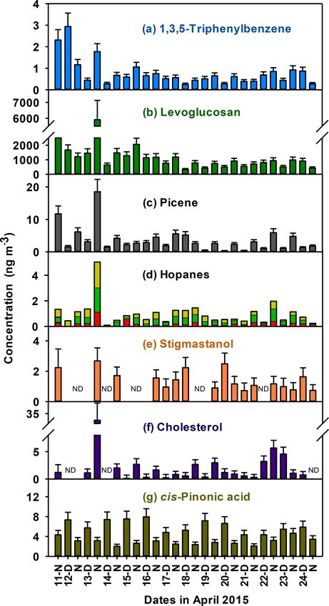
2930                                                     Md. R. Islam et al.: Ambient air quality in the Kathmandu Valley

10 % potassium carbonate (K2 CO3 ) and 10 % glycerol. NH3        ing an analytical microbalance (Mettler Toledo XP26). PM
was sampled in parallel using an otherwise identical filter      mass per filter was converted to mass concentration (µg m−3 )
pack configured with tandem rayon filters impregnated with       using sampled air volume after field blank subtraction. The
a solution of 10 % citric acid (C6 H8 O7 ) and 10 % glycerol.    analytical uncertainties in the mass measurements were cal-
   In total, 27 sets of ambient PM and reactive gas samples      culated following Jayarathne et al. (2018). The PM2.5 data
were collected. Field blanks were prepared every fifth sam-      for the nighttime periods of 12 and 13 April were excluded
pling period by loading, mounting, recovering, unloading,        due to sampling errors and filter damage, respectively.
and processing filter housings using otherwise identical pro-
cedures as those for samples but without pulling air through     2.5   Organic and elemental carbon measurement
them. All filter housings and samples were loaded and un-
loaded using clean-handling procedures. Impregnated filters      Organic carbon (OC) and elemental carbon (EC) were
were stored in polystyrene petri dishes that were capped,        measured following the National Institute for Occupational
sealed with Teflon tape, stored frozen in polyethylene bags,     Safety and Health (NIOSH) 5040 method (NIOSH, 2003) us-
and shipped to the University of Virginia for analysis.          ing 1.0 cm2 filter punches from sampled QFF (Sunset OC-EC
   Submicron PM (PM1 ) was characterized in parallel for         Aerosol Analyzer, Sunset Laboratories, Tigard, OR) (Birch
non-refractory constituents using a high-resolution aerosol      and Cary, 1996). OC data were field blank subtracted, while
mass spectrometer (HR-AMS) (DeCarlo et al., 2006). The           EC was not detected on field blanks. The uncertainties in OC
inlet for the AMS was located within 5 m of the URG sam-         and EC measurements were calculated following Jayarathne
pler. Samples were size selected through a PM2.5 cyclone,        et al. (2018).
and dried to below 30 % RH by a counterflow Nafion dryer.
                                                                 2.6   Analysis of particulate inorganic ions
The AMS measures mass and composition of non-refractory
PM1 at 1 min time resolution. Calibrations were undertaken       Water-soluble inorganic ions in PM were extracted in
for alignment, mass (ionization efficiency), and particle siz-   5 mL deionized water and analyzed by ion exchange chro-
ing. Frequent, intermittent power outages at Bode interrupted    matography (IC) with conductivity detection (Dionex-ICS
AMS operations necessitating long restart times and signifi-     5000), with details of the analytical method, uncertainties,
cant losses of sampling. Due to associated data losses, only     and detection limit calculations provided by Jayarathne et
10 of the filter samples aligned with concurrent AMS data        al. (2014). Unusually high concentrations of Na+ , Mg2+ ,
across the entire periods: 16 April nighttime to 17 April day-   Ca2+ , and F− were observed in the field blanks collected
time, 18 April daytime to 21 April daytime, and 22 April         on 15 April and PM samples collected from 15 to 17 April,
daytime. An in-depth analysis of the HR-AMS data will be         indicating likely contamination of these samples. Thus, con-
the subject of a forthcoming paper, but general observations     centrations of these ions during this time period were not re-
will be used here to provide a higher time resolution context    ported and were excluded in the calculation of average con-
for the filter measurements (see Sect. 3.2.1 for a discussion    centrations.
of PM mass and Sect. 3.2.3 for sulfate concentrations).
                                                                 2.7   Analysis of reactive trace gases
2.3    Whole-air samples
                                                                 Exposed rayon filters were extracted under sonication in
Whole-air samples (WASs) were collected from 16 to               5 mL of deionized water and analyzed by IC (Dionex-
24 April 2015 before 08:25 or after 18:00 and analyzed           ICS 3000, dual channel). The anion channel was configured
for CO2 , CO, CH4 , and 93 NMVOCs using multi-column             with Dionex guard (AG-4A 4 × 50 mm) and analytical (AS-
gas chromatography (Simpson et al., 2011; Stockwell et al.,      4A 4 × 250 mm) columns and a Dionex Anion Micro Mem-
2016). The WAS analytical details, including calibration pro-    brane Suppressor (AMMS). The cation channel was config-
cedures, are described in detail in Simpson et al. (2011).       ured with Dionex guard (IonPac CG16: 5 × 50 mm) and an-
While the WAS sampling was cut short by the Gorkha earth-        alytical (IonPac CG16: 5 × 250 mm) columns and a Thermo
quake on 25 April 2015 and only nine samples were col-           Scientific Dionex Cation Electrolytically Regenerated Sup-
lected, the limited WAS sampling still provides useful con-      pressor (CERS 500: 4 mm). Standard solutions were matrix
text for VOC levels and sources in the area.                     matched with sample extracts. Analytical results for sam-
                                                                 ples were blank corrected based on median concentrations
2.4    PM2.5 mass measurement                                    of analytes measured in extracts of field blanks. Indepen-
                                                                 dent analyses of tandem rayon filters indicate that all ana-
PM mass was measured on Teflon filters as the differ-            lytes were sampled by the upstream filters at average effi-
ence between post- and pre-sampling filter masses. Prior to      ciencies of greater than 98 %. Average detection limits es-
mass measurements, filters were conditioned for 48 h in a        timated following Keene et al. (1989) were 0.66 ppbv for
temperature- (22 ± 0.5 ◦ C) and humidity- (34 ± 12 %) con-       NH3 , 0.065 ppbv for HNO3 , 0.035 ppbv for HCl, 0.18 ppbv
trolled environment. Masses were measured in triplicate us-      for SO2 , and 0.014 ppbv for Brt . Estimated precisions based

Atmos. Chem. Phys., 20, 2927–2951, 2020                                           www.atmos-chem-phys.net/20/2927/2020/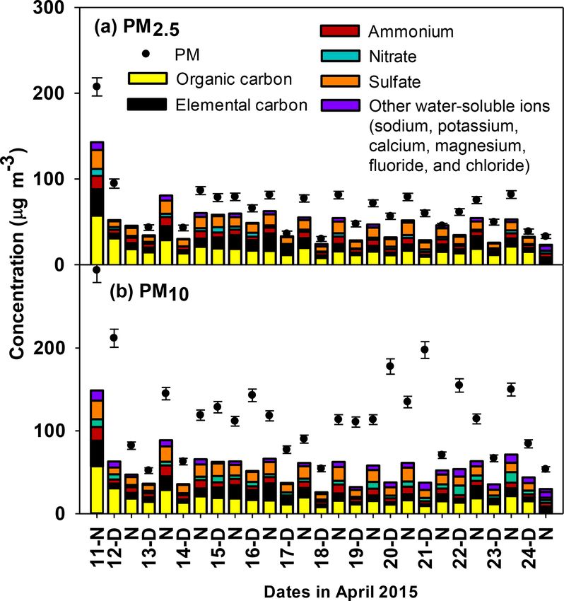
Md. R. Islam et al.: Ambient air quality in the Kathmandu Valley                                                               2931

on replicate analyses were approximately ±5 % of measured            and Cl− predicted by the model were used to calculate the
mixing ratios or ±0.5 times estimated detection limits (DL),         fractions of the measured concentrations that were ionized in
whichever were the greater absolute values. Due to sus-              aerosol solutions at ambient RH.
pected contamination of filter samples collected during 15              Equilibrium hydrogen ion activities for PM2.5 and PM10
to 17 April 2015 (described in Sect. 2.6), results for these         during each sampling interval were calculated based on
samples were excluded from the reported data set.                    the measured phase partitioning and associated thermody-
                                                                     namic properties of compounds with pH-dependent solubili-
2.8   Thermodynamic calculations                                     ties (HNO3 , NH3 , and HCl) following the approach of Keene
                                                                     and Savoie (1998). Briefly, using HNO3 as an example, the
Aerosol liquid water contents (LWCs), activity coefficients,         equilibrium
and the partitioning between ionized and solid aerosol con-
stituents were calculated using E-AIM (Extended Aerosol In-                      KH                 Ka
                                                                     HNO3 (g) ←→ HNO3 (aq.) ←→ H+ + NO−
                                                                                                      3                          (1)
organics Model) IV, which considers particles comprised of
                  2−
NH+         +              −     −
     4 , Na , SO4 , NO3 , Cl , and H2 O (Friese and Ebel,            was evaluated on the basis of simultaneous measurements of
2010) (http://www.aim.env.uea.ac.uk/aim/aim.php, last ac-            gas-phase HNO3 mixing ratios and particulate NO−      3 concen-
cess: 21 January 2020). E-AIM requires that the input data           trations in air; temperature-adjusted Henry’s Law (KH ) and
for ionic composition be balanced on an equivalent basis             acidity (Ka ) constants for HNO3 (Young et al., 2013); and
(i.e., 6 cations = 6 anions). Unmeasured ionic constituents          aerosol LWCs, NO−     3 activity coefficients, and the fractions
(e.g., carboxylic anions such as oxalate), ionic constituents        of measured particulate NO−    3 concentrations that were ion-
that were measured but are not considered by E-AIM (e.g.,            ized as predicted by E-AIM (described above).
K+ , Mg2+ , and Ca2+ ), and random analytical errors intro-             Although all concentrations of particulate Cl− were
duce minor ion imbalances into the subsets of input data. To         greater than estimated detection limits, most mixing ratios
balance an anion deficit for a given sample, the input concen-       (75 %) for volatile inorganic Cl were less than the detection
trations of SO2−        −         −
                4 , NO3 , and Cl were increased in proportion        limit and the balance of measurements was near the detection
to their measured concentrations on an equivalent basis. Sim-        limit. Consequently, the phase partitioning of HCl and as-
ilarly, to balance a cation deficit, concentrations of NH+   4 and   sociated data interpretations were poorly constrained. How-
Na+ were increased in proportion to their measured concen-           ever, NH3 , HNO3 , particulate NH+                            −
                                                                                                           4 , and particulate NO3
trations. Because the ionic compositions of aerosol sampled          were present at concentrations well above the corresponding
                                2−
were dominated by NH+                   −        −
                          4 , SO4 , NO3 , and Cl , these adjust-     detection limits and, as described in Sect. 3.2.4 below, the
ments in measured concentrations were relatively minor (typ-         measured gas–aerosol phase partitioning of NH3 and HNO3
ically < 15 % for a given analyte). Sensitivity studies indicate     yielded paired estimates of aerosol solution pHs that agreed
that alternative approaches to charge balance input data for         well (generally within ±0.1 to ±0.3 pH units). In the absence
E-AIM yield similar results (e.g., Young et al., 2013).              of direct reliable measurements of HCl, the equilibrium mix-
   For each sample, the input data included the measured (or         ing ratio for HCl during each sampling interval (hereafter re-
adjusted as described above) concentrations of NH+              +
                                                          4 , Na ,   ferred to as HClcalc ) was estimated using the same thermody-
    2−       −        −
SO4 , NO3 , and Cl and the corresponding temperature and             namic approach described above based on the mean H+ ac-
RH averaged over the sampling interval. Model output used            tivity inferred from the measured phase partitioning of NH3
for subsequent calculations included aerosol LWC; activity           and of HNO3 , the Cl− concentration for PM2.5 , the thermo-
coefficients for NH+          −        −
                      4 , NO3 , and Cl ; and, for mixed-phase        dynamic properties of HCl, meteorological conditions, the
particles, the partitioning of NH4 , NO−
                                     +                 −
                                           3 , and Cl between        aerosol LWC, Cl− activity coefficient, and fraction of mea-
dissolved and solid phases. E-AIM simulated three distinct           sured particulate Cl− that was ionized as predicted by E-
regimes: (1) at RH greater than about 75 %, the aerosol was          AIM.
completely deliquesced (i.e., virtually all NH+             −
                                                   4 , NO3 , and        Results based on the above approach are subject to sev-
   −
Cl were ionized); (2) at RH less than about 60 %, parti-             eral inherent limitations. (1) As indicated above, E-AIM IV
cles existed entirely as solids with only tightly bound wa-          evaluates only a subset of major inorganic constituents. Be-
ter molecules and negligible LWC; (3) at RH between about            cause potential influences of organic matter on aerosol hy-
60 % and 75 %, constituents partitioned between dissolved            groscopic properties are not considered, the modeled esti-
and solid (primarily (NH4 )2 SO4 ) phases. The extraction of         mates of water contents may diverge to some extent from
aerosol samples into dilute aqueous solutions prior to anal-         those in ambient air. However, as mentioned above, paired
ysis would have dissolved any solid phases that were orig-           independent estimates of aerosol solution pH based on the
inally present in particles at ambient LWCs. Consequently,           phase partitioning of HNO3 and of NH3 and corresponding
the measured concentrations of ions in dilute aerosol extracts       meteorological conditions measured simultaneously yielded
correspond to the total concentrations (ionized + solid) that        similar results. These two compounds have distinct ther-
existed in ambient aerosol prior to extraction. In these cases,      modynamic properties and associated pH-dependent solu-
the ratios of ionized to total (ionized + solid) NH+            −
                                                         4 , NO3 ,   bilities; the solubility of HNO3 decreases, whereas that of

www.atmos-chem-phys.net/20/2927/2020/                                                 Atmos. Chem. Phys., 20, 2927–2951, 2020
2932 Md. R. Islam et al.: Ambient air quality in the Kathmandu Valley
NH3 increases with decreasing solution pH. The good agree- mospheric constituents, associated aerosol acidities, and pH-
ment between the paired results suggests that estimates of dependent chemical transformations in the Kathmandu Val-
aerosol pH during the campaign were relatively insensi- ley.
tive to potential influences of organic matter on water con-
tents. (2) PM2.5 and PM10 were collected in bulk over rela- 2.9 Extraction and analysis of organic species in PM2.5
tively long (nominally 12 h) sampling intervals, which could by gas chromatography mass spectrometry
have driven artifact phase changes of compounds with pH-
dependent solubilities and associated bias in the measured All glassware used in solvent extraction was prewashed with
gas and particle phases species concentrations. For exam- ultrapure water and baked at 500 ◦ C for 5.5 h. Based on the
ple, based on their thermodynamic properties, NH3 parti- OC loading on the filters, one or more QFF for each time pe-
tions preferentially with the more highly acidic, typically riod was extracted following the procedure described in Al-
smaller longer-lived aerosol size fractions, whereas HNO3 Naiema et al. (2015). Organic species were analyzed using
and HCl partition preferentially with less acidic, typically gas chromatography coupled to mass spectrometry (GC-MS,
larger shorter-lived aerosol size fractions (Keene et al., 2004; Agilent Technologies GC-MS 7890A) equipped with an Agi-
Young et al., 2013). When chemically distinct particles are lent DB-5 column (30 m × 0.25 mm × 0.25 µm) and electron
mixed together in a bulk PM2.5 or PM10 sample, the pH of ionization (EI) source with a temperature program described
the bulk mixture typically differs from that of the aerosol in Stone et al. (2012). All the measured species were field
size fractions with which these gases partitioned preferen- blank subtracted, and analytical uncertainties of the measure-
tially in ambient air, which drives artifact volatilization of ments were propagated from the standard deviation of the
NH3 as well as HNO3 and HCl (Keene et al., 1990; Young field blanks and 20 % of the measured concentration to con-
et al., 2013). (3) Similarly, mixing chemically distinct parti- servatively account for compound recovery from QFF. De-
cles sampled at different times over sampling intervals could tails of the extraction process and GC temperature program
drive artifact volatilization or condensation of gases. Expos- are provided in the Supplement (S1).
ing time-integrated aerosol samples to gas-phase mixing ra-
2.10 Quality control in chromatographic
tios that vary over sampling intervals can also drive arti-
measurements of PM
fact phase changes. Because of their large surface-to-volume
ratios, sub-micrometer-diameter particles rapidly equilibrate For every five ambient samples, one lab blank, one field
(in seconds to minutes) with interstitial gases and, conse- blank, and one spike recovery sample were analyzed for both
quently, are typically at or near thermodynamic equilibrium organic species and inorganic ions. Spike samples were pre-
with the gas phase (Meng and Seinfeld, 1996). In contrast, pared from blank filters spiked with known concentrations
larger particles equilibrate more slowly and may exhibit finite of analytes. These quality control samples were extracted
phase disequilibria (e.g., Keene and Savoie, 1998). The as- simultaneously with ambient samples. Spike recoveries, re-
sumption of thermodynamic equilibrium on which this anal- ported as percent, were calculated as the quotient of the lab
ysis is based may not be entirely valid for constituents as- blank-corrected measured concentration and spiked concen-
sociated primarily with larger aerosol size fractions. (4) In tration. Spike recoveries of all the reported chemical species
addition, the use of average values to characterize meteoro- were within ±20 % for the organic species and ±10 % for the
logical conditions over sampling intervals does not capture inorganic ions. Reproducibility and method detection limits
the full range of variability of the multiphase system. On for all the organic species are presented in Table S1 in the
most days, RH fell to minima less than 60 % during day- Supplement.
time and increased to maxima greater than 75 % at night.
Consequently, based on E-AIM, the actual hydration state of 2.11 Chemical mass balance modeling
particles varied from virtually dehydrated to virtually com-
pletely deliquesced conditions over most diel cycles. Pre- PM2.5 OC was apportioned to its contributing sources us-
sumably, between collection and recovery, the compositions ing the Environmental Protection Agency’s chemical mass
of aerosol deposits on sample filters exposed to ambient air balance (EPA-CMB) model (version 8.2) using molecular
also evolved in response to changing RH and temperature. If marker concentrations in ambient PM2.5 and source pro-
so, meteorological conditions at recovery times rather than files as model inputs. Source profiles for garbage burning
those averaged over sampling intervals may be more ap- (fire nos. 14A and 14B), open biomass burning (fire no. 39),
propriate metrics for evaluating phase partitioning and pH. biomass- and dung-powered traditional cooking stoves (fire
(5) Finally, the thermodynamic properties of gases consid- nos. 37, 38, 40, and 41) were drawn from NAMaSTE in
ered herein (particularly HCl) are associated with non-trivial 2015 (Jayarathne et al., 2018). Other primary and secondary
uncertainty that contributes to variability in results as dis- source profiles were drawn from the literature: vegetative
cussed by Young et al. (2013). Despite these limitations, detritus (Hildemann et al., 1991; Rogge et al., 1993), non-
the results provide useful insight regarding major processes catalyzed gasoline engines (Lough et al., 2007; Schauer et
that modulate gas–aerosol phase partitioning of major at- al., 2002), diesel engines (Lough et al., 2007), small-scale
Atmos. Chem. Phys., 20, 2927–2951, 2020 www.atmos-chem-phys.net/20/2927/2020/Md. R. Islam et al.: Ambient air quality in the Kathmandu Valley 2933
coal combustion (Zhang et al., 2008), isoprene, monoter- thropogenic sources, suggesting that multiple ethane sources
pene, and sesquiterpene-derived SOA (Kleindienst et al., contribute. CH4 is likely then to derive at least partially from
2007), and aromatic SOA from naphthalene and methyl- combustion and is not expected to derive from natural gas
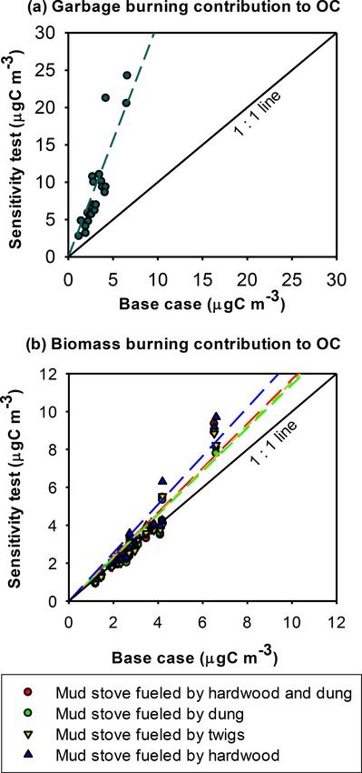
naphthalene (Kleindienst et al., 2012). The model sensitiv- production, processing, or transmission, due to a lack of natu-
ity to the input source profiles were evaluated by systemati- ral gas infrastructure in the Kathmandu Valley in 2015, aside
cally varying the biomass burning and garbage burning pro- from a small number of household-scale biogas plant sys-
files developed in NAMaSTE-2015 (Jayarathne et al., 2018), tems. Additionally, the presence of numerous outliers in the
which examined the following source profiles: open biomass data set suggests that individual grab samples were occasion-
burning, a mud stove fueled by wood and cow dung, a mud ally impacted disproportionately by local rather than regional
stove fueled by cow dung, a mud stove fueled by twigs, a sources (Table S2). The C3 -C5 alkanes are not major biomass
mud stove fueled by wood, and mixed garbage burning (sam- burning products but are associated with liquefied petroleum
ples A and B, discussed further in Sect. 3.6). gas (LPG) and gasoline (Guo et al., 2011). Their abundance
here suggests a traffic or fossil fuel source (as discussed in
2.12 Statistical analysis Sect. 3.1.2). In urban centers toluene often reflects traffic,
gasoline evaporation, and/or solvents (Ou et al., 2015; Tsai
The detectability of organic and inorganic species was et al., 2006). Four-stroke engines are abundant in the Kath-
100 %, except for 17α(H)-22,29,30-trisnorhopane (96 %), mandu Valley, and their emissions are rich in aromatic VOCs
17β(H)-21α(H)-30-norhopane (96 %), cholesterol (93 %), (Shrestha et al., 2013). Here toluene correlated best with
stigmasterol (89 %), 1-methylchrysene (93 %), stigmastanol C4 -C5 alkanes and ethylbenzene (r = 0.86 to 0.94) though
(67 %), retene (56 %), and coprostanol (30 %). Prior to statis- surprisingly poorly with the vehicle exhaust tracer ethene
tical analysis, data points with values below detection
√ limits (r = 0.01). While recognizing the limited sample size, this
were replaced with the limit of detection (LOD) / 2 (Hewett could suggest gasoline evaporation due to toluene’s correla-
and Ganser, 2007). All the concentrations were tested for tion with i-pentane (Tsai et al., 2006). Further study would
normality and lognormality using the Anderson–Darling test. help to clarify toluene’s sources.
Concentrations of all the species were either normally or log- Relative to previous measurements of NMVOC with a
normally distributed; thus Pearson’s correlation (r) was em- PTR-TOF-MS (proton transfer reaction time-of-flight mass
ployed for correlation analysis. Two sample t tests were used spectrometer) at Bode from December 2012 to January 2013
to compare the means of daytime and nighttime concentra- during the SusKat-ABC campaign (Sarkar et al., 2016), con-
tions. All statistical tests were performed in Minitab (ver- centrations of the NMVOCs listed in Table 3 were generally
sion 17) and significance was assessed at the 95 % confidence lower during NAMaSTE in April 2015. Seasonal variability
interval (p ≤ 0.05). in meteorology likely contributes to these differences. Mix-
ing layer depths and associated dilution of regional emissions
peak during the pre-monsoon season (March–May, includ-
3 Results and discussion
ing this study), whereas mixing layer depths are shallower
3.1 Abundance of VOC, CO2 , and CO during winter (Mues et al., 2017). Several rain events oc-
curred during April 2015 (specifically on 12 to 13, 15, 17
3.1.1 VOC abundance to 18, and 21 April) with a total of 24.2 mm of precipita-
tion. Associated scavenging would also have contributed to
Excluding oxygenated compounds, the 10 most abundant the lower pollution levels during this study relative to the dry
NMVOCs in descending order based on median values winter season characterized during the SusKat-ABC cam-
were ethene, ethyne, ethane, propene, propane, i-pentane, i- paign. Notably, isoprene levels were nearly 10 times lower
butane, n-butane, toluene, and m/p-xylene. These and other during April 2015 compared to the winter of 2012–2013.
selected NMVOC measurements in WAS are summarized in Sample collection in the early morning and late afternoon
Table 2, with the corresponding precisions, accuracies, and contributed to low isoprene concentrations in this study as
detection limits. Ethene and propene are major biomass burn- peak isoprene concentration is typically observed during the
ing products and major components of vehicle exhaust (Ak- midday (Karl et al., 2007). Previous studies report two pri-
agi et al., 2011; Guo et al., 2011), so their high abundance mary reasons for low isoprene emissions: (i) immaturity of
is expected given the prevalence of these sources. Ethyne is leaves, until reaching an age of 23 d (Kuzma and Fall, 1993)
a general combustion tracer that is expected to reflect vehic- and (ii) temperatures lower than 35 ◦ C (Monson et al., 1992).
ular, biomass, and biofuel combustion (Abad et al., 2011). By April, nearly all deciduous trees in the Kathmandu Valley
Ethane also has multiple major sources including fossil fuel have leaves, although spring 2015 was unusually cold and the
evaporation and combustion, biomass burning, and biofuel low temperatures leading up to and during the measurement
combustion (Guo et al., 2011; Xiao et al., 2008). Ethane period did not favor isoprene emissions as further discussed
correlated most strongly with the combustion tracer ethene in Sect. 3.2.6. The whole-air sampling in this study provides
(r = 0.81) and with CH4 (r = 0.66), which has many an- additional chemical detail to the high time resolution mea-
www.atmos-chem-phys.net/20/2927/2020/ Atmos. Chem. Phys., 20, 2927–2951, 20202934 Md. R. Islam et al.: Ambient air quality in the Kathmandu Valley
Table 2. Means, standard deviations, medians, and ranges of concentrations of methane, CO, CO2 , carbonyl sulfide (COS), and select non-
methane volatile organic compound (NMVOC) mixing ratios measured at Bode in April 2015 (n = 9). Species reported here include the 20
most abundant species, with all NMVOC measurements provided in Table S1. Units are in parts per billion by volume, unless noted.
Compound Precision (%) Accuracy (%) Mean ± SD Median Range
CH4 (ppmv) 0.1 1 1.999 ± 0.082 1.976 1.926–2.188
CO (ppmv) 2 5 0.766 ± 0.751 0.509 0.362–2.737
CO2 (ppmv) 2 2 425 ± 8 424 415–435
Carbonyl sulfide 2 10 0.66 ± 0.20 0.59 0.47–1.13
CH3 Cl 5 10 0.87 ± 0.22 0.86 0.67–1.42
Ethane 1 5 2.29 ± 0.39 2.20 1.69–2.74
Ethene 3 5 3.20 ± 1.11 3.26 1.59–4.64
Ethyne 3 5 3.06 ± 1.46 2.68 1.51–6.31
Propane 2 5 2.05 ± 1.69 1.39 0.69–5.77
Propene 3 5 1.92 ± 1.04 1.68 0.54–3.51
i-Butane 3 5 1.47 ± 0.97 1.29 0.28–3.21
n-Butane 3 5 1.39 ± 0.80 1.27 0.23–2.47
i-Butene 3 5 0.93 ± 0.80 0.82 0.12–2.81
1,3-Butadiene 3 5 0.13 ± 0.09 0.17 0.02–0.28
i-Pentane 3 5 1.77 ± 1.76 1.38 0.10–6.07
n-Pentane 3 5 0.46 ± 0.37 0.45 0.03–1.25
n-Hexane 3 5 0.29 ± 0.26 0.21 0.03–0.80
n-Heptane 3 5 0.24 ± 0.36 0.10 0.02–1.18
n-Octane 3 5 0.12 ± 0.08 0.09 0.05–0.30
n-Nonane 3 5 0.18 ± 0.14 0.16 0.04–0.42
Benzene 3 5 1.01 ± 0.49 0.86 0.59–2.19
Toluene 3 5 0.99 ± 0.53 1.06 0.30–1.84
m/p-Xylene 3 5 1.11 ± 0.61 1.02 0.20–2.26
o-Xylene 3 5 0.46 ± 0.29 0.40 0.13–0.89
Methanol 30 20 4.38 ± 1.66 3.94 2.82–7.98
Ethanol 30 20 4.34 ± 2.36 3.97 1.51–9.85
Acetaldehyde 30 20 5.24 ± 4.17 3.53 1.56–15.15
Butanone 30 20 0.98 ± 1.05 0.71 0.00–3.63
Isoprene 3 5 0.11 ± 0.07 0.09 0.06–0.24
α-Pinene 3 5 0.11 ± 0.12 0.05 0.03–0.30
β-Pinene 3 5 0.09 ± 0.07 0.06 0.02–0.18
6 measured NMVOC n/a n/a 48 ± 19 45 25–83
n/a: not applicable.
surements by PTR-TOF-MS during the SusKat-ABC inten- CO2 concentrations in Kathmandu are elevated above the
sive campaign (Sarkar et al., 2016), including the resolution global background (Table 2). CO (like the NMVOCs and
of alkane and aromatic VOC isomers, chlorofluorocarbons, PM) is an excellent indicator of air pollution levels and
and alkyl nitrates (Table S2). is derived from combustion rather than solvents or sec-
In comparison to other cities in South Asia (Table 3), the ondary sources. As shown in Table 3, the pattern of CO en-
NMVOC levels observed in Kathmandu were 1.3 to 8.5 times hancements relative to other studies is similar to the pattern
lower than in Mohali, India (Sinha et al., 2014), 2.6 to 6.7 for most NMVOCs. The three studies in Kathmandu during
times lower than in Karachi, Pakistan (Barletta et al., 2002), the dry season have similar values to each other. The impor-
9.5 to 33 times lower than in heavily polluted Lahore, Pak- tance of combustion as a source of air pollutants, particularly
istan (Barletta et al., 2017), and about a factor of 2 higher PM, is consistent with the carbon mass balance source ap-
than in Singapore (Barletta et al., 2017). Bearing in mind portionment results discussed in Sect. 3.3.
the small sample size, the observed NMVOC levels in Kath-
mandu indicate that in April 2015, it was moderately polluted 3.1.2 VOC sources
with respect to other South and Southeast Asian cities, with
relatively low biogenic VOC influences. Because the NMVOC data set is too small (n = 9) to be used
in source apportionment techniques like positive matrix fac-
torization (PMF), we use VOC ratios to further probe source
Atmos. Chem. Phys., 20, 2927–2951, 2020 www.atmos-chem-phys.net/20/2927/2020/Table 3. Comparison of mean concentrations of select volatile compounds measured during this study with those measured during prior studies in the Kathmandu Valley and cities in
South and Southeast Asia. Units are in parts per billion by volume.
Location and dates Kathmandu, Kathmandu, Kathmandu, Mohali, Karachi, Lahore, Singapore Mecca, Saudi
www.atmos-chem-phys.net/20/2927/2020/
Nepal Nepal Nepal India Pakistan Pakistan Arabia
Compound Apr 2015 Dec 2012–Jan 2013 Apr 2013 May 2012 Dec 1998–Jan 1999 Dec 2012 Aug–Nov 2012 Oct 2012
CO 770 (750) 832 (422)a,b 700 (–c ) 567 (293) 1600 (1300) 4860 (690)d 280 (11) 2230 (380)
CH4 2000 (80) 2550 (120)a 2183 (252) – 6300 (4700) 5380 (440)d 1822 (6) 1880 (8)
Acetaldehyde 5.2 (4.2) 8.8 (4.6) – 6.7 (3.7) – – – –
Methyl chloride 0.9 (0.2) – – – 2.7 (1.5) – – –
Methanol 4.4 (1.7) 7.4 (1.3) – 37.5 (17.9) – – – –
Ethanol 4.3(2.4) 1.6 (0.8) – – – – – –
Propene 1.9 (1.0) 4.0 (1.2) – – 5.5 (5.3) 18.3 (3.0)d 0.8 (0.2) 5.5 (1.3)
Benzene 0.9 (0.5) 2.7 (1.2) – 1.7 (1.5) 5.2 (4.5) 28.2 (4.8)d 0.58 (0.06) 4.5 (1.1)
Md. R. Islam et al.: Ambient air quality in the Kathmandu Valley
Toluene 1.1 (0.5) 1.5 (0.4) – 2.7 (2.9) 7.1 (7.6) 32.4 (6.0)d 1.8 (0.3) 7.3 (1.6)
Xylenes 1.6 (0.7) 1.0 (0.3) – 2.0 (2.2) 4.2 (2.4) 23.2 (3.5)d 0.9 (0.1) 5.0 (0.6)
Isoprene 0.11 (0.07) 1.1 (0.2) – 1.9 (0.9) 0.8 (1.1) 1.3 (0.2)d 0.27 (0.02) 2.0 (0.5)
i-pentane / n-pentane 4.7 – – – 0.9 1.3 1.9 3.52
Ethene / ethyne 0.5 – – – 1.1 0.91 1.1 0.73
i-butane / n-butane 1.1 – – – 0.53 0.56 0.62 0.44
Number of samples 9 NAe NAf NAe 78 41 85 72
Reference This study Sarkar et al. (2016) Mahata et al. (2018) Sinha et al. (2014) Barletta et al. (2002) Barletta et al. (2017) Barletta et al. (2017) Simpson et al. (2014)
a Data from Bhardwaj et al. (2018). b Monthly average for January 2013. c Dash denotes data not available. d Standard error. e NMVOC were measured continuously by PTR-MS. f CO and CH were measured continuously.
4
Atmos. Chem. Phys., 20, 2927–2951, 2020
29352936 Md. R. Islam et al.: Ambient air quality in the Kathmandu Valley
influences. All NMVOC ratios cited herein have been re-
ported previously by Simpson et al. (2014) and references
therein, Akagi et al. (2011), and Stockwell et al. (2016). The
ratio of i-pentane / n-pentane increases from ∼ 1 for natu-
ral gas to ∼ 4 for gasoline evaporation. Here, the ratio was
4.7 ± 0.4 (r = 0.97), consistent with gasoline evaporation as
has been seen in other cities such as Mecca, Saudi Arabia
(Simpson et al., 2014). The diurnal ambient temperature dur-
ing this study ranged from 12 to 29 ◦ C, which is conducive to
evaporation. As in Mecca, fuel pump hoses in the Kathmandu
Valley are not equipped with vapor recovery technology and
vehicles are not equipped with catalytic converters, which
may partially explain the abundance of the gasoline evapo-
ration tracer i-pentane. Ethene/ethyne can be used to differ-
entiate petrochemical sources (10–30) from biomass burning
(2–5) and vehicle exhaust (1–3), with ratios below 1 reflect-
ing older emissions control technology due to higher ethyne
emissions. Here the ratio was 0.5, similar to Saudi Arabia
(0.73), suggesting a very large impact of older or poorly
maintained vehicles (Zhang et al., 1995). The i-butane / n-
butane ratio can sometimes help to distinguish influence from
vehicles (∼ 0.2 to 0.3), LPG combustion (∼ 0.42 to 0.46),
and natural gas leaks (∼ 0.6 to 1.0). Here the butane ratio
Figure 1. Non-water mass concentrations of (a) PM2.5
was relatively high (∼ 1, r 2 = 0.90) as compared to cities in and (b) PM10 during daytime and nighttime periods and mass
Saudi Arabia and Pakistan (0.4 to 0.6; Barletta et al., 2017; contributions from OC, EC, and inorganic ions. OC and EC were
Simpson et al., 2014). The cause of the relatively abundant not measured in PM10 samples and were assumed to be the same
i-butane could be a mix of sources, such as non-evaporative as PM2.5 for mass balance purposes. The remaining mass of PM2.5
liquid petroleum gas emissions (1.39), aged gasoline genera- includes elements associated with OC (hydrogen, oxygen, nitrogen,
tor (1.17), diesel generator (0.87), agricultural fires (0.93), or etc.), metals, and other unmeasured species. Error bars represent
zigzag kilns (0.84) (Stockwell et al., 2016), which requires propagated analytical uncertainties. The PM2.5 mass was not
further investigation. Acetaldehyde was a major NMVOC quantified for nighttime samples collected on 12 April nor 13 April
consistent with past work (Table 3), and it has a variety of as described in Sect. 2.2.
poorly constrained primary and secondary sources (Akagi
et al., 2011; Stockwell et al., 2016). These observations are
consistent with the PMF analysis of NMVOC measurements 68.2 ± 34.7 µg m−3 . PM10 mass concentrations ranged from
during the SusKat-ABC intensive campaign, which indicated 51.9 to 294.0 µg m−3 and averaged 119.7 ± 55.2 µg m−3 .
that traffic and industrial emissions were the largest sectors All of the 11 h PM2.5 and PM10 concentrations exceed
contributing to NMVOC mass loadings, at 17 % and 18 %, the World Health Organization (WHO) 24 h guidelines of
respectively (Sarkar et al., 2017). The large diversity of com- 25 and 50 µg m−3 , respectively. The maximum concentra-
bustion emissions in Kathmandu, the apparent influence of tions of PM2.5 and PM10 occurred during the night of
point NMVOC sources, and chemical signatures not previ- 11 April (Fig. 1), concurrent with the Bisket Jatra festival;
ously observed in South Asia (discussed above) indicate that see Sect. 3.4 for a detailed description of this pollution event
additional research with a larger sampling size is needed to and its source characteristics.
better understand NMVOC sources in the Kathmandu Val- The average PM2.5 concentration observed in this study
ley. Such research is ongoing as part of our second Nepal is about half the mean 24 h average PM2.5 concentration
Ambient Monitoring and Source Testing Experiment (NA- near six major road intersections in the Kathmandu Val-
MaSTE2). ley (which averaged 125 ± 56 µg m−3 ) during the relatively
drier period February–April 2014 (Shakya et al., 2017b). The
3.2 Particulate matter and inorganic trace gases average PM2.5 concentration in the Kathmandu Valley was
about a factor of 2 higher than at a more rural and cleaner
3.2.1 PM2.5 and PM10 concentrations foothill site at Godawari (34 µg m−3 ) during April 2006
(Stone et al., 2010) and about a factor of 13 higher than
PM2.5 mass concentrations averaged over 11 h at the Bode the PM1 concentration (5.4 µg m−3 ) at the Nepal Climate
supersite from 11 to 24 April 2015 ranged from 30.0 to Observatory-Pyramid (NCO-P) site (near the base camp for
207.4 µg m−3 (Fig. 1) and averaged (± standard deviation) Mt. Everest) in the southern Himalaya (27.95◦ N, 86.82◦ E)
Atmos. Chem. Phys., 20, 2927–2951, 2020 www.atmos-chem-phys.net/20/2927/2020/Md. R. Islam et al.: Ambient air quality in the Kathmandu Valley 2937
during March–April 2006 (Bonasoni et al., 2008). The aver-
age PM10 concentration in the Kathmandu Valley observed
in this study period is similar to the average concentration
(155 ± 124 µg m−3 ) of total suspended particles at Bode be-
tween April 2013 and March 2014 (Chen et al., 2015).
PM concentrations at Bode were consistently higher dur-
ing nighttime (83 µg m−3 for PM2.5 and 121 µg m−3 for
PM10 ) compared to daytime (54 µg m−3 for PM2.5 and
117 µg m−3 for PM10 ). The high time resolution data for the
AMS total signal (Fig. 2) indicate that PM mass increases
overnight, peaks around 08:00 local time, and thereafter de-
creases to minima around 17:00. Diurnal variability in PM
loadings is attributed to four interrelated factors. (1) Bound-
ary layers and the corresponding volumes of air into which
pollutants are emitted are relatively shallower at colder noc-
turnal temperatures (Mues et al., 2017). Although vertical
temperature profiles were not measured, the Kathmandu Val-
ley frequently experiences shallow nocturnal inversion as ev-
ident in ceilometer measurements during the SusKat-ABC
campaign (Mues et al., 2017). (2) Wind speeds during the Figure 2. Diurnal trends in average total PM1 mass and concentra-
pre-monsoon season and the corresponding dilution of PM tions of non-refractory inorganic species measured with the AMS,
emitted into or produced within that air flow are typically average BC measured with the aethalometer, and average wind
speed and direction at Bode on 13 and 16 to 24 April 2015. The
lower at night (< 1 m s−1 ) relative to daytime (1 to 5 m s−1 )
shaded region represents the duration for nighttime filter collection
(Fig. 2). The afternoon increase in wind speed corresponds and the unshaded region represents the duration for daytime filter
to minimum PM values, while lower wind speeds in early collection.
evening coincide with higher concentrations. (3) The diur-
nal wind dynamics in the Kathmandu Valley have been pre-
viously described (Mahata et al., 2017; Panday and Prinn, organic matter (OM) were estimated by multiplying OC mass
2009; Panday et al., 2009; Sarkar et al., 2016). From midday concentrations by a factor of 1.7 to account for the associ-
to dusk, strong westerly flows carry pollutants from Kath- ated elements (primarily oxygen, hydrogen, and nitrogen).
mandu and Lalitpur towards the east and south passes of the The OM : OC conversion factor of 1.7 was obtained from the
valley, and the mixing layer height reaches its maximum. AMS measurement and falls towards the urban end of the
During evening, relatively stagnant cooler air causes pollu- range (1.6–2.1) recommended by Turpin and Lim (2001).
tants from the Bhaktapur Industrial Estate (which includes OM accounted for an average of 48±9 % of PM2.5 mass. EC
∼ 19 biomass- and coal-fired brick kilns) located within 1 concentrations ranged from 2.3 to 30.8 µg m−3 (averaging
to 5 km of Bode to accumulate near the surface, with slight 9.0±6.4 µg m−3 ) and accounted for 13±6 % of PM2.5 mass.
elevation due to mild downslope flows. In the early morn- Major sources for OC and EC are discussed in Sect. 3.3.
ing, elevated pollutants briefly recirculate back to the surface.
Later in the morning, upslope flows loft polluted air prior to 3.2.3 Inorganic ions in PM, trace gases, and
the emergence of the strong westerly winds. (4) As discussed gas–aerosol phase partitioning
in more detail below, diel variability in temperature and RH
drove corresponding diel variability in aerosol liquid water The major ionic components of PM2.5 were sulfate, ammo-
content, aerosol solution pH, and the gas–aerosol phase par- nium, and nitrate accounting for 16±4 %, 9±3 %, and 4±2 %
titioning of compounds with pH-dependent solubilities. The of PM2.5 and 11±3 %, 6±2 %, and 3±2 % of PM10 , respec-
higher RHs and aerosol liquid water contents at night shifted tively (Table S3). Ratios of these ions indicate that secondary
partitioning towards the particulate phase, thereby contribut- inorganic compounds including ammonium sulfate and am-
ing to relatively higher PM mass concentrations at night. All monium nitrate were important components of PM (Carrico
of the above factors contribute to the relatively higher PM et al., 2003). The relative abundances of these species in the
concentrations in near-surface air at Bode during nighttime. Kathmandu Valley are within the ranges of those reported
previously (Shakya et al., 2008, 2010, 2017a).
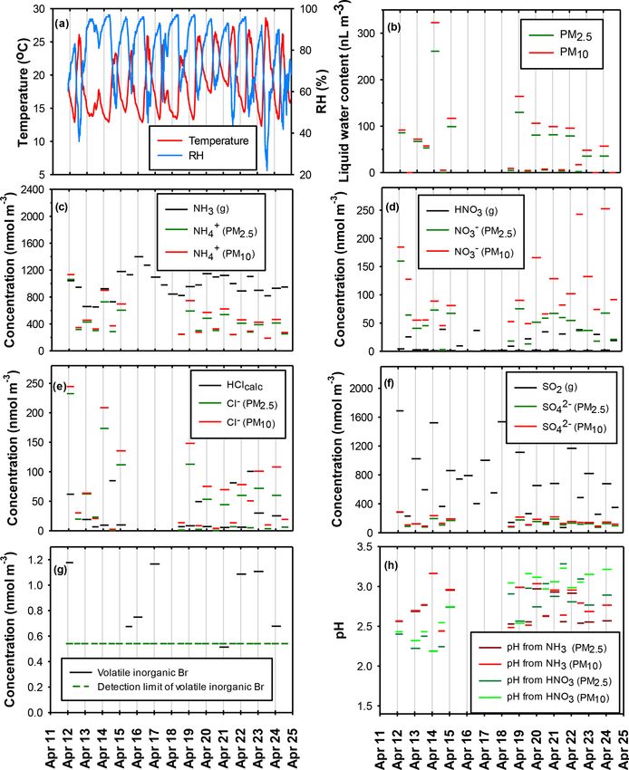
3.2.2 PM2.5 organic and elemental carbon Large diel variability in temperature and RH drove cor-
responding variability in aerosol LWC, which contributed
OC concentrations ranged from 7.9 to 57.3 µg C m−3 (aver- to diel variability in the phase partitioning of NH3 /NH+ 4,
aging 17.6 ± 9.6 µg C m−3 ) and accounted for 26 ± 5 % of HNO3 /NO− 3 , and HCl/Cl −
and aerosol solution pH (Fig. 3).
total PM2.5 mass. The corresponding mass concentrations of In contrast, under acidic conditions (as existed during this
www.atmos-chem-phys.net/20/2927/2020/ Atmos. Chem. Phys., 20, 2927–2951, 20202938 Md. R. Islam et al.: Ambient air quality in the Kathmandu Valley campaign; see below) and in the presence of high aerosol 1.18 nmol m−3 and were greater than the detection limit in 8 surface area, SO2 and H2 SO4 are relatively insensitive to the of 27 samples (Fig. 3g). Seven of the eight detectable mixing variability of aerosol LWC and solution pH. Under these con- ratios were during nighttime sampling intervals, which sug- ditions, virtually all SO2 partitions into the gas phase and vir- gests a possible diel cycle in multiphase chemical processing tually all H2 SO4 partitions into the particulate phase. Conse- of volatile Br and/or systematic variability as a function of quently, the phase partitioning of oxidized S (Fig. 3f) can be transport from different source regions. Br− was not mea- interpreted without complications introduced by correspond- sured in aerosol samples, so the corresponding variability of ing phase changes in response to variable LWC and pH. particulate and total (volatile + particulate) Br is not known. Both SO2 and particulate SO2− 4 were systematically higher Possible sources for reactive Br in the region include biomass at night and lower during the daytime (Table 4, Fig. 3f). The burning and fossil fuel combustion (Sander et al., 2003). average concentration of particulate SO2− 4 measured with the Concentrations of volatile and particulate inorganic Cl AMS followed a similar day–night trend, with peak concen- measured at Bode fell within the ranges of those mea- trations occurring around 08:00 local time (Fig. 2). The cor- sured in polluted continental air (Young et al., 2013). In responding total oxidized S (SO2 + particulate SO2− 4 ) dur- addition, concentrations of volatile inorganic Br and Cl at ing daytime versus nighttime (Table 4) typically differed by Bode fell within the ranges of those measured in marine air factors of 2 to 5. If the photochemical oxidation of SO2 (Keene et al., 2009; Sander et al., 2003). The lack of rele- to H2 SO4 had contributed significantly to the diel variabil- vant ancillary measurements during the period of the cam- ity in SO2 , SO2 and particulate SO2− 4 would have been an- paign precluded a quantitative assessment of the potential ticorrelated, which was not the case. These results imply impacts of reactive halogens on regional air quality in the that diel variability in atmospheric dynamics (wind velocity, Kathmandu Valley. However, drawing on related measure- boundary layer depth, and transport of chemically distinct air ments and model calculations elsewhere (Keene et al., 1999, masses within the valley, such as air masses with brick kiln 2009; Long et al., 2014; Sander et al., 2003; Young et al., influence at night) were major drivers of the observed vari- 2013), our results in conjunction with the presence of acidic, ability in both species as discussed in Sect. 3.2.1. deliquesced aerosol support the hypothesis that multiphase Total NH3 (NH3 + particulate NH+ 4 ) exhibited a diel pat- halogen-radical chemistry involving both Br and Cl impacted tern similar to that of oxidized S (Table 4, Fig. 3c) al- air quality via two pathways. (1) At high NOx mixing ra- though relative day–night differences were proportionally tios in polluted continental regions, the nocturnal reaction smaller (typically less than a factor of 2). Day–night dif- of N2 O5 with particulate Cl− produces significant ClNO2 , ferences in total NO3 (HNO3 + particulate NO− 3 ) and total which photolyzes following sunrise yielding a burst of Cl Cl (HClcalc + particulate Cl− ) (Table 4, Fig. 3d and e, re- atoms (e.g., Brown et al., 2013). ClNO2 is also a noctur- spectively) were somewhat more variable but also tended nal reservoir for NOx and thereby slows NOx destruction to be higher at night than during the day. Taken together, at night. (2) The scavenging of volatile HOCl and HOBr the above results support the hypothesis that the transport into acidic aerosol solution and their subsequent reaction of chemically distinct air masses from different source re- with Cl− and Br− produces Cl2 , BrCl, and Br2 , which sub- gions during daytime versus nighttime was a major factor sequently volatilize to the gas phase and photolyze during that drove diel variability in the composition of the multi- daytime yielding atomic Br and additional atomic Cl (e.g., phase gas–aerosol system at Bode. Concentrations of Na+ Keene et al., 2009). These autocatalytic reactions proceed in (in nmol m−3 ) associated with PM2.5 (median – 4.0, range both the light and dark and would enhance halogen activa- – undetectable to 19.0) and PM10 (median – 8.7, range – tion at night and sustain halogen-radical chemistry during undetectable to 40.9) were typically much lower than those daytime relative to predictions based on ClNO2 activation of particulate Cl− and total Cl (Fig. 3e). These relationships alone. The associated production and scavenging of halo- indicate that, in contrast to some other continental regions gen nitrates also accelerates the destruction of NOx . Cl and (e.g., Young et al., 2013; Jordan et al., 2016), refractory Br radicals contribute to the oxidation of hydrocarbons and, NaCl emitted from crustal and/or marine sources was not the together with related reactions that impact NOx cycling, per- primary source for particulate and volatile Cl at Bode. In- turb HOx –NOx photochemistry relative to that predicted in stead, total Cl (HClcalc + particulate Cl− ) showed high cor- the absence of reactions involving halogens. relation with potassium (r = 0.91, p
You can also read