An Analysis of Rhythmic Patterns with Unsupervised Learning - MDPI
←
→
Page content transcription
If your browser does not render page correctly, please read the page content below
applied
           sciences
Article
An Analysis of Rhythmic Patterns with
Unsupervised Learning
Matevž Pesek 1, * , Aleš Leonardis 1,2 and Matija Marolt 1
 1    Faculty of Computer and Information Science, University of Ljubljana, Vecna pot 113, 1000 Ljubljana,
      Slovenia; a.leonardis@cs.bham.ac.uk (A.L.); matija.marolt@fri.uni-lj.si (M.M.)
 2    School of Computer Science, University of Birmingham, University Rd W, Birmingham B15 2TT, UK
 *    Correspondence: matevz.pesek@fri.uni-lj.si

 Received: 18 October 2019; Accepted: 20 December 2019; Published: 25 December 2019

 Abstract: This paper presents a model capable of learning the rhythmic characteristics of a music
 signal through unsupervised learning. The model learns a multi-layer hierarchy of rhythmic patterns
 ranging from simple structures on lower layers to more complex patterns on higher layers. The
 learned hierarchy is fully transparent, which enables observation and explanation of the structure
 of the learned patterns. The model employs tempo-invariant encoding of patterns and can thus
 learn and perform inference on tempo-varying and noisy input data. We demonstrate the model’s
 capabilities of learning distinctive rhythmic structures of different music genres using unsupervised
 learning. To test its robustness, we show how the model can efficiently extract rhythmic structures in
 songs with changing time signatures and live recordings. Additionally, the model’s time-complexity
 is empirically tested to show its usability for analysis-related applications.

 Keywords: music information retrieval; rhythm analysis; compositional hierarchical model

1. Introduction
     Musical rhythm represents one of the basic elements of music. Several different aspects of rhythm
and its perception have been explored in the fields of psychology [1], musicology and music theory [2,3],
and music information retrieval (MIR) [4]. Rhythm is directly related to tempo [5]; moreover, rhythm
may affect and change the perception of tempo without changing the latter. Rhythmic patterns
significantly affect both the melodic and harmonic aspects of a music piece. By changing the underlying
rhythmic structure, two versions of a song may be classified into different music genres and imply
different dancing styles.
     Due to its importance, rhythm and its related concepts of tempo and beat have been extensively
explored in the music information retrieval field. In the following subsections, we present a cross
section of related works and then provide motivation for developing a new model, presented in
this paper.

1.1. Related Work
    In the field of music information retrieval, many rhythm, tempo, and beat related problems
have been explored. According to Bello et al. [4], there are several established perspectives on
musical rhythm. Four tasks are formalized within the Music Information Retrieval Evaluation
eXchange (MIREX) (http://www.music-ir.org/mirex/wiki/MIREX_HOME) [6]: genre estimation,
tempo estimation, beat tracking and downbeat estimation.

Appl. Sci. 2020, 10, 178; doi:10.3390/app10010178                                 www.mdpi.com/journal/applsci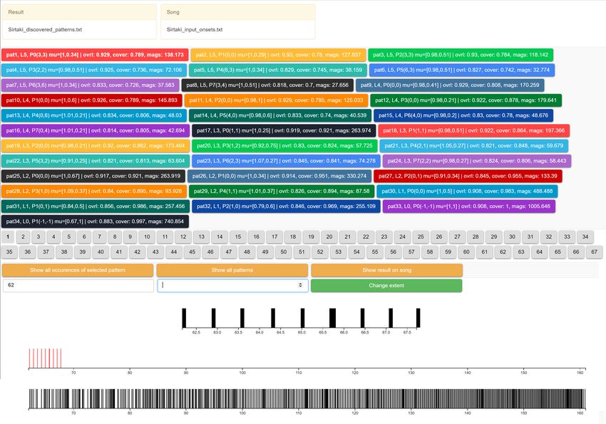
Appl. Sci. 2020, 10, 178                                                                            2 of 22

1.1.1. Established MIR Tasks
       The audio genre classification task is closely related to rhythm since rhythmic patterns represent
one of the key features for differentiation between music genres. For example, Dixon et al. [7] tackled
the problem of dance music genre classification by identifying different patterns, which define each
music genre. They evaluated their approach on the Ballroom music dataset, which contains eight
music genres: Jive, Cha cha, Quickstep, Rumba, Samba, Tango, Viennese Waltz and (English) Waltz.
They showed that the rhythmic patterns are a useful feature for genre classification. Esparza et al. [8]
proposed a neural network for rhythm genre classification and evaluated it on the Latin Music Dataset
where their approach achieved state of the art results. They further explored the underlying rhythmic
structures and pointed out several limitations in the dataset. Their research also showed that a single
genre is not necessarily defined by a single specific rhythm in dance music due to inter-genre influence.
       The tempo estimation task, as one of the first MIREX tasks, is also closely related to the rhythmic
aspect of music. In recent years, deep learning has been used for tempo estimation. For example,
Böck et al. [9] proposed an approach based on recurrent neural networks in combination with comb
filters. As a generalization of tempo estimation, the goal of beat tracking is to identify the positions
of beats in the audio. Although the task seems relatively trivial, current F-measures of the best
approaches on different datasets still only reach around 0.6–0.7 (MIREX 2018) [10,11]; therefore, there
is still room for improvement. The downbeat estimation task extends beat tracking by also identifying
the first beat of each measure. To reduce the dominance of 3/4 and 4/4 meters prevalent in Western
music, several non-Western music datasets (e.g., Turkish, Cretan and Carnatic) are used for evaluating
the algorithms for this task. Due to the strong interrelationship of meter, beat, and tempo, several
approaches attempt to model more than one aspect of rhythm. For example, Krebs et al. [12] proposed
a Hidden Markov model-based system, which they applied to beat tracking and downbeat estimation.
They also evaluated their system on the Ballroom dataset.

1.1.2. Models for Music Understanding
     Next to MIREX-type tasks, several researchers explored modeling of musical rhythm, where
the focus is on the model and understanding of the modeled structures. These models often rely on
analyses of human cognitive processes, and the perception of music and language.
     One of the more recently established and frequently used music theories was proposed by
Huron [13,14], based on six perceptual principles. He empirically shows that many of the commonly
known music rules have their basis in the perceptual principles. Inspired by Huron’s work, Abdallah
and Plumbley [15] proposed a simple Markov chain model for rhythm modeling, to explore
interconnections between entropy rate and aesthetic value. They applied the proposed model to
two pieces of minimalist music and showed that their rather simplistic model produces a similar
analysis to one provided by a human expert. Sioros et al. [16] proposed a generative model for
characterization of musical rhythms by using transformations, which provide a musically meaningful
encoding of patterns, focusing on the syncopation in rhythmic patterns. The model incorporates
Huron’s metrical expectation principle of weak–strong bonds to model syncopation. The authors
demonstrated the model’s performance on a pop music piece by Michael Jackson. They argue the
proposed model’s explicitness and usability for analysis, by providing “musically and perceptually
meaningful and detailed characterization” (p. 126). The proposed model extends beyond the analysis
of rhythm with its generative nature.
     In contrast to models based on human perception, data-driven models learn implicit rules by
extracting knowledge from large datasets. For example, Foscarin et al. [17] proposed a model based on
probabilistic context-free grammars trained on quantized MIDI files from music21 (http://web.mit.
edu/music21/doc/about/referenceCorpus.html) and EWLD [18] datasets. Starting with unweighted
acyclic grammars, this approach builds minimal parse trees from the music input. By adding additional
restrictions and limiting the amount of all possible rules to be learned from the input, the model
produces meaningful representations of rhythm structure and rhythmic notation.
Appl. Sci. 2020, 10, 178                                                                         3 of 22

     Temperley [19] proposed a unified model for polyphonic music analysis, including metrical
analysis. In this later work, Temperley [20] focused on the rhythmic modality and compared six
probabilistic models of rhythm on two datasets, the Essen Folksong Collection, and the corpus of
Mozart and Haydn string quartets, to explore ways of modelling rhythm perception. The author
argues that the perception of common-practice rhythm is governed by general principles. There are
several hypotheses discussed, each arguing one of the six models presented: the Uniform Position
Model, the Zeroth-Order Duration Model, the Metrical Position Model, the Fine-Grained Position
Model, the First-Order Metrical Duration Model and the Hierarchical Position Model. The latter is
based on the hypothesis that “the common-practice rhythms are generated in a hierarchical manner”
(p. 358). Among the six models, the Hierarchical Position Model and the First-Order Metrical Duration
Model achieved the lowest cross-entropy, with the Hierarchical Position Model being severely less
complex than the First-Order Metrical Duration Model.
     Since rhythm in non-Western music contains a more extensive variety of different meters,
several works are explicitly dedicated to exploration and rhythm modeling of non-Western music.
Holzapfel [21] observed the rhythmic patterns (usul) in Turkish Makam music. He investigated how
these patterns are related to note events and how the patterns are related to the meter as a latent
mental construct. By investigating the rhythmic patterns in a large corpus of Turkish music, he
proposed a methodology capable of identifying the differences between Western and Turkish music,
and applied a maximal likelihood criterion for rhythm classification. Similarly, London et al. [22]
explored African rhythmic patterns, focusing on three different music rhythms. In their study, they
explore the complexity of the perceptual and cognitive relationships between rhythmic patterns and
their interpretive metric frameworks. They also compared their data to the Turkish Makam music [21].
Panteli and Dixon [23] investigated the invariance of audio features for a description of rhythmic
content of diverse music styles, including Afro-American, North-Indian, African, Latin-Brazilian and
classical music styles.

1.2. Motivation
     The aforementioned approaches range from theoretical models for music understanding,
to automatic methods for classification and estimation of rhythmic events in audio and symbolic
music representations. While the classification models often give adequate results for a specific task,
they seldom focus on the perceptual and cognitive aspects of rhythm. Often, they are designed as
black boxes (e.g., using neural networks), which are trained for the task, but have limited ability to
investigate and explain the learned concepts. When trained through a supervised or unsupervised
procedure, large datasets are needed, which are often difficult to obtain, especially when dealing
with non-mainstream or non-Western music. On the other hand, the theoretical and cognitive
models attempt to encapsulate the perceptual and cognitive processes but are more challenging
to evaluate. Usually, a significant amount of music knowledge is built into these models by design,
without a learning process. Therefore, while they may deliver feasible and human-understandable
explanations of the underlying cognitive concepts, these approaches often operate as immutable
systems, constrained by the embedded knowledge.
     To bridge the gap between both types of approaches, we propose an unsupervised learning
approach for modeling rhythm. The model is derived from the compositional hierarchical model
(CHM) that was previously applied to tasks such as multiple fundamental frequency estimation [24]
and pattern discovery from symbolic music representations [25]. The presented model—the
compositional hierarchical model for rhythm analysis (RhythmCHM)—unsupervisedly learns a
multi-layer hierarchy of rhythmic patterns ranging from simple structures on lower layers to more
complex pattern compositions on higher layers. The learned hierarchy is fully transparent, which
enables the structure of the learned patterns to be observed and explained. The model employs
tempo-invariant encoding of patterns and can thus learn and perform inference on tempo-varying and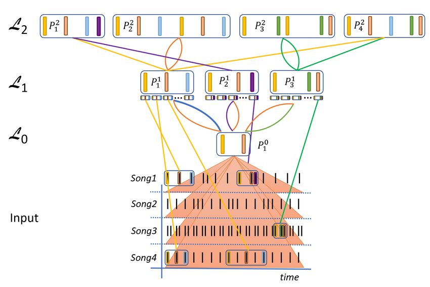
Appl. Sci. 2020, 10, 178 4 of 22
noisy input data. It does not carry any predefined notions on the underlying musical meters and can
perform on any type of (rhythmic) music.
Due to its transparency, the model can be used as an analytical tool for musicologists to aid
the pattern discovery and analysis. Additionally, the output of the model—pattern occurrences,
frequencies and their hierarchical structures—can be used as features for classification with machine
learning [26]. In contrast to other theoretical or symbolic-input models, the proposed approach robustly
models changes in rhythm, which are more common in non-popular music, and successfully models
tempo variations in live music. The model can therefore aid the researchers in music-related fields,
such as (ethno)musicology and music information retrieval.
The paper is structured as follows: in Section 2, we present the RhythmCHM focusing on its
structure and incorporated mechanisms. In Section 3, we analyze the model’s performance from several
viewpoints: its ability to learn patterns which are unique to individual music genres, its performance
on pieces with different meters and its robustness to varying tempo and variations present in live
music. The model’s scalability and time complexity are also explored. We conclude the paper in
Section 5 with a discussion of the performed experiments and ideas for future work.
2. The Compositional Hierarchical Model for Rhythm Modeling
In this section, we present the compositional hierarchical model for rhythm modeling
(RhythmCHM). The compositional hierarchical model for music information retrieval was first
introduced by [27] and has been applied to several MIR tasks, including automated chord estimation
and multiple fundamental frequency estimation [24], as well as finding repeated patterns and sections
in symbolic music representations [25].
The compositional model is based on the idea that complex signals may be decomposed into
simpler constitutive parts. These parts possess various levels of granularity and can be distributed
across several layers, depending on their complexity. Starting from the first layer, which contains parts
representing individual (atomic) events, successive layers are composed by combining (composing)
parts from previous layers. The compositions are formed during learning by observing statistics of
part occurrences and their relations. Since statistics is the driving force of learning, the compositional
model can be learned in an unsupervised manner. The learned compositional hierarchy is transparent
and enables inspection and analysis of the learned compositions either top-down or bottom-up,
thus providing an explanation of the learned concepts. An abstract example of the compositional
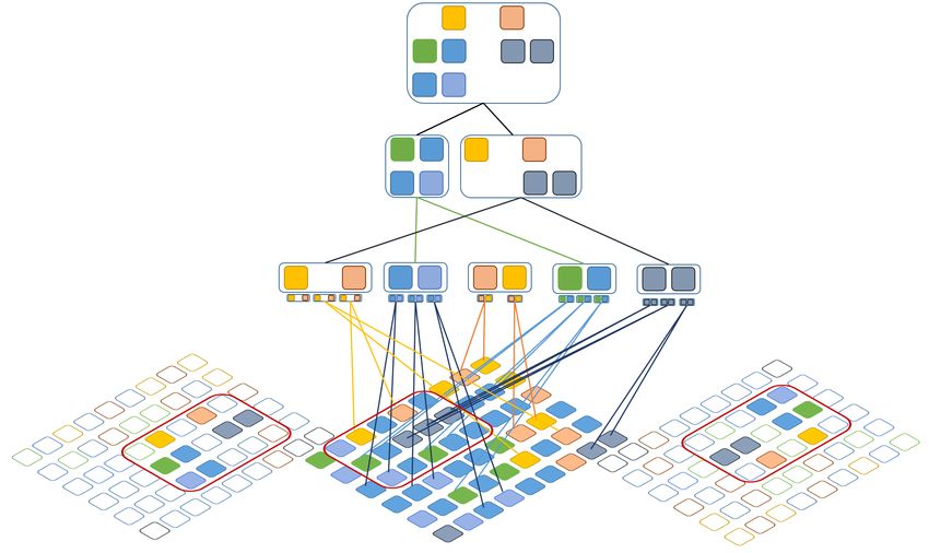
hierarchical model is shown in Figure 1.
The RhythmCHM model extracts a hierarchy of rhythmic patterns from its input. It is based on
relative encoding of time in rhythmic structures, which is commonly used in rhythmic representations
and is a necessity, as an individual rhythmic pattern may vary in duration due to tempo changes
within a music piece or due to different tempi across pieces in a music corpus. The model also contains
mechanisms that handle the variability of rhythmic patterns, which commonly occur during transitions
between segments (e.g., drum transitions) and in segment repetitions (e.g., half-feel and double-feel).
The structure of the model is illustrated in Figure 2. In the following subsections, we present the
model’s features and implementation.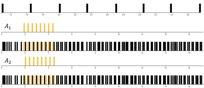
Appl. Sci. 2020, 10, 178                                                                                         5 of 22

      Figure 1. An abstract representation of the compositional hierarchical model. A composition of
      a complex structure in the input is marked in red. Each layer includes a set of parts which are
      compositions of parts from the previous layer. The structure may vary in its exact structure and position
      in the input. Part activations are depicted underneath each part on the first layer of compositions and
      represent occurrences of concepts in the input. Due to the relative encoding of parts, a part may activate
      at different locations within the input music signal. The entire structure of the model is transparent
      and allows for detailed analysis of the learned abstractions.

      Figure 2. An abstract representation of a learned rhythmic hierarchy. Each layer consists of a set
      of parts which are compositions of parts from the previous layer. For each part, we display the
      rhythmic pattern it encodes, while the connections between parts show how compositions are formed.
      The compositions are formed of (sub)parts, where the second subpart is encoded relatively to the first
      part in the composition. The part on the first layer P10 represents any occurrence of two input events.
      As the encoding of parts is time-invariant, parts activate wherever the patterns they encode occur in the
      input, regardless of their scaling. To illustrate this, we show three activations of the part P11 with three
      different time scales in the input. Altogether, only five L1 activations are shown, others are omitted
      for clarity.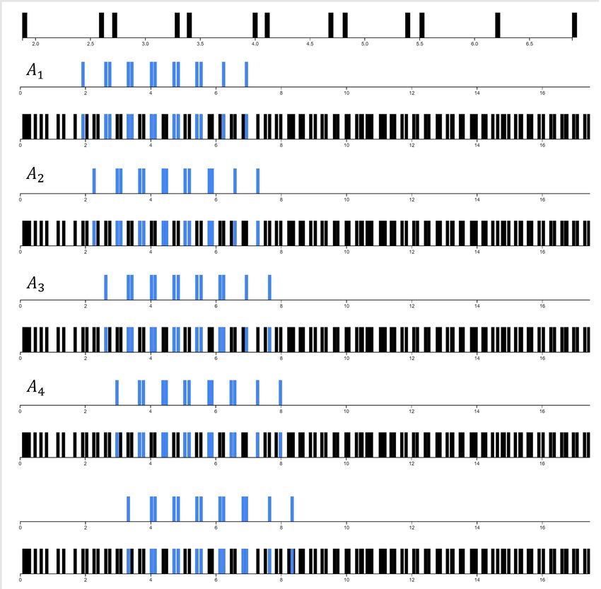
Appl. Sci. 2020, 10, 178                                                                                   6 of 22

2.1. Model Description
     The input of the RhythmCHM model consists of onset times and magnitudes of music events.
Pitches and note durations are ignored. Onsets may be extracted either from audio recordings (using
an onset detector) or from symbolic representations. Formally, the input can be described as a set of
onset time and magnitude tuples:

                                               I : {X : X = [ No , Nm ]}.                                     (1)

      The first layer of the model, denoted L0 , consists of a single atomic part P10 , where the superscript
is defined by the layer and the subscript marks the part number. Since any rhythm is composed of at
least two events (i.e., a single event cannot solely represent a rhythmic pattern), the part P10 represents
any occurrence of two events (onsets) in the input signal. The relation between the two events is
encoded in the part’s activation, which is calculated when an input sequence is presented to the model.
      The activation A represents any occurrence of a part P in the input and is composed of three
elements: the onset time A T is the onset time of the first event, the magnitude A M is the activation
magnitude, while the activation scale AS represents the scale of activation on the time axis. On the first
layer, AS is defined as the difference of onset times of both events. Namely, as each part, corresponding
to a rhythmic pattern in our model is relatively encoded, the activation scale represents the timing
(tempo/duration) with which the pattern has been located in the model’s input. The scale distinguishes
between two pattern occurrences found at the same onset, one faster (small scale), and one slower
(large scale). The activation magnitude A M represents the sum of event magnitudes. On the first layer,
the magnitude represents the onsets’ magnitudes Nm , as described in Equation (1). The magnitude is
therefore always non-negative; however, it can be diminished or inhibited (i.e., zero value) due to the
hallucination and inhibition mechanisms described later on in this Section.
      More formally, the part P10 activates for all pairs of input events i1 = [ No1 , Nm
                                                                                        1 ] and i = [ N 2 , N 2 ],
                                                                                                 2     o     m
where i1 occurs before i2 , as:

                           A = h A T , AS , A M i ← h No1 , No2 − No1 , ( Nm
                                                                           2
                                                                             + Nm1 )/2.i                      (2)

2.1.1. Rhythmic Compositions
     Each part on a successive layer Ln is a composition of one or more (sub-)parts on the previous
layer Ln−1 . Formally, a composition Pin of K subparts { Pkn−1 . . . Pkn−1 } is defined as:
                                                                         0          K −1

                               Pin = { Pkn−1 , { Pkn−1 , (µ1,j , σ1,j ), (µ2,j , σ2,j )}Kj=−11 }              (3)
                                           0         j

      Relations between the subparts forming the composition are governed by two Gaussians, which
control their relative spacing and scaling, leading to a tempo invariant representation of a rhythmic
pattern. All subparts relate to the first subpart of the composition.
      The first Gaussian with parameters (µ1,j , σ1,j ) defines the size of the subpart relative to the size
of the first subpart. Values of µ1 larger than one indicate that the second subpart is longer than the
first subpart; the values smaller than one indicate the inverse. When the model is trained on a corpus,
the values of µ1,j usually converge to integer ratios commonly present in different time signatures,
e.g., 1/5, 1/4, 1/3, 1/2, 1, 2, etc. Given activations subparts Pkn−1 and Pkn−1 , the value of µ1,1 is
                                                                             0     1
calculated as:
                                            AS ( Pkn−1 ) ∗ (1 + µ1 ( Pkn−1 ))
                                                    1                   1
                                   µ1,1 =                                     .                          (4)
                                            AS ( Pkn−1 ) ∗ (1 + µ1 ( Pkn−1 ))
                                                         0                      0

    The second Gaussian with parameters (µ2,j , σ2,j ) defines the placement (onset) of the second
subpart relative to the size of the first subpart. Thus, values larger than one indicate that the second
subpart’s onset comes after the end of the first subpart (there is a gap in between), the value of one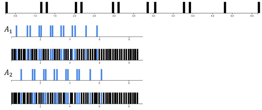
Appl. Sci. 2020, 10, 178                                                                                            7 of 22

means that the second subpart starts exactly at the end of the first subpart, while smaller values indicate
overlap between both subparts. The parameter µ2 is calculated from activations of two subparts as:

                                                   A T ( Pkn−1 ) − A T ( Pkn−1 )
                                                            1              0
                                        µ2,1 =                                       .                                  (5)
                                                 AS ( Pkn−1 ) ∗ (1 + µ1 ( Pkn−1 ))
                                                        0                      0

       The parameter σ1,1 is estimated from the distribution of pairs of activations with values near
µ1,1 , between 0.75–1.5 times the first subpart activation scale. Similarly, σ2,1 is estimated from the
distributions of pairs of activations with values near µ2,1 , within 0.75–1.5 of the first subpart’s length,
therefore [0.75*µ2,1 , 1.5*µ2,1 ]. These limits are imposed to exclude the influence of combinations of parts
which could represent a double or half beat granulation, and would significantly skew the Gaussian.
       In Figure 3, we show four simple first layer compositions with different values of µ1,1 and
µ2,1 . All parameters of a composition are learned during training and their values reflect the nature
of the training data. For example, in studio-recorded music, tempo will be more even, so the
variance of pattern lengths and their relative positions will be small, while the values will increase for
live recordings.

      Figure 3. An example of four different RhythmCHM compositions. In the first example, the second
      subpart is the same length as the first subpart and is positioned exactly one P10 length after the first
      subpart’s position. In P21 , the second subpart is the same length as the first subpart and occurs at twice
      its length. In P31 , the second subpart is twice the length of the first subpart and starts at half its length.
      In P41 , the second subpart is half the length of the first subpart and starts exactly at its end. The green
      arrow represents the length (1) of the first subpart, while the blue arrow represents the length of the
      second subpart. The offset of the second subpart is marked with a gray arrow.
Appl. Sci. 2020, 10, 178                                                                                 8 of 22

2.1.2. Activations of Parts on Higher Layers
     Activations of parts indicate the presence of the patterns they encode in the model’s input.
As already described, an activation has three components: time, which defines the starting time of
the pattern; scale, which establishes the length of the (relatively encoded) pattern and magnitude,
representing the activation’s strength. A part can activate only if all of its subparts are activated with
magnitude greater than zero (this constraint can be relaxed by the hallucination mechanism described
later on). Due to the relative encoding of patterns in the model, a part can have many simultaneous
activations (at different times and scales), indicating that the pattern it encodes has been found at
several locations in the input signal.
     An example is illustrated in Figure 4, which shows a simple L1 part with several activations at
the same time but on different scales. Note that the part’s encoding of a rhythmic pattern is relative
and its scale is only established during inference on a concrete music piece. Thus, the model’s parts
encode rhythmic information independently of tempo, and in this way the model may easily follow
patterns in pieces with changing tempo or in corpora that contain pieces in different tempi.

      Figure 4. An L1 part with three events is activated on a simple input signal. Four activations are
      shown, all occurring at the same time, but with different scales encoded in AS (between 0.25 and 1).

2.2. Learning and Inference
      The model is constructed layer-by-layer with unsupervised learning on a set of training examples,
starting with L1 . The learning process can be observed as a set-cover optimization problem, where we
aim to find a minimal set of compositions for the learned layer, which would (through their activations)
explain the maximal amount of information (events) present in the input data. The learning process is
driven by statistics of part activations, which captures regularities in the input data.

2.2.1. The Learning Algorithm
     We use a greedy approach to solve the set-cover problem. Learning takes place iteratively, where
in each iteration, we pick a composition which covers the largest amount of uncovered events in the
input and add it to the current layer. The learning algorithm is composed of two steps: finding a set of
candidate compositions and adding compositions to the layer.
     To construct the set of candidate compositions for a new layer Ln , we first calculate activations
of all parts from the layer L0 up to the layer Ln−1 . We then observe the co-occurrences of Ln−1
part activations on the training set within a time window. The co-occurrences indicate parts, which
frequently activate simultaneously in a certain relationship and are therefore candidates for forming
compositions, as they are assumed to form common concepts. They are estimated from histograms
of co-occurring part activations, which are formed according to the distances and scales of activation
pairs. New candidate compositions are formed from parts where the number of co-occurrences
Appl. Sci. 2020, 10, 178                                                                                   9 of 22

exceeds the learning threshold τL . The composition parameters µ1 , µ2 and σ1 , σ2 are estimated from
the corresponding histograms (an example is given in Figure 5) and each new composition is added to
the set of candidate compositions C . The pseudo-code of the procedure is shown in Figure 6.

       Figure 5. An example of the activation co-occurrence histogram. The axes represent the relative scale
       and locations of activations of a pair of parts.

 1: procedure CANDIDATECOMPOSITIONS(Ln )
 2: C = {}
 3: for (P1 , P2 ) ∈ Ln−1 × Ln−1 do

 4:     hist ← array(maxSize)
 5:     for Act1 ∈ P1 do
 6:        for Act2 ∈ P2 do
 7:           if withinWindow( Act1 , Act2 ) then
 8:           loc ← Act2 [ A T ] − Act1 [ A T ]
 9:           scale ← Act2 [ AS ]/Act1 [ AS ]
10:           hist[loc, scale] ← hist[loc, scale] + Act1 [ A M ] + Act2 [ A M ]
11:         end if
12:       end for
13:     end for
14:     peak ← peakPick(hist, τL )
15:     while peak 6= ∅ do
16:       [µ, σ] ← estimateGaussian(hist, peak);
17:       C ← C ∪ newPart( P1 , P2 , µ1 , σ1 , µ2 , σ2 )
18:       hist ← removeFromHist(hist, peak, µ, σ )
19:        peak ← peakPick(hist, τL )
20:     end while
21:   end for
22:   return C
                   Figure 6. The algorithm for generating histograms and candidate compositions.

     From the set of candidate compositions C , parts are iteratively chosen and added to the new layer
as follows:
Appl. Sci. 2020, 10, 178 10 of 22
• coverage of each part (events that part activations explain in the training set) is calculated,
• the part that adds most to the coverage of the entire training set is chosen. This ensures that only
compositions that provide enough coverage of “new” data with regard to the currently selected
set of parts will be added,
• the algorithm stops when the added coverage falls below the learning threshold τC or the overall
coverage reaches the threshold τP .
To avoid generating combinations, of which subpart activations are far apart, we limited the
search with the withinWindow( Act1 , Act2 ) function. The pseudo-code for selecting the candidate
compositions is outlined in Figure 7. Although the algorithm, which performs a greedy selection
of compositions, does not provide the optimal subset of part candidates, its output is sufficient for
the use in our model. The problem of candidate selection can be translated to a set-cover problem,
which is known to be NP-hard. The greedy approach therefore represents an approximation of the
best solution.
1: procedure SELECTCOMPOSITIONS(C )
2: prevCov ← 0
3: cov ← ∅
4: Ln ← ∅
5: sumInput ← |I|
6: repeat
7: for P ∈ C do
8: c←0
9: F ← coverage(Ln ∪ P)
10: c ← c + |F |
11: cov[ P] ← c/sumInput
12: end for
13: Chosen ← argmax(cov)
P
14: Ln ← Ln ∪ Chosen
15: C ← C \ Chosen
16: if cov[Chosen] − prevCov < τC then
17: break
18: end if
19: prevCov ← cov[Chosen]
20: until prevCov > τP ∨ C = ∅
21: return Ln
Figure 7. The greedy algorithm for selection of compositions from the candidate set C . Compositions
that add the most to the coverage of information in the learning set are prioritized.
The learning algorithm is repeated for each layer until a desired number of layers is reached.
The desired number of layers is dependent on the complexity of the input and the specificity of
the task. Simple rhythms can be observed on the first few layers, while higher layers contain more
complex rhythmic structures that can be used for differentiating between different rhythms on a
section-size level.
2.2.2. Inference
When a trained model is presented with new input data, the learned rhythmic patterns may be
located in the input through the process of inference. Inference calculates part activations on the input
data, bottom-up layer-by-layer, whereby the input data activates the layer L0 . For each occurrence ofAppl. Sci. 2020, 10, 178 11 of 22
a rhythmic pattern (part activation), the scaling factor, encoded in AS , determines the length of the
pattern, A T determines its onset time and A M its magnitude.
Inference may be exact or approximate. In the latter case, two mechanisms, hallucination and
inhibition can be used to tolerate for rhythmic irregularities in music.
In exact inference, a part is activated only if all of its subparts are activated. Hallucination relaxes
this condition and enables the model to produce activations even in the case of incomplete (missing,
masked or damaged) input. The model generates activations of parts, which most fittingly cover the
information present in the input signal, where fragments, which are not present, are hallucinated.
The missing information is therefore extrapolated from the knowledge acquired during learning,
encoded into the model structure. The amount of hallucination is governed by a threshold τH .
Inhibition performs hypothesis refinement by reducing the number of part activations on
individual layers. It provides a balancing factor in the model by reducing redundant activations.
Although the learning algorithm penalizes parts redundantly covering the input signal, some
redundant parts are retained. During inference, each layer may, therefore, produce multiple redundant
activations covering the same information in the input signal. Inhibition removes activations of parts
that have already been covered by stronger activations of other parts. The amount of removal can be
controlled by the inhibition threshold τI .
Approximate inference aids to the model’s ability to find rhythmic patterns with deletions, changes
or insertions, thus increasing its robustness. The inhibition mechanism has a more pronounced role in
the rhythmic model, because of the relativity of the encoded patterns and, typically, high regularity
of the input signal. Especially on the lower layers, a high number of activations representing simple
straight rhythmic patterns emerges, typically out of a few simple parts activating at different scales
and onsets. An example is given in Figure 8, which shows a series of activations of a simple L1 part on
a regular input signal. For clarity, only two different scales are shown in this example.
Figure 8. The example shows overlapping activations of a single P11 part. Inhibition can be employed
to efficiently reduce such overlapping activations.Appl. Sci. 2020, 10, 178 12 of 22
3. Analyses
We demonstrate the usability of the RhythmCHM model for extraction of rhythmic patterns in
two experiments. In the first, we assess how the model can extract patterns from different dance music
genres and how the extracted patterns characterize different genres. In the second, we show how the
model can extract patterns from individual music pieces, in which rhythm changes due to changing
time signatures, as well as tempo variations.
In both experiments, we extract rhythmic patterns from audio recordings. To detect the onsets
of music events in audio, we use the CNN onset detector [28]. As the onset detector does not output
onset magnitudes, we set all the magnitudes to the same value of one.
3.1. Experiment 1: Analyzing Ballroom Dances
We first evaluated the model’s ability to extract rhythmic patterns from music corpora. For the
purpose, we used the Ballroom dataset that is also used in many MIREX tasks (tempo and genre
estimation, beat tracking). The Ballroom dataset [7] is publicly available online (http://mtg.upf.edu/
ismir2004/contest/tempoContest/node5.html).
There are eight different genres in the Ballroom dataset—jive, rumba, cha cha, quickstep, samba,
tango, Viennese waltz, and (English) waltz. We trained our model on all pieces for a subset of genres
for which we expected to find distinctive rhythmic structures. For example, we expected to find swing
patterns in jive and similar patterns in rumba and cha cha but in different tempi. In the following
subsections, we report on the learned structures.
3.1.1. Jive
Jive music is based on a distinct swing rhythm, which contains unevenly spaced stressed events.
In its everyday occurrence on radios, the swing rhythm is commonly associated with jazz. Jive is a
medium to fast swing (commonly denoted as “uptempo”) and usually contains a happy or goofy tune.
Compared to other genres in the Ballroom dataset, jive is the only genre based on the swing rhythm.
In the model trained on all jive pieces in the dataset, we expected to observe distinct swing-like
rhythmic structures. The learned model contained 38 parts on five layers (number of parts per layer:
{2, 8, 10, 9, 9}). The analysis of the model revealed several compositions on different layers which
contained the distinct swing rhythmic structure.
An example of such a structure on the fifth layer is given in Figure 9. More interestingly, as shown
in Figure 10, the L5 part was generated from a single L4 part, the latter from a single L3 part and so on
to the first layer. The first layer contains only two parts, where the first part P11 represents three evenly
separated events (straight rhythm), with µ1 = 1, µ2 = 1 and the second subpart P21 an uneven rhythm
with µ1 = 0.86, µ2 = 1. This part composes all the parts with swing rhythm structures on the higher
layers L2 . . . L5 .
Along with these structures, the model also learned parts representing the basic straight rhythm.
The analysis of their activations showed that these parts activate on the downbeats of the rhythm,
interpreting the input as a straight meter and ignoring the syncopated second beat. In addition, such
parts also activated on the syncopated beats. This second group of activations, therefore, acted as
straight meter with shifted phase. An example is given in Figure 11.Appl. Sci. 2020, 10, 178 13 of 22
Figure 9. The L5 part representing the basic swing rhythm commonly found in jive songs. Below the
part’s structure, the first four activations are depicted individually with their projections onto the input
layer. The decomposition of the part’s structure is shown in Figure 10.
Figure 10. The structure of part P56 . All subpart compositions were formed from two instances of a
single part on layers {L0 . . . L5 }. The compositions’ parameters are shown on the right side. Each part
is shown twice with the offset used in the consecutive layer’s composition.Appl. Sci. 2020, 10, 178 14 of 22
Figure 11. The L5 part representing a straight rhythm. Below the part’s structure, two typical
activations are depicted individually with their projections onto the input layer. The first activation
covers eight consecutive downbeats, whereas the second activation covers the syncopation of the swing
rhythm in the input, imitating straight rhythm with shifted phase.
3.1.2. Samba
Samba’s rhythm partially resembles jive, with a distinctive difference in the timing of the second
beat, which is played in straight rhythm. Due to its syncopation of the second beat, we can expect
distinctive structures in the learned model, which cover the specific offset of the second beat in
the rhythmic pattern. As shown in Figure 12, the model trained on samba songs from the dataset
successfully captured the samba’s basic beat structure. The structure itself may seem similar to jive;
however, it differs in the ratio between the first and second beat. Compared to jive, the difference in
ratios is about 15 percent.
Figure 12. The L5 part representing the rhythmic pattern of a samba song. Below the part’s structure,
the first two activations are depicted individually with their projections onto the input layer. The part’s
structure is similar to jive, but contains different ratios between the first and the second beat.
3.1.3. Rumba and Cha Cha
Both music genres belong to the group of Latin-American dances. While the rumba dance and
music are associated with sensual topics, the cha cha contains more bright, powerful and uptempo
beats. Both music genres contain a distinctive “four-and-one” syncopation, which also defines the
basic steps in the dance. Additionally, both genres are played in straight meter with strong accents on
all four beats.Appl. Sci. 2020, 10, 178 15 of 22
We built a separate model for each genre and analyzed the learned structures. In contrast to
the previously analyzed genres, these two models shared a greater deal of straight rhythmic parts.
The rumba-trained model had 36 parts on five layers, while the cha-cha-trained model contained
33 parts.
Straight patterns dominated in both models. The distinctive patterns, containing the
“four-and-one” beats, were not as dominant as we initially expected. This was mainly the effect
of the variety of percussive and brass instruments playing granulated rhythmic riffs on and between
all beats, which the onset detector does not distinguish from the others. Therefore, straight patterns
dominate. The most closely associated typical pattern that was found is depicted in Figure 13.
Figure 13. The most prototypical part found in the cha cha trained model on layer L3 .
The “four-and-one” pattern is partially explained. However, two other eight-note events are
also included.
3.1.4. Tango
Although tango possesses South American roots, the widely known international (European)
version of the dance contains several aspects influenced by the European culture, such as the closed
position of the dancers, more common in standard dances. The music associated with this dance is
usually orchestral, played with severe stress on the syncopation (usually played by the violin and
other string instruments) on the offbeat before the downbeat.
In the trained model, we observed several parts forming a structure similar to the one displayed
in Figure 14. The off-beat is usually located between two beats and creates a syncopated rhythm,
for example, the first and the second beat in the meter, and can also appear on other locations. Onsets
of these beats have a fast attack and decay and usually a higher magnitude. The beat after is usually
omitted to create a deeper sensation of the stressed beats. Even though these properties are not
reflected in the input, which only contains the onset times, the learned structures do reflect the specifics
of the rhythm.
Figure 14. A tango part representing the regular “1-2-3-4” beats that match the meter and a syncopated
off-beat (third onset from the left).
3.2. Experiment 2: Robustness of the Model to Timing and Tempo Variations
The compositional structures in the model encode individual rhythmic patterns in a relative
representation. Such relative encoding makes the learned patterns independent of the underlying
tempo and minimizes the amount of parts per layer. During inference, activations of these
structures map them into absolute temporal space by scaling, where the scaling factor is encoded in
the activations.
To demonstrate the model’s ability to learn patterns regardless of the underlying tempo and its
ability to encode tempo changes in the scaling factor of each activation, we learned a model on a
Sirtaki song (Song available on Youtube: https://youtu.be/CbmbSjeUrxc, alternative version available
here: https://www.youtube.com/watch?v=dzlcxN0lxSo), which is well known for its rhythmic and
tempo changes.Appl. Sci. 2020, 10, 178 16 of 22
Due to the relative encoding of patterns, the entire hierarchy contains few parts on its five
layers—{2, 3, 7, 8, 8}. We show that by observing the scaling factor of part activations, we can infer
tempo changes in the analyzed song. More specifically, we focus on the segment (60–150 s) during
which the rhythm remains similar, but the tempo increases drastically. The segment starts with a
tempo of about 90 beats per minute and gradually increases up to 210 beats per minute. In Figure 15
we show how the scale of activations of a L6 part, representing ten straight beats, changes. The scaling
factor starts at 0.7 and decreases down to about 0.3. The ratio between the initial and the final scale
corresponds to the ratio between the initial and final tempo.
Figure 15. Scaling factor changes in the Sirtaki example as a consequence of tempo changes. The tempo
changes from roughly 90 to 210 beats per minute, causing the scale of part on layer L6 to change from
0.7 to 0.3.
To show the model’s ability to robustly extract rhythmic patterns in different time signatures from
a single music piece, we looked at live music recordings on Youtube. In this context, an interesting live
recording was produced by the Croatian singer Severina in a song “Djevojka sa sela” (Song available
on Youtube https://youtu.be/heJQAckM-eI). The live version performed at her concert in 2009 was
accompanied by trumpeters who played a 7/8 meter in verse, whereas the rock band played a 4/4
meter in the refrain. By training the model on this song, we produced a 5 layer hierarchy, containing
{3, 11, 11, 10, 9} parts on layers {L1 . . . L5 }, respectively. We first observed the three parts forming the
first layer. The part structures are depicted in Figure 16.
As is evident in Figure 16, two parts P11 and P31 activate across the entire song, while one part
activates only on the segments played in 7/8 meter. On layer L2 , we can find five parts which cover
5–6 rhythmic events, explaining the 7/8 segments—as the 7/8 meter can be broken into 3/8 + 2/8
+ 2/8 structure, these parts successfully find the downbeats of all three submeters. The remaining
six parts are the compositions of L1 parts, which cover both meters. Unfortunately, these parts also
compose the majority of L3 parts and further. This is a consequence of the statistical nature of the
model’s learning. Namely, the parts covering both meters cover a greater portion of the events when
compared to the parts covering only the 7/8 meter segments. Therefore, the greedy learning procedure
favours such parts on the higher layers and tends to ignore the 7/8-meter candidates with smaller
coverage. Nevertheless, the model successfully shows the ability to distinguish rhythmic structures
with different meters on L1 and L2 layers.Appl. Sci. 2020, 10, 178 17 of 22
Moreover, we selected this particular song, as it has a very uneven tempo due to the live
performance and the style of trumpet playing. The variations are visible in Figure 17, which shows
variations in the scale factor of activations of a L2 part, implying large differences in the timing of the
events covered by this part. The relative encoding of the compositions enables the model to extract the
rhythmic structures robustly in such circumstances.
Figure 16. The three parts forming the L1 layer for the Severina’s song. All activations for the parts P11
and P21 are shown in violet and blue colors respectively. It may be clearly observed that the P21 part
covers the input song segments played in 7/8 meter, while P11 and P31 activate across both 7/8 and 4/4
meters segments.
Figure 17. Varying activation sizes for a layer 2 part which activates on the 7/8 meter segments.
The majority of activations is within 100 milliseconds of the average size of 1.52 seconds (about 6%
difference in tempo); however, many occurrences also range from about 25% slower up to 25% faster).
4. Scalability and Visualization
4.1. Scalability
The goal of the presented compositional model is to provide an automated tool for rhythm
analysis of individual songs or entire corpora. Thus, scalability also plays an important role in itsAppl. Sci. 2020, 10, 178 18 of 22
applicability. The users should be able to use the model on their computers and mobile devices without
specialized hardware and large amounts of working memory. In this section, we first assess the time
complexity of model training, which is the most time-consuming part of model usage.
In order to evaluate how the model scales with the amount of training data, we trained 11
five-layer models on datasets ranging from 400 to 350,000 events (onsets). The training dataset
consisted of files from the ballroom dataset, augmented with 30-second clips of songs in a variety of
popular music styles.
The results are shown in Table 1. The time needed to train a model grows linearly with the number
of events. Training of a five-layer compositional structure on a database of approx. 350,000 events
take 50 min on a single core CPU. The linear dependency is clearly visible in Figure 18. Although a
single CPU core was used in our experiments, the model implementation is parallelized in most stages:
during learning, the generation of histograms, as well as candidate picking are both parallelized.
The inference process is also parallelized, except for the inhibition mechanism.
Table 1. The table summarizes the time needed and the number of learned parts when learning a
five-layer model with a different number of input events. The left side of the table shows the number
of music files and events in the input, along with the time needed to train a five-layer hierarchy. On the
right side, the number of parts per individual layer, along with the sum of all parts in the hierarchy,
is displayed.
# of Files Time (s) Events L1 L2 L3 L4 L5 # of Parts
2 3.77 389 2 6 9 10 9 36
4 5.16 660 3 10 9 9 10 41
8 10.43 1175 5 10 9 9 10 43
16 9.16 2307 3 10 9 8 9 39
32 20.13 4754 3 9 9 8 8 37
64 86.98 11,097 4 9 10 8 9 40
128 171.00 22,892 4 9 9 8 8 38
256 382.47 45,229 4 10 9 9 9 41
512 704.29 86,118 4 10 10 8 8 40
1024 1587.78 171,585 4 10 10 9 9 42
2048 3092.72 347,863 4 10 10 10 10 44
Figure 18. The graph shows the time needed to train a model (in seconds) in relation to the number of
input events. The dependency is linear.Appl. Sci. 2020, 10, 178 19 of 22
The amount of parts per layer grows only slowly with larger training datasets. Due to the relative
encoding of the learned structures, even small datasets can already produce parts general enough to
cover a variety of input data. The first layer is always small (3–4 parts), while the number of parts on
higher layers remains approximately constant (8–10 parts). Next to relative encoding, this is also likely
due to the similar rhythmic structures found in the dataset—it mostly covers popular music genres.
Using a more varied training dataset (e.g., music with very different metric structure) would likely
increase the number of parts. The results of this experiment show the model’s usability for rhythmic
analysis of large music corpora.
4.2. Visualizing the Patterns
Due to its transparency, the model can be utilized for visualization and exploration of the learned
hierarchy of rhythmic patterns and their occurrences within training data, as well as in new and unseen
data, within individual songs, or entire corpora. For this purpose, we developed a web visualization
tool to bring the model closer to the interested researchers.
Our visualization enables simple one-click inspection of individual model parts and occurrences
of rhythmic patterns they encode. An example is shown in Figure 19. Each part (pattern) is displayed
in a different color. Its description provides information on the part’s structure, as well as the total
coverage and activation magnitudes on the input data. When a pattern is selected, its structure is also
visualized (a straight pattern of nine events is shown in the Figure). All pattern occurrences are shown
as a list, as well as projected onto the input set of events at the bottom of the visualization. Based
on their goal, users may select individual activations or observe all activations of a specific pattern.
The visualized activations and the input are visualized at the bottom of the interface. The web interface
is publicly accessible at http://rhychm.musiclab.si/.
Figure 19. The web-based visualization of a model, showing a straight pattern and its occurrences in
the input. Each part (assigned an individual color) is described by the composition of subparts and their
offsets µ1 , µ2 , with some additional information, such as coverage of the input signal, self-overlapping
of the activations and the amount of covered events in the input signal. Each individual part can
be inspected by visualizing its structure and its projected activations onto the input visualization.
The time-span (in seconds) of the projection can be narrowed to the segments of interest.Appl. Sci. 2020, 10, 178 20 of 22
5. Conclusions
We presented a novel compositional hierarchical model for rhythm analysis. Its features are
unsupervised learning of relative tempo-invariant rhythmic structures, transparency, which enables
inspection of the learned concepts, and robustness in learning and inference.
We applied the model to recordings in the Ballroom dataset to analyze whether genre-specific
rhythmic structures can be learned. A separate model was trained for each genre. Due to transparency,
the learned structures were clearly interpretable and their analysis showed that the model is capable
of extracting rhythmic structures specific to individual genres. Additionally, we showed on different
examples that the model can robustly learn and infer patterns in pieces with changing tempo and
timing variations, as well as extract patterns corresponding to different time signatures. The model can
be unsupervisedly trained on a single music piece or on a corpus. A model trained and inferred on a
dataset containing a single genre will produce more activations with higher magnitudes than a model
trained on one genre and inferred on a different genre. If the model is trained on multiple genres,
some part activations occur only on a subset of songs, which contain structures those activated parts
describe. Other parts, especially lower-layer parts, will activate on a majority of songs with common
basic structure. In this aspect, the proposed approach can be observed as a probabilistic model for
rhythmic pattern discovery and can be employed for intra- and inter-corpus analysis.
The results indicate that the model can unsupervisedly extract rhythmic patterns in a variety of
conditions, without incorporating any assumptions on the specific meters or tempos. The patterns
emerge as a consequence of statistical regularities in the signal, while their relative encoding makes
them invariant to tempo changes. Therefore, the model is useful for rhythm analysis in a variety
of musical genres and also for non-Western music with more varied rhythms. The experiment that
involved large tempo changes showed the model’s ability to adjust the relatively encoded structures to
the tempo of the input signal and scale their activations accordingly.
The model provides the basis for several research directions which we intend to pursue in the
future. On one side, we will focus on the applicability of the model to specific problems musicologists
and music theorists experience in their research while using existing analytical tools. The model can be
used as support for semi-automatic music analysis, and we plan to make it more suitable for individual
use cases by developing user interfaces for learning and inference, as well as better visualization and
representation of the learned structures. Moreover, the proposed rhythmic model could be used as
a feature extractor for machine learning supported analyses and classification. Such application of
the model was previously demonstrated with the symbolic version of the proposed model [26] for
tune family classification. In terms of rhythm classification, the parts can be observed as features and
their activations could be translated to the values of these features. By selecting a subset of layers in a
learned model, the desired granularity of the features could be adjusted.
In its current state, the model discovers rhythmic patterns on a simple onset notation. To improve
its performance in learning complex rhythms, we will extend the model with accent encoding in
part structures. Additionally, we will extend the model with pitch information, thus merging it
with the compositional hierarchical model SymCHM [25] used for pattern discovery in symbolic
music. While the SymCHM discovers repeating melodic patterns in data, it ignores the rhythmic
information. Ren et al. [29] analyzed the results of different approaches and features in the classification
of folk songs and discovered the significance of rhythm-related features for discovery. The combined
rhythmic/melodic model could potentially improve the results in melodic pattern discovery and
related tasks.
Author Contributions: Conceptualization, M.M. and A.L.; methodology, M.M. and M.P.; software, M.P. and
M.M.; validation, M.P. and M.M.; formal analysis, M.P.; investigation, M.M.; resources, M.M.; data curation, M.P.;
writing—original draft preparation, M.P.; writing—review and editing, M.M.; visualization, M.P.; supervision,
M.M. and A.L. All authors have read and agree to the published version of the manuscript.
Funding: This research received no external funding
Conflicts of Interest: The authors declare no conflict of interest.Appl. Sci. 2020, 10, 178 21 of 22
References
1. Brochard, R.; Abecasis, D.; Potter, D.; Ragot, R.; Drake, C. The “Ticktock” of Our Internal Clock: Direct
Brain Evidence of Subjective Accents in Isochronous Sequences. Psychol. Sci. 2003, 14, 362–366. [CrossRef]
[PubMed]
2. Hansen, N.C.; Sadakata, M.; Pearce, M. Nonlinear Changes in the Rhythm of European Art Music:
Quantitative Support for Historical Musicology. Music Percept. Interdiscip. J. 2016, 33, 414–431. [CrossRef]
3. Toussaint, G.T. The Geometry of Musical Rhythm; Chapman and Hall/CRC: Boca Raton, FL, USA, 2016;
doi:10.1201/b13751. [CrossRef]
4. Bello, J.P.; Rowe, R.; Guedes, C.; Toussaint, G. Five Perspectives on Musical Rhythm. J. New Music Res. 2015,
44, 1–2. [CrossRef]
5. Sachs, C. Rhythm and Tempo: An Introduction. Music. Q. 1952, 38, 384–398. [CrossRef]
6. Downie, J.S. The music information retrieval evaluation exchange (2005–2007): A window into music
information retrieval research. Acoust. Sci. Technol. 2008, 29, 247–255. [CrossRef]
7. Dixon, S.; Gouyon, F.; Widmer, G. Towards Characterisation of Music via Rhythmic Patterns. In Proceedings
of the International Conference on Music Information Retrieval (ISMIR), Barcelona, Spain, 10–14 October
2004; pp. 509–516.
8. Esparza, T.M.; Bello, J.P.; Humphrey, E.J. From Genre Classification to Rhythm Similarity: Computational
and Musicological Insights. J. New Music Res. 2015, 44, 39–57. [CrossRef]
9. Böck, S.; Krebs, F.; Widmer, G. Accurate Tempo Estimation Based on Recurrent Neural Networks and
Resonating Comb Filters. In Proceedings of the International Conference on Music Information Retrieval
(ISMIR), Málaga, Spain, 26–30 October 2015; pp. 625–631.
10. Bock, S. Submission to the MIREX 2018: BeatTracker. In Proceedings of the MIREX 2018, Paris, France,
23–27 September 2018; pp. 1–2.
11. Bock, S.; Krebs, F. Submission to the MIREX 2018: DBNBeatTracker. In Proceedings of the MIREX 2018,
Paris, France, 23–27 September 2018; pp. 1–2.
12. Krebs, F.; Böck, S.; Widmer, G. Rhythmic pattern modeling for beat and downbeat tracking in musical audio.
In Proceedings of the International Conference on Music Information Retrieval (ISMIR), Curitiba, Brazil, 4–8
November 2013; pp. 1–6.
13. Huron, D. Tone and Voice: A Derivation of the Rules of Voice-Leading from Perceptual Principles. Music
Percept. 2001, 19, 1–64. [CrossRef]
14. Huron, D.B. Sweet Anticipation: Music and the Psychology of Expectation; MIT Press: Cambridge, MA, USA,
2006; p. 462.
15. Abdallah, S.; Plumbley, M. Information dynamics: Patterns of expectation and surprise in the perception of
music. Connect. Sci. 2009, 21, 89–117. [CrossRef]
16. Sioros, G.; Davies, M.E.P.; Guedes, C. A generative model for the characterization of musical rhythms. J. New
Music Res. 2018, 47, 114–128. [CrossRef]
17. Foscarin, F.; Jacquemard, F.; Rigaux, P. Modeling and Learning Rhythm Structure. In Proceedings of the
Sound & Music Computing Conference, Málaga, Spain, 28–31 May 2019.
18. Simonetta, F.; Carnovalini, F.; Orio, N.; Rodà, A. Symbolic Music Similarity through a Graph-Based
Representation. In Proceedings of the Audio Mostly 2018 on Sound in Immersion and Emotion—AM’18,
Wrexham, UK, 12–14 September 2018; ACM Press: New York, NY, USA, 2018; pp. 1–7. [CrossRef]
19. Temperley, D. A Unified Probabilistic Model for Polyphonic Music Analysis. J. New Music Res. 2009, 38, 3–18.
[CrossRef]
20. Temperley, D. Modeling Common-Practice Rhythm. Music Percept. Interdiscip. J. 2010, 27, 355–376. [CrossRef]
21. Holzapfel, A. Relation Between Surface Rhythm and Rhythmic Modes in Turkish Makam Music. J. New
Music Res. 2015, 44, 25–38. [CrossRef]
22. London, J.; Polak, R.; Jacoby, N. Rhythm histograms and musical meter: A corpus study of Malian percussion
music. Psychon. Bull. Rev. 2017, 24, 474–480. [CrossRef] [PubMed]
23. Panteli, M.; Dixon, S. On the Evaluation of Rhythmic and Melodic Descriptors for Music Similarity.
In Proceedings of the International Conference on Music Information Retrieval (ISMIR), New York City, NY,
USA, 7–11 August 2016; pp. 468–474.You can also read


