An Integrated Graphic Modeling System for Three-Dimensional Hydrodynamic and Water Quality Simulation in Lakes - MDPI
←
→
Page content transcription
If your browser does not render page correctly, please read the page content below

International Journal of
           Geo-Information

Article
An Integrated Graphic Modeling System for
Three-Dimensional Hydrodynamic and
Water Quality Simulation in Lakes
Mutao Huang 1 and Yong Tian 2,3, *
 1    School of Hydropower Engineering & Information Engineering, Huazhong University of Science & Technology,
      Wuhan 430074, China; huangmutao@hust.edu.cn
 2    School of Environmental Science & Technology, Southern University of Science & Technology,
      Shenzhen 518055, China
 3    State Environmental Protection Key Laboratory of Integrated Surface Water-Groundwater Pollution Control,
      School of Environmental Science and Engineering, Southern University of Science & Technology,
      Shenzhen 518055, China
 *    Correspondence: tiany@sustc.edu.cn; Tel.: +86-755-8801-8016

 Received: 10 November 2018; Accepted: 7 January 2019; Published: 9 January 2019

 Abstract: Understanding the complex hydrodynamics and transport processes are of primary
 importance to alleviate and control the eutrophication problem in lakes. Numerical models are used
 to simulate these processes. However, it is often difficult to perform such a numerical modeling
 simulation for common users. This study presented an integrated graphic modeling system designed
 for three-dimensional hydrodynamic and water quality simulation in lakes. The system, called the Lake
 Modeling System (LMS), provides necessary functionalities streamlined for hydrodynamic modeling.
 The LMS provides a geographic information system (GIS)-based data processing framework to
 establish a model and provides capabilities for displaying model input and output information.
 The LMS also provides mapping and visualization tools to support the model development process.
 All of these features in a GIS-based framework makes the task of complex hydrodynamic and water
 quality modeling easier. The applicability of the LMS is demonstrated by a case study in Lake
 Donghu, which is a large urban lake in the middle reaches of the Yangtze River in China. The LMS
 was utilized to setup and calibrate a model for Lake Donghu. Then the model was used to study the
 effects of a water diversion project on the change in hydrodynamics and the water quality.

 Keywords: three-dimensional hydrodynamics; water quality; lake; geographic information system;
 GIS-model integration

1. Introduction
     Lakes are valuable natural resources for water supply, food, irrigation, transportation, recreation,
and hydropower. Due to near-lake development, lake ecosystems are being threatened by
anthropogenic impacts, including nutrient pollution, increasing populations and intensification of land
use. Eutrophication of water bodies, one of the most widespread environmental problems, is found
worldwide, from the Great Lakes of North America [1] to Lake Tai of China [2] and Lake Victoria
in Africa [3]. Understanding the complex hydrodynamics and transport processes are of primary
importance to alleviate and control the eutrophication problem in lakes.
     Hydrodynamics is highly variable among lakes due to the different geometries, surrounding
topographies, hydrological loadings, and meteorological conditions. Hydrodynamics and transport
processes in lakes are also inherently three-dimensional (3D), driven by interactions of wind, surface
thermodynamics, and topography. The numerical model has become one of the most powerful

ISPRS Int. J. Geo-Inf. 2019, 8, 18; doi:10.3390/ijgi8010018                         www.mdpi.com/journal/ijgi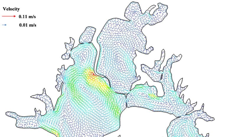
ISPRS Int. J. Geo-Inf. 2019, 8, 18                                                                2 of 22

tools for studying these complex dynamics. Such models can help us to know more clearly what
exactly is behind the water quality changes and eutrophication and help lake managers select optimal
control strategies. In past decades, many models and commercial software have been developed,
including Finite Volume Coastal Ocean Model (FVCOM) [4], Princeton Ocean Model (POM) [5],
Delft3D [6], Environmental Fluid Dynamics Code (EFDC) [7], and MIKE3 [8]. These models were
initially developed for ocean modeling; nevertheless they have been widely used to study a variety
of lake water issues, including lake water resources management [9], seasonal circulation, thermal
structure [10,11], and harmful algal blooms [12,13].
      Despite the fact that numerical models and scientific data sets are available for lakes’ numerical
modeling, great challenges remain for end users to conduct such modeling. On the one hand, a variety
of datasets are required to setup and calibrate a model, including bathymetry, meteorological data,
observations of hydrological variables (e.g., streamflow, water level, evaporation, etc.), water quality
variables (e.g., dissolved oxygen, chlorophyll, etc.), and many others. These data are usually large
in volume, multisource, multivariable, multidimensional, and heterogeneous, with complex spatial
and temporal regimes. Thus, incorporating all the data in the modeling process and interpreting
the results during decision making requires intensive data processing efforts and a comprehensive
understanding of the model. On the other hand, the setup of a numerical model involves many
steps, including computational grid generation, initial and open boundary condition settings, model
calibration, simulation and results analysis. It is often difficult to perform such a numerical modeling
simulation, even for a skilled user. These challenges have seriously hindered the wider application
of numerical models in scientific research and management practice. Therefore, a comprehensive
system that can handle the entire procedure of lake hydrodynamic and water quality modeling, from
data preparation at the very beginning to analysis and visualization of model outputs at the end, is
highly desired.
      It has been widely recognized that the Geographic Information System (GIS) plays a central
role in developing such a modeling system. Many efforts have been made to integrate the GIS
with numerical models for surface water (rivers, lakes, surface hydrology), coastal and ocean
modeling. For example, Liang et al. developed an automatic numerical simulation program for
coastal waters by integrating FVCOM with a GIS [14]; Ng et al. integrated a GIS with a complex
three-dimensional hydrodynamic sediment and heavy metal transport numerical model and applied
the integrated system to the Pearl River Estuary in China [15]; Qin and Lin developed a system for
costal seiches monitoring and forecasting by integrating FVCOM into a web-GIS based framework [16].
Such integrations not only benefit the preprocessing and postprocessing procedures of the modeling
but also provide the system with spatial data analysis and visualization capabilities. However, there
are several weaknesses associated with the existing systems, especially for lake modeling. First,
many GIS-hydrodynamic water quality models are two-dimensional. Since hydrodynamics in lakes
is intrinsically three-dimensional, such models may oversimplify the actual situations and produce
results with limited accuracy. Second, popular GIS platforms, such as ArcGIS Map and Google
Earth, are often used as the GIS environment by existing systems. However, these platforms are not
specifically designed for hydrodynamic studies and cannot easily handle the diversified data types
involved in the hydrodynamic modeling, especially time series data [17].
      In this paper, we present the design and development of the Lake Modeling System (LMS),
which is a modeling system for three-dimensional (3D) hydrodynamic and water quality model.
LMS provides graphic user interface (GUI) for end users to build 3D model. It provides a GIS-based
data processing framework for establishing the model and provides capabilities for displaying
and modifying model elements (model grids) and boundary conditions. The interface of LMS
is two-dimensional (2D) but allows to display and analyze model inputs and outputs that are
multi-dimensional. All of these features will make the task of hydrodynamic and water quality
modeling easier. The applicability of LMS is illustrated by a case study in Lake Donghu, which is a
large urban lake in the middle reaches of the Yangtze River.
ISPRS Int. J. Geo-Inf. 2019, 8, 18                                                                                           3 of 22

     In the remainder of this paper, Section 2 introduces the framework of the LMS, including the
system design and implementation. The details of setting up and running the model using the LMS
are also illustrated. Section 3 describes the application case of the LMS in the Lake Donghu in China.
The results and analysis of the Lake Donghu model are presented in Section 4, and conclusions are
provided in Section 5.

2. Framework of the System

2.1. Introduction to FVCOM-LAKE
    The current version of the LMS has been made compatible with the Finite Volume Coastal
Ocean Model (FVCOM) [4]. FVCOM appears to be one of the most popular modules for near
shore numerical simulation based on its prevalence in simulation literature [18,19]. It is an
unstructured-grid, finite-volume, three-dimensional (3-D) primitive equation ocean model with a
generalized, terrain-following coordinate system in the vertical and a triangular grid in the horizontal.
The unstructured grid can be designed to provide a customized variable resolution to both lake
boundaries and bathymetry.
    FVCOM uses the σ coordinate, which enables for a smooth representation of irregular bottom
topography to be obtained. The σ coordinate transformation is defined as:

                                                               z−ζ   z−ζ
                                                          σ=       =                                                            (1)
                                                               H+ζ    D

where H is the bottom depth (relative to z = 0) and ζ is the height of the free surface (relative to z = 0);
D = H + ζ is the total water column depth; and σ varies from −1 at the bottom to 0 at the surface.
In this coordinate, the governing equations of FVCOM consist of the following continuity, momentum,
temperature, salinity and density equations:

                                                      ∂ζ   ∂Hu ∂Hv ∂w
                                                         +     +    +    =0                                                     (2)
                                                      ∂t    ∂x   ∂y   ∂σ

           ∂Du       ∂Du2       ∂Duv      ∂uw
            ∂t   +    ∂x    +    ∂y    +   ∂σ
                                                      gD ∂       R0                                                           (3)
                                 =          ∂ξ
                                       − gD ∂x    −   ρ0 [ ∂x ( D σ   ρdσ0 ) + ρσ ∂D
                                                                                  ∂x ] +
                                                                                           1 ∂
                                                                                           D ∂σ
                                                                                                         ∂u
                                                                                                      Km ∂σ   + f vD + DFx

           ∂Dv       ∂Dv2       ∂Duv      ∂vw
            ∂t   +    ∂x    +    ∂y    +   ∂σ
                                                      gD ∂       R0                                                           (4)
                                 =           ∂ξ
                                       − gD ∂y    −   ρ0 [ ∂y ( D σ   ρdσ0 ) + ρσ ∂D
                                                                                  ∂y ] +
                                                                                           1 ∂
                                                                                           D ∂σ
                                                                                                         ∂v
                                                                                                      Km ∂σ   − f uD + DFy

                                 ∂DT   ∂DuT   ∂DvT   ∂wT   1 ∂    ∂T
                                     +      +      +     =     (K    ) + DFT                                                    (5)
                                  ∂t    ∂x     ∂y     ∂σ   D ∂σ h ∂σ
                                ∂DC ∂DuC ∂DvC ∂wC    1 ∂    ∂C
                                    +    +    +    =     (K    ) + DFC                                                          (6)
                                 ∂t   ∂x   ∂y   ∂σ   D ∂σ h ∂σ
                                                               ρ = ρ( T, C )                                                    (7)

where u, v, and w are the x, y, z velocity components, respectively; T is the temperature; C is the
salinity; ρ is the density; f is the Coriolis parameter; g is the gravitational acceleration; Km is
the vertical eddy viscosity coefficient; and Kh is the thermal vertical eddy diffusion coefficient.
Fx , Fy , FT , and FC represent the horizontal momentum, thermal, and salt diffusion terms, respectively.
Km and Kh are parameterized using the modified Mellor and Yamada level-2.5 (MY-2.5) turbulent
closure scheme [20–22]. FVCOM is numerically solved using a split-mode method.
      The water quality model used in this study is the Water Analysis Simulation Program (WASP) [23].
The conceptual model framework is shown in Figure 1. The model contains eight state variables,
including dissolved oxygen (DO; mg O2 L−1 ), carbonaceous biochemical oxygen demand (CBOD;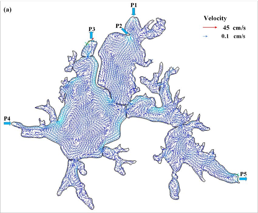
ISPRS Int. J. Geo-Inf. 2019, 8, 18 4 of 22
ISPRS Int. J. Geo-Inf. 2019, 8, x FOR PEER REVIEW 4 of 22
mg O2 L−1 ), nitrite nitrogen (NO3 ; mg N L−1 ), ammonium nitrogen (NH4 ; mg N L−1 ), organic nitrogen
(ON;O2mg L−1 ),nitrogen
L−1),Nnitrite organic (NO
phosphorus
3; mg N L−1(OP; mg P L−1nitrogen
), ammonium ), soluble(NH reactive
4; mg N phosphorus
L−1), organic(PO 4 ; mg P
nitrogen L−1 ),
(ON;
andmg N L−1), organic
phytoplankton phosphorus
biomass (OP; as
expressed mgchlorophyll
P L−1), soluble (CHL; reactive α L−1 ). The(PO
µg Chlphosphorus 4; mg P L
governing −1), and
equations
phytoplankton
of the biomass in
WASP are described expressed
detail inas chlorophyll
[24]. The WASP (CHL;
was μg Chl αwith
coupled L ). FVCOM
−1 The governing
and can equations
be run inofan
the WASP
online mode. are described
In this study,in
thedetail
suminof[24].
NH4The, NO WASP
3 , andwas
ON coupled
is with
regarded FVCOM
as the and
total can
nitrogenbe run in an
(TN), and
online mode. In this study, the sum of NH , NO
the sum of OP and PO4 is regarded as the total phosphorus (TP).
4 3 , and ON is regarded as the total nitrogen (TN), and
the sum
The of OP andenvironment
preferred PO4 is regardedforasbuilding
the total andphosphorus
running(TP). FVCOM is Linux. However, LMS is
designed to run on Windows. To this end, the source code ofFVCOM
The preferred environment for building and running FVCOMiswas Linux.
portedHowever, LMS is
to the Windows
designed to run on Windows. To this end, the source code of FVCOM
environment and was compiled as a standalone execution program using the Intel Fortran compiler.was ported to the Windows
environment and was compiled as a standalone execution program using the Intel Fortran compiler.
This modified version of FVCOM was called FVCOM-LAKE. The original algorithm of FVCOM has
This modified version of FVCOM was called FVCOM-LAKE. The original algorithm of FVCOM has
not been modified.
not been modified.
• Winds • Advection
• Heat flux FVCOM- • Dispersion • External loads
• Boundary fluxes LAKE • Temperature • Light
• River discharges • Salinity
Denitrification
Air-lake flux
Water Column
Nitrification
CBOD NH4 NO3 PO4
Uptake Uptake Uptake
Mineralization
Mineralization
Loss
Loss
Loss
Denitrification
Oxidation
Settling
Loss Loss
ON CHL OP
photosynthesis
Respiration
Benthic fluxes
Settling
Settling
Settling
DO
Sediment
Benthic oxygen
photosynthesis consumption
Sediment
Figure
Figure 1. 1.Conceptual
Conceptualframework
frameworkof
of the
the WASP
WASP water
water quality
qualitymodel.
model.
2.2.2.2. System
System Design
Design
Figure
Figure 2 presents
2 presents a conceptual
a conceptual design
design ofof
thethe GIS-modelintegration
GIS-model integrationframework.
framework.The Theframework
framework is
is composed of four major parts: the GIS-based user interface (UI), shared libraries,
composed of four major parts: the GIS-based user interface (UI), shared libraries, the three-dimensional the three-
dimensional hydrodynamic
hydrodynamic and water quality and water
modelquality model (i.e., FVCOM-LAKE)
(i.e., FVCOM-LAKE) and data The
and data sources. sources.
userThe user
interface
interface provides common GIS capabilities, such as mapping, management and analysis
provides common GIS capabilities, such as mapping, management and analysis of spatial information, of spatial
andinformation, and provides tools.
provides geo-processing geo-processing
The UI alsotools. The to
enables UIcreate
also enables
a modeltoand
create a model
perform andprocessing
model perform
model processing such as visualization of model inputs/outputs and animation of results. The data
such as visualization of model inputs/outputs and animation of results. The data and GIS libraries
and GIS libraries provides shared functions for reading, querying and manipulating data from the
provides shared functions for reading, querying and manipulating data from the underlying data
underlying data sources. The model wrapper provides functions that enable the system to
sources. The model wrapper provides functions that enable the system to communicate with the
communicate with the numerical model through input/output files. The actual execution of the
numerical model through input/output files. The actual execution of the numerical model is a
numerical model is a stand-alone program that does not require any GIS capabilities. The data
stand-alone program that does not require any GIS capabilities. The data sources include GIS data files
sources include GIS data files (i.e., raster and vector files), the relation database that stores time series,
(i.e.,and
raster andinput/output
model vector files),files.
the relation database that stores time series, and model input/output files.
ISPRS Int. J. Geo-Inf. 2019, 8, 18                                                                                  5 of 22
ISPRS Int. J. Geo-Inf. 2019, 8, x FOR PEER REVIEW                                                                  5 of 22

      Figure 2. Conceptual
      Figure 2. Conceptual diagram
                           diagram of
                                   of integration
                                      integration of
                                                  of aa GIS
                                                        GIS and
                                                            and aa three-dimensional
                                                                   three-dimensional hydrodynamic
                                                                                     hydrodynamic and
                                                                                                  and
      water quality model.
      water quality model.

2.3. System
2.3. System Implimentation
            Implimentation

2.3.1. System
2.3.1. System Overview
              Overview
      LMS was
      LMS    was developed
                  developed usingusing C#
                                        C# language
                                            language based
                                                         based onon Microsoft
                                                                     Microsoft .NET
                                                                                  .NET platform.
                                                                                          platform. TheThe DotSaptial
                                                                                                             DotSaptial
library [25] was employed for providing GIS environment. DotSpatial is a free and openopen
library  [25]  was  employed      for providing    GIS   environment.      DotSpatial    is a  free  and     sourcesource
                                                                                                                      GIS
GIS  library  written   for .NET.  It allows  developers    to incorporate    spatial   data, analysis
library written for .NET. It allows developers to incorporate spatial data, analysis and mapping         and    mapping
functionality into
functionality   into their
                      theirapplications.
                             applications.The
                                            Thegraphic
                                                 graphicuser   interface
                                                            user          of of
                                                                  interface  LMSLMS is shown
                                                                                       is shown in Figure
                                                                                                   in Figure3a. LMS    has
                                                                                                                 3a. LMS
a familiar  interface  similar  to most  desktop  GIS   applications.   The  main   window     contains
has a familiar interface similar to most desktop GIS applications. The main window contains a main        a  main   menu,
a map aviewer,
menu,             a legend,
           map viewer,         a toolbox
                            a legend,     and toolbars.
                                        a toolbox           The mapThe
                                                    and toolbars.       viewmapis the
                                                                                   viewmain   visualization
                                                                                          is the                 element.
                                                                                                   main visualization
LMS    provides   common      functionalities  to display    and   manage    geospatial    data,
element. LMS provides common functionalities to display and manage geospatial data, such as zoom, such   as  zoom,    pan,
query,query,
pan,    symbology,     conversion,
               symbology,             and many
                               conversion,   and other.
                                                  many The      toolbox
                                                           other.         also provides
                                                                   The toolbox              a set of atools
                                                                                   also provides        set to
                                                                                                             of perform
                                                                                                                 tools to
fundamental     GIS   operations.   LMS   supports    common      vector  and  raster   geospatial
perform fundamental GIS operations. LMS supports common vector and raster geospatial data            data   file formats.
                                                                                                                       file
The vector
formats.  Thedata  format
               vector   data supported    is shapefile,
                              format supported            and the
                                                  is shapefile,     raster
                                                                  and       data formats
                                                                       the raster            supported
                                                                                   data formats    supportedinclude    TIF,
                                                                                                                  include
PNG,PNG,
TIF,   JPEG,JPEG,
               and others.    LMS uses
                      and others.   LMSthe    project
                                           uses        to organize
                                                 the project         the model
                                                                to organize    theinformation     and otherand
                                                                                    model information          resources
                                                                                                                     other
resources required for the modeling. When opening a project, the model structure is presentedproject
required   for the modeling.      When   opening   a  project,  the  model   structure   is presented     in  the   in the
manager
project    (Figure (Figure
         manager    3b).      3b).
2.3.2. Grid Generation
2.3.2. Grid Generation
      LMS provides a grid generation tool to produce a high-quality triangular grid. This tool is based
      LMS provides a grid generation tool to produce a high-quality triangular grid. This tool is based
on the Delaunay triangulation algorithm developed by Shewchuk [26]. Figure 4 presents the grid
on the Delaunay triangulation algorithm developed by Shewchuk [26]. Figure 4 presents the grid
generation tool. The first step of using the tool is to specify a shapefile that represents a lake boundary.
generation tool. The first step of using the tool is to specify a shapefile that represents a lake boundary.
To improve the grid’s quality, the boundary line must be preprocessed, which includes smoothing and
To improve the grid’s quality, the boundary line must be preprocessed, which includes smoothing
redistributing the line’s vertices. The LMS provides a tool to perform these preprocessing operations.
and redistributing the line’s vertices. The LMS provides a tool to perform these preprocessing
The next step is to select a raster file that represents the lake’s bathymetry. Then, users can specify the
operations. The next step is to select a raster file that represents the lake’s bathymetry. Then, users
parameters that control the size and number of triangular elements and the method of interpolating
can specify the parameters that control the size and number of triangular elements and the method
the bathymetry. At this point, all requirements for the generation are satisfied, and the grid can be
of interpolating the bathymetry. At this point, all requirements for the generation are satisfied, and
automatically generated with the user’s click of a button. During the generation, bathymetry data will
the grid can be automatically generated with the user’s click of a button. During the generation,
be automatically interpolated to each node of the grid. LMS also accepts a grid file format generated
bathymetry data will be automatically interpolated to each node of the grid. LMS also accepts a grid
by other software, such as the Aquaveo Surface-water Modeling System.
file format generated by other software, such as the Aquaveo Surface-water Modeling System.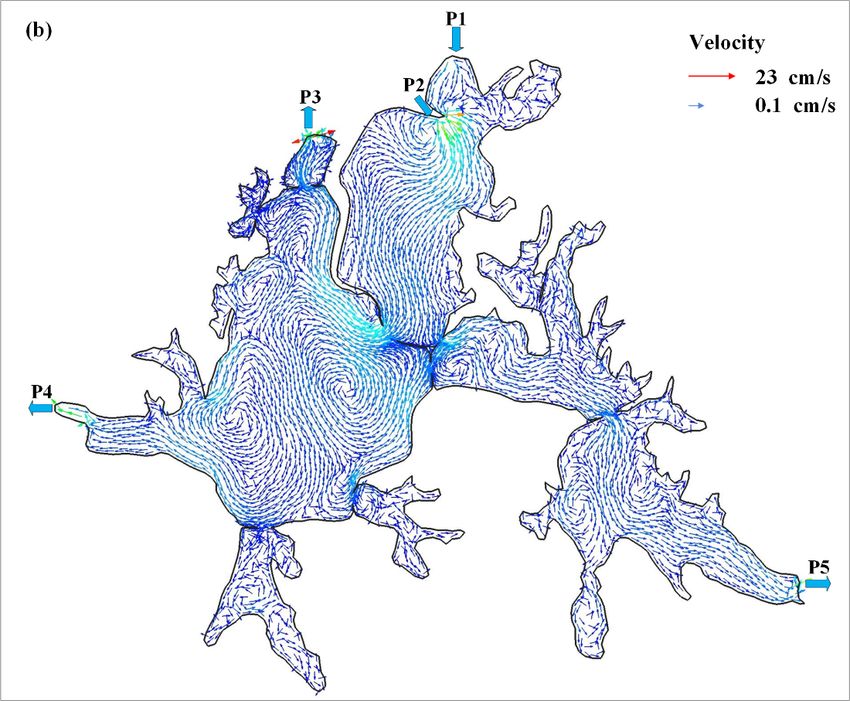
ISPRS Int. J. Geo-Inf. 2019, 8, 18                                                                       6 of 22

ISPRS Int. J. Geo-Inf. 2019, 8, x FOR PEER REVIEW                                                        6 of 22
 ISPRS Int. J. Geo-Inf. 2019, 8, x FOR PEER REVIEW                                                        6 of 22

              Figure 3. Main graphic user interface of LMS: (a) Map Viewer; and (b) Project Manager.
               Figure 3. Main graphic user interface
               Figure 3.                   interface of
                                                     of LMS:
                                                        LMS: (a)
                                                             (a) Map
                                                                 Map Viewer;
                                                                     Viewer; and
                                                                             and (b)
                                                                                  (b) Project
                                                                                      ProjectManager.
                                                                                              Manager.

                                            Figure 4. Grid generation tool.
                                             Figure4.
                                            Figure  4. Grid
                                                       Grid generation
                                                            generation tool.
                                                                        tool.
ISPRS Int. J. Geo-Inf. 2019, 8, 18 7 of 22
ISPRS Int. J. Geo-Inf. 2019, 8, x FOR PEER REVIEW 7 of 22
The generated
The generated grid
grid is
is represented
represented by by two
two shapefiles:
shapefiles: one
one is
is aa polygon
polygon shapefile
shapefile that
that represents
represents
the triangular elements of the grid, and the other is a point shapefile that represents the nodes
the triangular elements of the grid, and the other is a point shapefile that represents the nodes of of the
the
grid. These
grid. These two
two shapefiles
shapefiles will
will be
be added
added to
to the
the map
map view
view after
after the
the generation. The grid
generation. The grid input
input files
files
required by FVCOM-LAKE will also be generated.
required by FVCOM-LAKE will also be generated.
2.3.3. Initial and Boundary Conditions Settings
2.3.3. Initial and Boundary Conditions Settings
Users must define initial hydrodynamic values and initial quality state variables at each node
Users must define initial hydrodynamic values and initial quality state variables at each node of
of the grid. The state variables include the water level, water temperature and salinity, and the eight
the grid. The state variables include the water level, water temperature and salinity, and the eight
water column state variables. Ideally, the initial values should be determined based on observations.
water column state variables. Ideally, the initial values should be determined based on observations.
If such observations are unavailable, the initial values could be simply set as constants. If there are
If such observations are unavailable, the initial values could be simply set as constants. If there are
sufficient observations, the initial values could be assigned to the grid using several GIS tools provided
sufficient observations, the initial values could be assigned to the grid using several GIS tools
by LMS. For example, if observations are made on point stations, the Interpolation Tool could be used
provided by LMS. For example, if observations are made on point stations, the Interpolation Tool
to interpolate the observed point values to each node of the grid. Sometimes results generated by other
could be used to interpolate the observed point values to each node of the grid. Sometimes results
models or products produced by remote sensing methods (e.g., MODIS products) could also be used to
generated by other models or products produced by remote sensing methods (e.g., MODIS products)
set the initial values. These results or products are usually archived using the NetCDF format or other
could also be used to set the initial values. These results or products are usually archived using the
popular raster formats (e.g., TIF). The LMS enables initial conditions to be set by extracting the values
NetCDF format or other popular raster formats (e.g., TIF). The LMS enables initial conditions to be
from these data sets to the grid. Figure 5 presents the interface used to set the river boundary condition.
set by extracting the values from these data sets to the grid. Figure 5 presents the interface used to set
The user can specify nodes where river inflow/outflow would be applied, and set the discharge and
the river boundary condition. The user can specify nodes where river inflow/outflow would be
water temperature at the nodes.
applied, and set the discharge and water temperature at the nodes.
Figure 5. Interface used to set river boundary condition.
Figure 5. Interface used to set river boundary condition.
2.3.4. Driving
Driving Force
Force and Calibration Dataset Generation
FVCOM-LAKE
FVCOM-LAKE requires requires hourly
hourly meteorological
meteorological data as the driving force. force. The meteorological
variables include
includeprecipitation,
precipitation,air air pressure,
pressure, temperature,
temperature, wind and
wind speed speed and direction,
direction, relative
relative humidity,
humidity,
and sunshine andhours.
sunshineThehours. The heat-fluxes
heat-fluxes at the waterat the waterincluding
surface, surface, including
the sensibletheheat
sensible
flux, heat flux,
the latent
the
flux,latent flux, the incoming
the incoming longwavelongwave flux, the outgoing
flux, the outgoing longwave longwave
flux and flux and the incident
the incident short
short wave wave
flux are
flux are automatically
automatically calculatedcalculated
based onbased on the meteorological
the meteorological data. Thedata. The meteorological
meteorological data are
data are often often
archived
archived
in variousinformats,
varioussuch
formats, such as TXT,
as NetCDF, NetCDF, TXT, and
and Excel. LMS Excel. LMSaprovides
provides a set of conversion
set of conversion tools
tools to convert
to convert
these these
different different
formats intoformats
the inputinto
filethe input file
required required by FVCOM-LAKE.
by FVCOM-LAKE. The forces
The other driving other driving
include
forces include water
water discharge discharge and
and containment containment
concentration concentration
at rivers or drainage at facilities.
rivers or Observations
drainage facilities.
made
Observations madesuch
at sites or stations, at sites or stations,
as the water level,suchwater
as thetemperature
water level, and
water temperature
water and water quality
quality concentrations, are
concentrations, are usually
usually used to conduct used
model to conduct
calibration. model
The LMS calibration.
uses database Theto LMS
store uses
thesedatabase to store
observations. Thethese
user
observations.
can use ODM The user Manager
Database can use ODM
to import Database Manager
and manage to import datasets.
the calibration and manage the calibration
datasets.
ISPRS Int. J. Geo-Inf. 2019, 8, 18                                                                  8 of 22

2.3.5. Modeling Running and Postprocessing
      The users can start a model run once all necessary input files are ready. The running information
(e.g., simulation time, execution time, etc.) is synchronously displayed in a window. Any warnings or
errors information encountered during the modeling simulation will also be displayed in the window.
The users can stop the simulation at any time. The LMS allows the users to analyze the model outputs
at any time before the simulation is finished. When a model simulation takes long time to finish (e.g.,
hours or even days), this functionality is very useful since it allows the user to investigate problems or
errors and start a new simulation immediately.
      The output of the FVCOM-LAKE model consists of a set of binary files. The key output variables
include horizontal velocity magnitude and direction, vertical velocity magnitude, water level, and
concentration of water quality variables. With some simple operations, modeling results can be directly
loaded from the output files, processed and then displayed in the GIS environment. In LMS, each
model entity (e.g., grid, river inlet/outlets and boundaries) is represented by a FeatureSet object, which
is a general object in most existing GIS libraries. The FeatureSet object is used a shared data model
between GIS and the system. The loaded data is visualized through the FeatureSet object. In addition,
LMS provides several tools to display the modeling results in the form of time series, and profile.
      The profile tool extracts values at a selected point from each of the depth layers and then create
a profile plot using the extracted values. When using the profile tool, the user can click any point
within the modeling domain. The time series tool is used to display the time series of a selected
variable associated with a given point selected in a modeling domain. As the lake’s hydrodynamics
is continuously changing, the dynamic display of the modeling results is essential for examining
and analyzing spatiotemporal variations of the lake data. The LMS provides an animation tool that
enables the model outputs to be animated for the selected time span. Users are able to manipulate
the animation through a controller which provides common operations, including play, stop, pause,
forward, and backward. As the output data are loaded onto the computer memory, the system can
provide fluent animation. In addition, the system is able to perform basic data analyses (e.g., deriving
mean, sum, and maximum and minimum values) for user-specified time periods and spatial chart
view. This functionality is very useful in examining modeling results.

3. Case Study

3.1. Study Area
     An example is presented in this section to illustrate the use of the LMS for setting up a new model
run. Lake Donghu, a large urban lake, was selected as the case study area (Figure 6a). The lake is
fully located within the urban area of Wuhan city. It covers an area of 30.7 km2 and has an average
depth of 2.2 m. There are other five urban lakes around Lake Donghu, including Lakes Shahu, Beihu,
Yandonghu, and Yanxihu. Lake Donghu used to connect with Yangtze River. However, the lake was
completely separated from the Yangtze River in the 1980s and was divided into a set of bays by roads.
As presented in Figure 6b, the major bays include Tanglinhu, Shaojihu, Guozheng, Tuanhu, Miaohu,
Yujiahu, Yingwohu, and Shuiguo Bays.
     Lake Donghu is a typical shallow lake with limited contamination purification capabilities.
Pollutants are difficult to remove once they enter the lake. Before the 1950s, the lake was in good
health, and lake water could be used as drinking water. In the 1960s, the lake underwent oligotrophic
conditions, which gradually became mesotrophic by 1981. Since then, the situation has worsened due
to increasing contamination factors, such as increasing amounts of aquaculture, rapid urbanization,
and large quantities of wastewater discharged into the lake without proper treatment.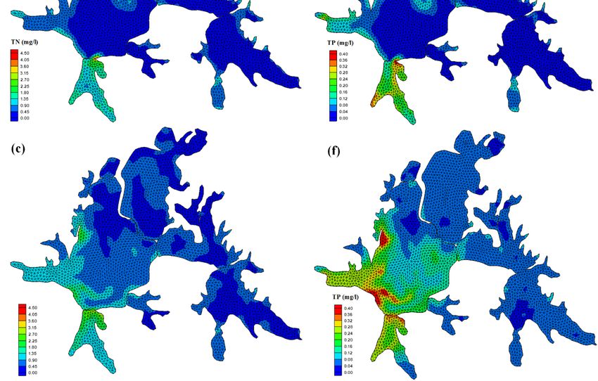
ISPRS Int. J. Geo-Inf. 2019, 8, 18                                                                       9 of 22
   ISPRS Int. J. Geo-Inf. 2019, 8, x FOR PEER REVIEW                                                  9 of 22

         Figure 6. The study area: (a) Lake Donghu and its surrounding urban lakes; and (b) water quality
      Figure 6. The study area: (a) Lake Donghu and its surrounding urban lakes; and (b) water quality in
         in Lake Donghu in May 2011.
      Lake Donghu in May 2011.

        Monthly samples of DO, nutrients and chlorophyll were collected at Stations W1 to W4 (Figure 6)
      Monthly samples of DO, nutrients and chlorophyll were collected at Stations W1 to W4 (Figure 6)
   by the Water Authority of Wuhan. Based on the measurements made in May 2011, the water quality
by the Water Authority of Wuhan. Based on the measurements made in May 2011, the water quality
   classification in the major bays of Lake Donghu was determined according to the Chinese national
classification in the major bays of Lake Donghu was determined according to the Chinese national
   water quality standard [27] and presented in Figure 6b. It can be seen that water qualities in most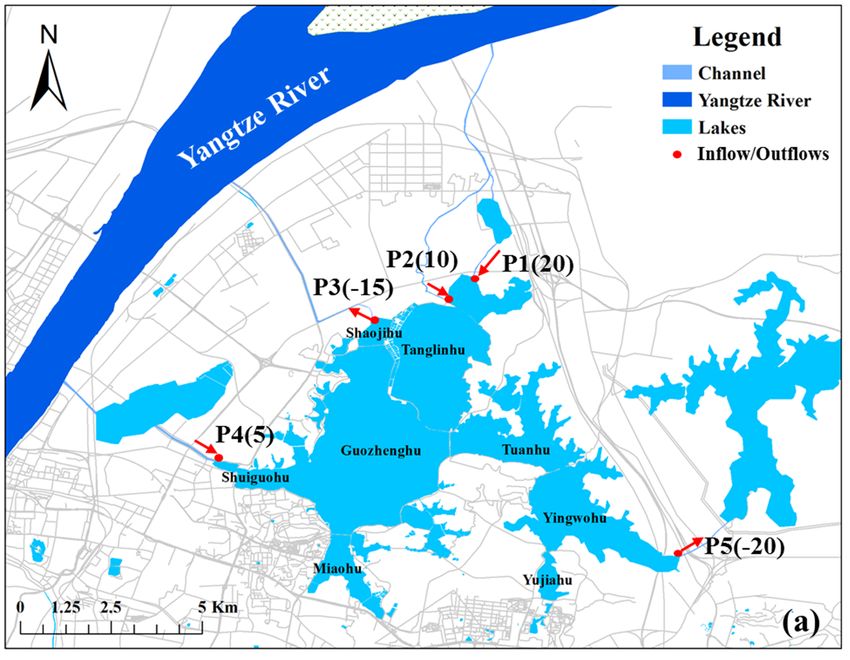
ISPRS Int. J. Geo-Inf. 2019, 8, 18                                                                                10 of 22

water quality standard [27] and presented in Figure 6b. It can be seen that water qualities in most bays
are worse than Class III. According to the target of water quality improvement, the water quality in
Lake Donghu must meet the Class III standard.
     In addition to Lake Donghu, the other urban lakes shown in Figure 6a also have serious
eutrophication problems. To improve the water quality of the lake groups, the Wuhan Municipal
Government lunched a water diversion project. The project was intended to dilute and flush the
nutrient concentrations from the lakes and decrease the residence time (or self-purification rates) by
diverting water from the Yangtze River. Water diversion has been proven to be a successful strategy
for improving water quality; it has been implemented in many Chinese lakes such as Taihu [28],
Chaohu [29], and Dianchi [30]. Previous water diversion projects suggest that it is necessary and helpful
to simulate hydrodynamic and water quality processes under different water diversion scenarios.
This section illustrates how to use the LMS to setup a FVCOM-LAKE model for Lake Donghu. Then,
the model was used to study the effects of water diversion on the change in hydrodynamics and
improvement of the water quality under different water diversion scenarios.

3.2. Model Setup
      To generate the computational grid, the bathymetry and lake boundary were collected.
The bathymetry was obtained from a filed investigation conducted in 2006. The grid was generated
using the LMS; it comprises 3476 nodes and 6067 triangular elements with approximate minimum and
maximum element sides of 40 and 60 m, respectively. The maximum water depth was approximately
4.5 m, and the minimum depth was artificially set at 0.5 m at the lakeshore. Nodes were not allowed
to be wet and dry. Depth levels were specified as sigma coordinates (terrain following) where the
depth levels are equally spaced in the water column. The model has four sigma coordinate levels; each
layer is 25% of the total water column depth. The bottom roughness was set to 0.0025 according to
similar lakes.
      The model simulation period ranged from 1 May 2011 to 31 July 2011. Data used to set the diving
forces, boundary and initial conditions during the period were collected from different sources. Hourly
meteorological data were obtained from a meteorological station near Lake Donghu. The original
format of the meteorological data was an Excel file. LMS was used to transform the original data into a
format acceptable by FVCOM-LAKE.
      The initial water level and water temperature was set to 19.15 m and an isothermal temperature
of 15 ◦ C everywhere according to the observed values on March 1, 2011. The initial flow velocity was
set at 0 m s−1 . The initial values for the water quality state variables were specified separately for each
bay based on observations (see Table 1). Investigations of pollution sources, including point sources
and nonpoint sources in the lake area, were conducted in 2011. The nonpoint sources were generalized
as point sources in the simulation. In total, seven major point-loadings entering the lake were specified.
Based on the Courant–Friedrichs–Lewy (CFL) criterion, the internal mode time step of the integration
was 300 s, while the external mode time step was 15 s.

                   Table 1. Initial values of the water quality variables in the bays of Lake Donghu.

                           DO          NH4         NO3         ON          PO4         OP         CBOD         CHL
           Bay
                         (mg L−1 )   (mg L−1 )   (mg L−1 )   (mg L−1 )   (mg L−1 )   (mg L−1 )   (mg L−1 )   (µg L−1 )
     Guozhenghu              8.35      0.031       0.026       0.103       0.024       0.008       4.21       20.17
      Tanglinhu              8.50      0.039       0.056       0.115       0.030       0.010       1.79        12.5
      Yingwohu               8.67      0.066       0.022       0.332       0.017       0.009       1.42       21.6
       Tuanhu                8.45      0.199       0.066       0.115       0.021       0.007       1.78        19.8
       Miaohu                7.98      2.560       0.853       2.787       0.360       0.124       9.13        95.6
      Shuiguohu              4.62      0.159       0.053       0.298       0.117       0.043       6.66       28.89
       Shaojihu              8.70      0.129       0.043       0.129       0.054       0.018       4.95        22.5
       Yujiahu               8.73      0.118       0.039       0.342       0.084       0.036       5.56        25.2
ISPRS Int. J. Geo-Inf. 2019, 8, 18 11 of 22
3.3. Model Calibration
Continuous observations of the water levels and water flow speed were unavailable for Lake
Donghu, so alternatively daily averaged water temperatures measured at station T1 were used to
calibrate the hydrodynamic model parameters. Monthly water quality observations made at stations
W1-W5 were used to calibrate WASP model parameters.
The calibration was manually accomplished in a trial-and-error manner. For the hydrodynamic
model, parameters related to the Mellor and Yamada turbulence model were set at the same values as
the ones used in other hydrodynamic models. Similarly, the non-dimensionless viscosity parameter in
the Smagorinsky formula was set to a constant value of 0.2. For the water quality model, the initial
values of the parameters (Table 2) used in the WASP were specified based on published field studies
performed on similar lakes and literature reviews, and previous WASP applications. Then, some of the
key parameters were further tuned.
Table 2. Parameter values used in the WASP water quality model.
Symbol Definition Value Unit
Kdeox Deoxygenation rate at 20 degree 0.1 c day−1
knitr Nitrification rate 0.35 c day−1
Kresp Phytoplankton respiration rate 0.1 d day−1
Kdeni Denitrification rate 0.08 c day−1
Kgrow Optimum phytoplankton growth rate 1.0 c day−1
Kmort Natural mortality rate of phytoplankton 0.1 c day−1
Kmine1 Organic nitrogen mineralization rate 0.075 c day−1
Kmine2 Organic phosphorus mineralization rate 0.2 c day−1
KCBOD Half-saturation constant for DO limitation of CBOD oxidation 0.5 c mg O2 L−1
Knitr Half-saturation constant for DO limitation of nitrification 0.5 e mg O2 L−1
Kdnf Half-saturation constant for DO limitation of denitrification 0.1 c mg O2 L−1
KNO3 Half-saturation constant for uptake of nitrate uptake 0.014 b mg N L−1
KPO4 Half-saturation constant for phosphorus uptake 0.003 b mg P L−1
Tempreae Temperature coefficient for reaeration 1.028 c Unitless
Tempnitr Temperature coefficient of nitrification 1.08 c Unitless
Tempresp Temperature coefficient of phytoplankton respiration 1.08 c Unitless
Tempdeni Temperature coefficient of denitrification 1.08 c Unitless
Tempgrow Temperature coefficient of optimum growth 1.066 c Unitless
Tempmort Temperature coefficient of phytoplankton mortality 1.08 c Unitless
Tempmine1 Temperature coefficient of nitrogen mineralization 1.08 c Unitless
Tempmine2 Temperature coefficient for organic phosphorus mineralization 1.08 c Unitless
Tempsod Temperature coefficient of sediment oxygen demand (SOD) 1.08 c Unitless
vPHY Phytoplankton settling velocity 0.5 a m day−1
vON Settling velocity of particulate organic nitrogen 0.5 a m day−1
vOP Settling velocity of particulate organic phosphorus 0.5 a m day−1
vCBOD Settling velocity of CBOD 0.5 c m day−1
SOD Sediment oxygen demand 0.3 c g O2 m−2 day−1
a This study, b Dortch [31], c Ambrose, et al. [23], d Geider [32], e Stenstrom & Poduska [33].
3.4. Scenario Design
To investigate the influence of diversion from the Yangtze River to Lake Donghu, three diversion
scenarios were designed (Table 3):
(1) The first scenario, named S1 (Figure 7a), has three inlets, P1, P2, and P3, and two outlets, P4 and
P5. P1 and P2 divert water from the Yangtze river into Tanglin bay with inflows of 20 m3 s−1 and
10 m3 s−1 , respectively; P3 diverts water from Lake Shahu into Shuiguo bay with an inflow of
5 m3 s−1 ; P4 drains water from Yingwo bay to Lake Yanxihu with an outflow of 20 m3 s−1 ; and
P5 drains water from Guozheng bay to the Yangtze River with an outflow of 20 m3 s−1 ;
(2) The second scenario, named S2 (Figure 7b), has two inlets, P1 and P2, with inflows of 25 m3 s−1
and 10 m3 s−1 , respectively, and three outlets, P3, P4 and P5, with outflows of 5 m3 s−1 , 20 m3 s−1 ,
and 10 m3 s−1 , respectively;ISPRS Int. J. Geo-Inf. 2019, 8, x FOR PEER REVIEW 12 of 22
(2) The second scenario, named S2 (Figure 7b), has two inlets, P1 and P2, with inflows of 25 m3 s−1
ISPRS and
Int. J.10
Geo-Inf.
m3 s2019, 8, 18and three outlets, P3, P4 and P5, with outflows of 5 m3 s−1, 20 12
−1, respectively, m3ofs22
−1,
and 10 m3 s−1, respectively;
(3) The third scenario, named S3 (Figure 7c), only has one inlet, P3, with an inflow of 35 m3 s−1, and
(3) The third scenario, named S3 (Figure 7c), only has one inlet, P3, with an inflow of 35 m3 s−1 ,
four outlets, P1, P2, P4 and P5, with outflows of 5 m3 s−1, 35 m 3 s−1, 20 m3 s−1, and 5 m3 s−1,
and four outlets, P1, P2, P4 and P5, with outflows of 5 m s−1 , 5 m3 s−1 , 20 m3 s−1 , and
respectively.
5 m3 s−1 , respectively.
The calibrated model was run to simulate each scenario for July 2011. All scenarios used the
The calibrated model was run to simulate each scenario for July 2011. All scenarios used the
same driven forces and point loadings but different inflow/outflow boundary conditions. To make a
same driven forces and point loadings but different inflow/outflow boundary conditions. To make
comparison between scenarios, a set of indicators was designed (Table 4). These indicators could be
a comparison between scenarios, a set of indicators was designed (Table 4). These indicators could
grouped into two categories. The first category contains indicators that describe hydrodynamic
be grouped into two categories. The first category contains indicators that describe hydrodynamic
characteristics, while the indicators in the second category describe improvements of water quality.
characteristics, while the indicators in the second category describe improvements of water quality.
Table 3. Water diversion scenarios.
Table 3. Water diversion scenarios.
Scenario ID Inlet & Inflow Discharge Outlet & Outflow Discharge
Scenario ID Inlet & Inflow Discharge Outlet & Outflow Discharge
P1: 20 m3 s−1
3 s−1 P4: −20 m3 s−1
S1 P2:P1:1020mm3 s−1
3 s−1 P4: −20 m3 s−1 3 −1
S1 P2: 10 m P5: −15 m s
P3: 5 m 3 s−1 P5: −15 m3 s−1
P3: 5 m s−1
3
P3: −5 m3 s−1
P1: 25 m3 3s−1−1 P3: −5 m3 s−1
S2 P1: 25 m s
S2 P2: 1010mm
33s−1s−1 P4: −P4: −20
20 m m1 3 s−1
3 s−
P2: −
P5: −P5: −10s m1 3 s−1
10 m3
P1: −P1:
5 m−5 m1 s
3 s− 3 −1
P2: −P2: 3 −
5 m−5s m1 3 s−1
S3 S3 P3:
P3: 33
3535mm s−1s−1 3 s−1 3 −1
P4: −P4:
20 m−20 m s
P5: −P5:
5 m−53 s−1
m3 s−1
Note: the outflow discharge is represented by negative value.
Note: the outflow discharge is represented by negative value.
Figure 7. Cont.ISPRS Int. J. Geo-Inf. 2019, 8, 18 13 of 22
ISPRS Int. J. Geo-Inf. 2019, 8, x FOR PEER REVIEW 13 of 22
Figure 7. Water
Waterdiversion
diversionscenario
scenariodesign:
design:(a)(a)
scenario S1, S1,
scenario (b) (b)
scenario S2, and
scenario (c) scenario
S2, and S3. The
(c) scenario S3.
values in brackets indicate discharge of inflow/outflow. The unit of the discharge is cubic meters
The values in brackets indicate discharge of inflow/outflow. The unit of the discharge is cubic meters per
second.
per Positive
second. values
Positive indicate
values inflows
indicate andand
inflows negative values
negative indicate
values outflows.
indicate outflows.ISPRS Int. J. Geo-Inf. 2019, 8, 18 14 of 22
ISPRS Int. J. Geo-Inf. 2019, 8, x FOR PEER REVIEW 14 of 22
Table
Table4.4.Indicators.
Indicators.
CategoryCategory Indicator
Indicator Unit Unit
Average velocity cm s−1
Average velocity cm s−1
Hydrodynamics
Hydrodynamics Velocity range
Velocity range cm s−1 cm s−1
Proportion of stagnant water
Proportion of stagnant water area area % %
Change
Change in TN
in TN concentration
concentration % %
Water Quality
Water Quality
Change
Change in concentration
in TP TP concentration % %
4.4.Results
Resultsand
andDiscussions
Discussions
4.1.
4.1.Calibration
CalibrationResults
Results
Figure
Figure88shows
showsaacomparison
comparisonofofsimulated
simulatedand andobserved
observeddaily
dailywater
watertemperature
temperatureatatlocation
locationT1.
T1.
The
Thevalue
valueof 2 2
ofRR indicates
indicatesthat
thatthe
themodel
modeladequately
adequatelysimulated
simulatedaavariation
variationininthe
thewater
watertemperature.
temperature.
The
Theresults
resultsofofthethesimulated
simulatedcurrents
currentsare
arevisualized
visualizedusing
usingthethe
visualization
visualizationtool of LMS
tool (Figure
of LMS 9). It
(Figure 9).
can be be
It can seen
seenthat
thatthethe
model
modelreproduced
reproduced the main
the mainfeatures
featuresofofthe
thewind-driven
wind-drivencirculation
circulationininthe
thelake
lake
quite
quitewell.
well. The
The model
model calibration
calibration results of TN
TN and
and TP
TPfor
forStations
StationsW1,
W1,W2,
W2,W3,W3,andandW4W4areareshown
shown in
in Figures
Figures 10 10
andand 11, 11, respectively.
respectively. In general,
In general, the model
the model provided
provided a reasonable
a reasonable reproduction
reproduction of
of patterns
patterns and acceptable
and acceptable magnitudes
magnitudes for waterfor waterconstituents.
quality quality constituents.
Comparisonofofsurface
Figure8.8.Comparison
Figure surfacewater
watertemperature
temperatureatatSite
SiteT1.
T1.ISPRS Int. J. Geo-Inf. 2019, 8, 18 15 of 22
ISPRS
ISPRS Int.
Int. J.J. Geo-Inf.
Geo-Inf. 2019,
2019, 8,
8, xx FOR
FOR PEER
PEER REVIEW
REVIEW 15
15 of
of 22
22
Figure 9.
9. Simulated
Figure 9.
Figure Simulated depth-averaged
Simulated circulation
depth-averaged circulation
depth-averaged on
on 555July
circulation on July 2011.
July2011.
2011.
Figure 10.Comparison
Figure 10.
10. Comparisonof
Comparison ofsimulated
of simulatedand
simulated observed
and
and TNTN
observed
observed at at
TN four bays:
at four
four (a) (a)
bays:
bays: Tanglin Bay;Bay;
(a) Tanglin
Tanglin (b) Guozheng
Bay; (b) Bay;
(b) Guozheng
Guozheng
(c)
Bay;Shuiguo
Bay; (c) Bay;
(c) Shuiguo and
Shuiguo Bay;(d) Yingwo
Bay; and
and (d) Bay.
(d) Yingwo
Yingwo Bay.
Bay.ISPRS Int. J. Geo-Inf. 2019, 8, 18 16 of 22
ISPRS Int. J. Geo-Inf. 2019, 8, x FOR PEER REVIEW 16 of 22
Figure 11. Comparison of simulated and observed TP at four bays: (a) Tanglin Bay; (b) Guozheng Bay;
Figure 11. Comparison of simulated and observed TP at four bays: (a) Tanglin Bay; (b) Guozheng Bay;
(c) Shuiguo Bay; and (d) Yingwo Bay.
(c) Shuiguo Bay; and (d) Yingwo Bay.
4.2. Scenario Analysis
4.2. Scenario Analysis
4.2.1. Change of Lake Circulation Pattern
4.2.1. Change of Lake Circulation Pattern
After implementing the water diversion project, hydrodynamic characteristics and circulation
After
patterns would implementing the water
be dramatically diversion
changed. project,
Figure hydrodynamic
12 compares characteristics
the circulation andofcirculation
patterns the three
patterns
scenarioswould on the be lastdramatically changed.period.
day of the simulation Figure For12 compares
scenario S1the circulation
(Figure patterns
12a), the movementof the three
of water
scenarios
develops in onthe theentire
last day
lake of the
area simulation
under period.effects
the combined For scenario
of waterS1 (Figureat12a),
diversion two the movement
inlets (P1, P2) andof
water develops in the entire lake area under the combined effects
drainage at three outlets (P3, P4 and P5). The water diverted into the lake from P1 and P2 is moved of water diversion at two inlets
(P1, P2) andand
southward drainage at three into
then divided outlets
two(P3, P4 and one
branches: P5). branch
The water diverted
is turned into the
around andlake frominto
merges P1 and
the
P2 is moved
water diverted southward
from P4,and andthen
then,divided
the mergedinto two branches:
water continues oneto branch
be movedis turned aroundand
northward anddrained
merges
into
out of thethewater
lakediverted
from P3;from P4, and
the other then, is
branch the merged
moved water continues
eastward and finally to discharges
be moved northward and
at P5. Overall,
drained
water inout the of the lake
larges baysfrom(e.g.,P3; the otherTanglin,
Guozheng, branch is movedand
Yingwo, eastward
Shuiguo andBays)
finally discharges
moves faster, at P5.
while
Overall, water in the larges bays (e.g., Guozheng, Tanglin, Yingwo, and
the water movement in the small lake branches is slow. It can also be seen that a local circulation is Shuiguo Bays) moves faster,
while
developed the water
in themovement
south partinofthe thesmall lake branches
Guozheng bay, underis slow. It can also
the driving be of
effect seen
thethat a local circulation
circulation, the water
is
in developed
Miao Bay flows in thenorthward.
south partThis of the Guozheng
circulation bay, under
is beneficial to the drivingthe
improving effect of the
water circulation,
quality the
of the Miao
water in Miao Bay flows northward. This circulation is beneficial to
Bay but also inevitably brings high-concentration pollutants in the Miao Bay into the main lake area. improving the water quality of
the MiaoIn theBay but also
second inevitably
scenario brings12b),
S2 (Figure high-concentration
the freshwater ispollutants
diverted fromin theP1 Miao
andBay into the
P2 flows main
through
lake
Tanglinarea.Bay before being divided into two branches near the road: one branch is moved southeastward
In the second
and finally dischargedscenario S2 the
at P5; (Figure
other12b),branchthe freshwater
is turned aroundis diverted
and from P1 and P2
then further flows into
divided through
two
Tanglin
subbranches, Bay before
in which being divided into
one subbranch two branches
is moved northward near and thedischarged
road: oneat branch
P3, andisthemoved
other
southeastward
subbranch is moved and finally
in an Sdischarged
path and isatdischarged
P5; the otherat P4. branch
Comparingis turned around
scenarios S1and
andthen
S2, itfurther
can be
divided
determined into that
two thesubbranches,
circulationinpattern
which is one subbranch
totally differentis moved northward
in Guozheng Bay and
and discharged
Shuiguo Bay at but
P3,
and the other
is similar subbranch
in Tanglin Bayisandmoved in anBay.
Yingwo S path and is discharged
Compared with thatatinP4. Comparing
scenario scenarios
S1, the S1 and
water flow in
S2, it can be determined that the circulation pattern is totally different
Guozheng bay under scenario S2 moves forward in a roundabout way, and the flow velocity is greatly in Guozheng Bay and Shuiguo
Bay but isaffecting
affected, similar in Tanglin
the Bayof
efficiency and Yingwo
water Bay. Compared with that in scenario S1, the water flow
renewal.
in Guozheng
Under scenariobay under scenario
S3 (Figure 12c),S2the
moves forwardininShuiguo
flow velocity a roundabout way, and
Bay is greatly the flowbyvelocity
accelerated diverting is
greatly affected, affecting the efficiency of water renewal.
freshwater from P4, then the diverted water moves northward and is divided into three branches:
Under scenario S3 (Figure 12c), the flow velocity in Shuiguo Bay is greatly accelerated by
diverting freshwater from P4, then the diverted water moves northward and is divided into three
branches: the first branch continues to move northward and is discharged at P3; the second branchISPRS Int. J. Geo-Inf. 2019, 8, 18 17 of 22
the first branch continues to move northward and is discharged at P3; the second branch also
ISPRS Int. J. Geo-Inf. 2019, 8, x FOR PEER REVIEW
moves
17 of 22
northward and is discharged at P1 and P2; and the third branch moves eastward and is discharged
at P5.also moves northward and is discharged at P1 and P2; and the third branch moves eastward and is
discharged
Table at P5.
5 compares the hydrodynamic indicators under the three water diversion scenarios.
Table 5 compares
Under scenarios S1, S2, and theS3,
hydrodynamic indicators
average velocities areunder theand
1.9,1.5 three1.3water −1 , respectively,
cm sdiversion scenarios.and
Undervelocity
scenarios S1, S2, and S3, average
− 1 velocities are 1.9,1.5 and 1.3 cm s-1, respectively, and velocity ranges
ranges are 44, 22 and 25 cm s , respectively. It can be seen that scenario S1 is the best for accelerating
are 44, 22 and 25 cm s-1, respectively. It can be seen that scenario S1 is the best for accelerating water
water flow velocity. However, scenario S2 the best for reducing stagnant water area.
flow velocity. However, scenario S2 the best for reducing stagnant water area.
Figure 12. Cont.ISPRS Int. J. Geo-Inf. 2019, 8, 18 18 of 22
ISPRS Int. J. Geo-Inf. 2019, 8, x FOR PEER REVIEW 18 of 22
Figure 12. Depth-averaged circulation on July 15, 2011 under scenarios S1 (a), S2 (b), and S3 (c).
Figure 12. Depth-averaged circulation on July 15, 2011 under scenarios S1 (a), S2 (b), and S3 (c).
Table
Table 5. Hydrodynamicindicators
5. Hydrodynamic indicators under
underdifferent
differentwater
waterdiversion scenarios.
diversion scenarios.
Scenarios
Hydrodynamic Indicators Scenarios
Hydrodynamic Indicators S1 S2 S3
Average velocity (cm s−1) S1 1.9 S2 1.5 S31.3
Average velocity
Velocity (cmss−−11))
range(cm 1.9 44 1.5 22 1.325
Velocity
Proportion range (cm
of stagnant s−1 ) area (%)
water 44 2.6 22 2.3 252.8
Proportion of stagnant water area (%) 2.6 2.3 2.8
4.2.2. Improvement of Water Quality
4.2.2. Improvement of Waterthe
Figure 13 compares Quality
spatial distribution of TN and TP concentrations in Lake Donghu after
implementing
Figure 13 compareswater diversion for 31
the spatial days underof
distribution theTNthree
andscenarios. In comparison
TP concentrations with the
in Lake initial after
Donghu
conditions, the concentrations of TN and TP are significantly decreased in most of the bays under all
implementing water diversion for 31 days under the three scenarios. In comparison with the initial
three scenarios. However, the TN and TP concentrations in Miao bay are still high under all scenarios.
conditions, the concentrations of TN and TP are significantly decreased in most of the bays under all
Water quality improvements are characterized by four indicators as shown in Table 6. Under
threescenarios
scenarios.S1,However,
S2, and S3, the TN and TP concentrations
TN concentrations are reduced byin Miao43.2%,
35.8%, bay are
andstill high
17.3%, under all scenarios.
respectively, and
TP concentrations are reduced by 52.5%, 41.7% and 16.7%, respectively. Thus, it caninbeTable
Water quality improvements are characterized by four indicators as shown seen 6. Under
that
scenarios S1, S2, and S3, TN concentrations are reduced by 35.8%, 43.2%, and 17.3%,
scenario S1 is the best for reducing the TP concentration and that S2 is the best for reducing the TN respectively,
and TP concentrations
concentration for theare reduced
entire by 52.5%, to
lake. According 41.7% andof16.7%,
the goal respectively.
the water diversion, Thus, it can
the water be seen
quality in that
LakeS1
scenario Donghu
is themust
best reach Class III. the
for reducing Based
TPon the threshold values
concentration of TN
and that S2 and TPbest
is the specified in Class III,
for reducing the TN
the percentage of lake areas that failed to reach the goal was calculated and is
concentration for the entire lake. According to the goal of the water diversion, the water qualitypresented in Table 6. in
Overall, scenarios S1 and S2 have similar effects towards improving water
Lake Donghu must reach Class III. Based on the threshold values of TN and TP specified in Class III, quality, and they
outperform scenario S3 with respect to all indicators.
the percentage of lake areas that failed to reach the goal was calculated and is presented in Table 6.
Through a comprehensive consideration of hydrodynamic and water quality indicators, we can
Overall, scenarios S1 and S2 have similar effects towards improving water quality, and they outperform
conclude the following: scenario S1 is the best for improving hydrodynamic indicators and for
scenario S3 with
reducing respect to all indicators.
TP concentrations, and scenario S2 is the best for reducing TN concentrations. Considering
that TP is the major controllingconsideration
Through a comprehensive of hydrodynamic
factor for improving andLake
water quality for water quality
Donghu, indicators,
scenario S1 is we
can conclude
thought tothe following:
be the scenario
best solution S1 isthe
to achieve thewater
best diversion
for improving
goal. hydrodynamic indicators and for
reducing TP concentrations, and scenario S2 is the best for reducing TN concentrations. Considering
that TP is the major controlling factor for improving water quality for Lake Donghu, scenario S1 is
thought to be the best solution to achieve the water diversion goal.You can also read