An inter-comparison of the mass budget of the Arctic sea ice in CMIP6 models
←
→
Page content transcription
If your browser does not render page correctly, please read the page content below

The Cryosphere, 15, 951–982, 2021
https://doi.org/10.5194/tc-15-951-2021
© Author(s) 2021. This work is distributed under
the Creative Commons Attribution 4.0 License.

An inter-comparison of the mass budget of
the Arctic sea ice in CMIP6 models
Ann Keen1 , Ed Blockley1 , David A. Bailey2 , Jens Boldingh Debernard3 , Mitchell Bushuk4 , Steve Delhaye5 ,
David Docquier6 , Daniel Feltham7 , François Massonnet5 , Siobhan O’Farrell8 , Leandro Ponsoni5 , José M. Rodriguez9 ,
David Schroeder7 , Neil Swart10 , Takahiro Toyoda11 , Hiroyuki Tsujino11 , Martin Vancoppenolle12 , and Klaus Wyser6
1 Met Office Hadley Centre, Exeter, UK
2 National Center for Atmospheric Research (NCAR), Boulder, CO, USA
3 Norwegian Meteorological Institute, Oslo, Norway
4 Geophysical Fluid Dynamics Laboratory (GFDL), Princeton, NJ, USA
5 Georges Lemaître Centre for Earth and Climate Research (TECLIM), Earth and Life Institute,

Université catholique de Louvain, Louvain-la-Neuve, Belgium
6 Rossby Centre, Swedish Meteorological and Hydrological Institute (SMHI), Norrköping, Sweden
7 Centre for Polar Observations and Modelling (CPOM), University of Reading, Reading, UK
8 CSIRO Oceans and Atmosphere, Aspendale, Victoria, Australia
9 Agencia Estatal de Meteorología (AEMET), Madrid, Spain
10 Environment and Climate Change Canada (ECCC), Canadian Centre for Climate Modelling and Analysis,

Victoria, BC, Canada
11 Meteorological Research Institute, Japan Meteorological Agency, Tsukuba, Japan
12 Laboratoire d’Océanographie et du Climat and Institut Pierre-Simon Laplace (LOCEAN-IPSL), Paris, France

Correspondence: Ann Keen (ann.keen@metoffice.gov.uk)

Received: 20 December 2019 – Discussion started: 19 February 2020
Revised: 14 December 2020 – Accepted: 16 December 2020 – Published: 24 February 2021

Abstract. We compare the mass budget of the Arctic sea            ferences between the models, and we have found a number
ice for 15 models submitted to the latest Coupled Model           of relationships between model formulation and components
Intercomparison Project (CMIP6), using new diagnostics            of the ice budget that hold for all or most of the CMIP6 mod-
that have not been available for previous model inter-            els considered here. The relative amounts of frazil and basal
comparisons. These diagnostics allow us to look beyond the        ice formation vary between the models, and the amount of
standard metrics of ice cover and thickness to compare the        frazil ice formation is strongly dependent on the value cho-
processes of sea ice growth and loss in climate models in a       sen for the minimum frazil ice thickness. There are also dif-
more detailed way than has previously been possible.              ferences in the relative amounts of top and basal melting,
   For the 1960–1989 multi-model mean, the dominant pro-          potentially dependent on how much shortwave radiation can
cesses causing annual ice growth are basal growth and frazil      penetrate through the sea ice into the ocean. For models with
ice formation, which both occur during the winter. The main       prognostic melt ponds, the choice of scheme may affect the
processes by which ice is lost are basal melting, top melting     amount of basal growth, basal melt and top melt, and the
and advection of ice out of the Arctic. The first two processes   choice of thermodynamic scheme is important in determin-
occur in summer, while the latter process is present all year.    ing the amount of basal growth and top melt.
The sea ice budgets for individual models are strikingly simi-       As the ice cover and mass decline during the 21st cen-
lar overall in terms of the major processes causing ice growth    tury, we see a shift in the timing of the top and basal melting
and loss and in terms of the time of year during which each       in the multi-model mean, with more melt occurring earlier
process is important. However, there are also some key dif-       in the year and less melt later in the summer. The amount

Published by Copernicus Publications on behalf of the European Geosciences Union.
952                         A. Keen et al.: An inter-comparison of the mass budget of the Arctic sea ice in CMIP6 models

of basal growth reduces in the autumn, but it increases in            For previous model inter-comparisons (CMIP3 and
the winter due to thinner sea ice over the course of the 21st      CMIP5), primarily only changes in ice extent, volume (or
century. Overall, extra ice loss in May–June and reduced ice       mass) and ice motion (Tandon et al., 2018; Rampal et al.,
growth in October–November are partially offset by reduced         2011) have been considered, as these quantities are readily
ice melt in August and increased ice growth in January–            available as model output that can be compared directly to
February. For the individual models, changes in the budget         one another and to observational or reanalysis references.
components vary considerably in terms of magnitude and             However, there is an emerging consensus that in order to
timing of change. However, when the evolving budget terms          understand the reasons for differences in projections of the
are considered as a function of the changing ice state itself,     ice state, we need to be able to look “behind the scenes” to
behaviours common to all the models emerge, suggesting             understand the balance of different processes that drive the
that the sea ice components of the models are fundamentally        evolving ice state and how these change as the ice declines.
responding in a broadly consistent way to the warming cli-            For the CMIP3 models, Holland et al. (2010) calculated
mate.                                                              the changes in ice mass due to melt, growth and divergence
   It is possible that this similarity in the model budgets may    using monthly mean model values of ice thickness and ve-
represent a lack of diversity in the model physics of the          locity. They found an appreciable variation in the size and
CMIP6 models considered here. The development of new               relative importance of changes in these budget components
observational datasets for validating the budget terms would       between the models as the sea ice declines. For individual
help to clarify this.                                              models, diagnostics may be available that allow a more com-
                                                                   prehensive decomposition of the model budget. For exam-
                                                                   ple, Keen and Blockley (2018) studied changes in the volume
                                                                   budget of the Arctic sea ice in a CMIP5 model under a range
1   Introduction                                                   of forcing scenarios, considering both annual and seasonal
                                                                   changes in the individual processes causing ice growth and
Sea ice is a key component of the climate system, and the          loss.
observed decline in Arctic ice cover provides a very visible          For the latest generation of sea ice models (the CMIP6
indicator of climate change. Between 1979 and 2018, Arctic         models), a Sea-Ice Model Intercomparison Project (SIMIP)
September sea ice extent has declined at a rate of nearly 13 %     has been established, which has defined a comprehensive set
per decade (IPCC, 2019). The ice has also thinned, and there       of diagnostics allowing for the intercomparison of the mass,
has been a transition to a greater coverage of younger ice: the    energy and freshwater budgets of the sea ice (Notz et al.,
proportion of Arctic ice cover that is more than 5 years old       2016). In this study we use these new diagnostics to present
decreased by 90 % between 1979 and 2018 (Kwok, 2018;               a first intercomparison of the mass budget of the sea ice for
Stroeve and Notz, 2018; IPCC, 2019). The ice also moves            15 of the CMIP6 models. Note that this is a subset of the
more quickly (Olason and Notz, 2014).                              CMIP6 models, just including those for which the required
   Global coupled climate models are the most comprehen-           outputs were available. We first look at the mean mass bud-
sive tools that we have for predicting how the Arctic ice will     get for a reference period to determine the similarities and
change in the future, as they can represent a range of pro-        differences between the model budgets during a period with
cesses that control the seasonal cycle of ice growth and melt,     relatively little change in the ice state. We then consider how
and so they have the potential to represent the changing na-       the budgets change as the ice declines during the 21st century
ture of the ice itself. However, model projections show a wide     and how changes in the budget components relate to changes
spread in the rate of ice decline, both during the period for      in the ice state and the global temperature.
which we have observations and also into the future as we             In Sect. 2 we describe the models and forcing scenarios
move towards a seasonally ice-free Arctic (Massonnet et al.        used, and in Sect. 3 we intercompare the modelled ice area
2012; Notz and Stroeve, 2016; SIMIP community, 2020).              and mass. In Sects. 4 and 5 we consider the mean mass bud-
   Some of this spread is an inevitable consequence of the in-     get during a reference period, and in Sect. 6 we investigate
ternal variability of the climate system, and the uncertainty      how the budget evolves during the 21st century. In Sect. 7 we
in future forcing. For example, Jahn et al. (2016) find that       summarize and discuss our results.
internal variability causes an uncertainty of 21 years in pre-
dicting the year in which the Arctic first becomes seasonally
ice-free using a large (40-member) ensemble of model runs,         2   Models and methodology
with an additional uncertainty of 5 years due to scenario un-
certainty. A similar degree of spread also occurs due to differ-   In this study we analyse data from 15 CMIP6 models, origi-
ences between the models’ representation of the sea ice and        nating from nine different modelling centres. We also analyse
other components of the climate system (Topál et al., 2020).       data from three configurations of the NEMO-CICE ocean–
Spread may also arise from differences in initial conditions       sea ice model forced by atmospheric reanalysis, which has a
(Hawkins and Sutton, 2009; Melia et al., 2015).                    similar formulation to one of the CMIP6 models used in this

The Cryosphere, 15, 951–982, 2021                                                      https://doi.org/10.5194/tc-15-951-2021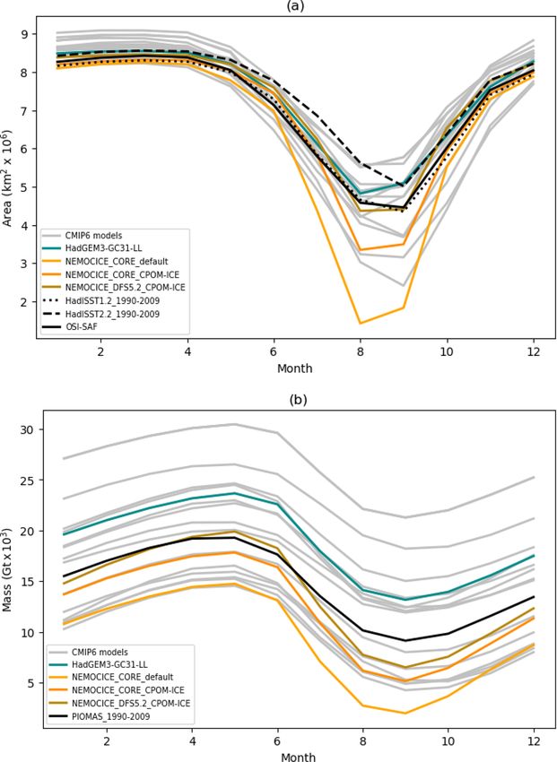
A. Keen et al.: An inter-comparison of the mass budget of the Arctic sea ice in CMIP6 models                                              953

Table 1. List of models and modelling centres participating in this study. Where two modelling centres are shown, the first analysed the
model outputs, and the second performed the model integrations.

                                                              No. of integrations
  Model name                           Modelling centre       Hist      SSP58.5     Notes
  HadGEM3-GC31-LL                      Met Office               4              4
  HadGEM3-GC31-MM                      Met Office               4              4
  UKESM1-0-LL                          Met Office              12              5
  EC-Earth3                            UCLouvain/AEMET          1              1    No explicit lateral melt
  EC-Earth3-Veg                        UCLouvain/SMHI           1              1    No explicit lateral melt, dynamics term missing
  MRI-ESM2                             MRI                      5              1    No explicit lateral melt or frazil ice formation
  CESM2-CAM                            NCAR                    11              2
  CESM2-WACCM                          NCAR                     3              2
  GFDL-CM4                             GFDL                     1              1    No explicit lateral melt
  GFDL-ESM4                            GFDL                     1              1    No explicit lateral melt
  CSIRO_ARCCSS_ACCESS-CM2              CSIRO                    1              1
  NorESM2-LM                           Met Norway               3              1
  NorESM2-MM                           Met Norway               1              1
  CanESM5                              ECCC                     3              3    Missing terms: frazil, lateral melt, evapsubl, dynamics
  IPSL_CM6A-LR                         IPSL                    32              6    No explicit lateral melt
  NEMOCICE_CORE_default                CPOM                     1                   Forced ocean–ice model (so no scenario data)
  NEMOCICE_CORE_CPOM-CICE              CPOM                     1
  NEMOCICE_DFS5.2_CPOM-CICE            CPOM                     1

study (HadGEM3-GC3.1-LL). These models, and the data                      – snow ice, ice formation due to the transformation of
provided from each, are listed in Table 1. Key details about                snow to sea ice due to surface flooding;
the formulation of each model are summarized in Table 2,
                                                                          – evapsubl, the change in ice mass due to evaporation and
with a brief description of each in Appendix A. For each
                                                                            sublimation;
model, the ice area and mass and the area-weighted monthly-
mean ice mass budget terms were calculated over the domain                – advection, the change in ice mass due to ice being ad-
shown in Fig. 1a, covering the Arctic Ocean basin (central                  vected into or out of the analysis domain.
Arctic plus the Beaufort, Chukchi, East Siberian, Laptev and
                                                                       The monthly mean data were calculated for the period 1960–
Kara seas) and the Barents Sea. Unless otherwise stated, all
                                                                       2100 from model integrations using the CMIP6 Hist forcing
results shown in the paper are integrals over this analysis re-
                                                                       scenario for the period 1960–2014 and SSP5-8.5 thereafter
gion and so do not represent the entire Northern Hemisphere
                                                                       (Gidden et al., 2019). The SSP5-8.5 scenario was primarily
ice-covered region, especially in winter. This will have an im-
                                                                       chosen because for the majority of participating modelling
pact on some of the values calculated. Most notably it may
                                                                       centres this was the first scenario to be run, but it also has the
affect the month of the seasonal maxima and minima for
                                                                       advantage of being the scenario with the highest warming
some quantities, but as values for the models and observa-
                                                                       signal. This means that we see relatively large changes in the
tional datasets are calculated over the same region, this is un-
                                                                       ice state and the budget terms during the 21st century, and
likely to affect the general conclusions. Multi-model means
                                                                       differences between the model budget terms are likely to be
are calculated by first averaging all the realizations for each
                                                                       more pronounced.
individual model (where appropriate) and then averaging the
                                                                          In order to better understand the relative roles of atmo-
resulting ensemble means. The mass budget terms are de-
                                                                       spheric forcing and sea ice model physics, results from three
fined in Appendix E of Notz et al. (2016) and summarized
                                                                       forced ocean–ice simulations are also included. All of them
here for completeness:
                                                                       use the same ocean and sea ice models as the UK CMIP6
  – basal growth, ice growth at the base of existing ice;              models (HadGEM3-GC31-LL, HadGEM3-GC31-MM and
                                                                       UKESM1-0-LL), with changes to both the parameter settings
  – frazil ice formation, ice formation in supercooled open            and the atmospheric forcing datasets. Further details of the
    water;                                                             settings and forcings used can be found in Table 3.
                                                                          We also compare the modelled ice state with a number of
  – top melt, melting at the top surface of the ice;                   observational and reanalysis datasets. We calculate the ice
  – basal melt, melting at the base of the ice;                        area over our analysis domain (Fig. 1) using monthly mean
                                                                       values for the years 1979 to 2015 from three observational
  – lateral melt, melting at the sides of the ice;                     products so that we take account of observational uncertainty.

https://doi.org/10.5194/tc-15-951-2021                                                            The Cryosphere, 15, 951–982, 2021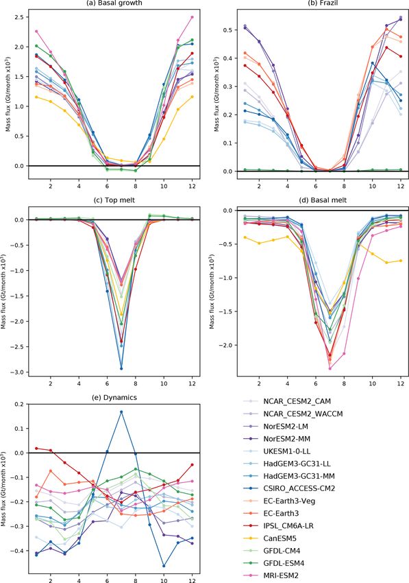
Table 2. Relevant information for all the CMIP6 models used in this study including a summary of the model subcomponents and resolution, along with details of several key physical
A. Keen et al.: An inter-comparison of the mass budget of the Arctic sea ice in CMIP6 models
https://doi.org/10.5194/tc-15-951-2021
aspects of the sea ice subcomponents. For thermodynamics, T13 denotes the mushy-layer scheme of Turner et al. (2013), whilst BL99 and MK89 denote fixed salinity profile schemes
of Bitz and Lipscomb (1999) and Mellor and Kantha (1989), respectively. For prognostic melt ponds, F12 denotes the “topographic” scheme of Flocco et al. (2012), whilst H13 denotes
the “level ice” scheme of Hunke et al. (2013). For rheology, EVP is the elastic–viscous–plastic scheme of Hunke and Dukowicz (1997).
Components, configurations, resolution UKESM1-0-LL HadGEM3-GC31-LL HadGEM3-GC31-MM AEMET_EC- SMHI_EC-Earth3- ACCESS-CM2 MRI-ESM2
Earth3 Veg
Sea ice model component (configuration) CICE 5.1.2 CICE 5.1.2 CICE 5.1.2 LIM3 LIM3 CICE 5.1.2 MRI. COM4.4
(GSI8.1) (GSI8.1) (GSI8.1) (GSI8.1)
Sea ice model resolution 1◦ (ORCA1) 1◦ (ORCA1) 0.25◦ (ORCA025) 1◦ (ORCA1) 1◦ (ORCA1) 1◦ 1◦ (long) ×
0.3–0.5◦ (lat)
Ocean model component (configuration) NEMO3.6 (GO6) NEMO3.6 (GO6) NEMO3.6 (GO6) NEMO3.6 NEMO3.6 MOM5.1 MRI. COM4.4
(ACCESS-OM)
Ocean model resolution 1◦ (ORCA1) 1◦ (ORCA1) 0.25◦ (ORCA025) 1◦ (ORCA1) 1◦ (ORCA1) 1◦ 1◦ (long) ×
0.3–0.5◦ (lat)
Atmosphere model component (configuration) MetUM (GA7.1) MetUM (GA7.1) MetUM (GA7.1) IFS (cycle36r4) IFS (cycle36r4) MetUM (GA7.1) MRI-AGCM 3.5
Atmosphere model resolution 135 km (N96) 135 km (N96) 60 km (N216) 80 km (T255L91) 80 km (T255L91) 135 km (N96) 120 km (TL159)
Sea ice model specifics
Rheology EVP EVP EVP EVP EVP EVP EVP
Ice thickness distribution (ITD) Prognostic Prognostic Prognostic Prognostic Prognostic Prognostic Prognostic
No. of thickness categories Five Five Five Five Five Five Five
Radiation scheme Dual band (CCSM3) Dual band (CCSM3) Dual band (CCSM3) Broadband Broadband Dual band Dual band (CCSM3)
(CCSM3)
Penetration of SW into ocean No No No Yes Yes No Yes
Melt ponds Prognostic (F12) Prognostic (F12) Prognostic (F12) Prescribed albedo Prescribed albedo Prognostic (F12) Parameterized
reduction reduction
Thermodynamics BL99 BL99 BL99 BL99 + prognostic BL99 + prognostic BL99 MK89
salinity profile salinity profile
No. of ice (snow) layers Four (one) Four (one) Four (one) Two (one) Two (one) Four (one) One (zero)
Minimum lead fraction None None None 0.003 0.003 None None
Minimum frazil thickness 5 cm 5 cm 5 cm 10 cm 10 cm 5 cm –
Coupling, time-stepping
Sea ice model time step 30 min 30 min 20 min 45 min 45 min 30 min 30 min
Ice–ocean coupling frequency 30 min 30 min 20 min 45 min 45 min 30 min 30 min
Ice–atmosphere coupling frequency 20 min 20 min 20 min 45 min 45 min 20 min 60 min
(180 min) (180 min) (60 min) (180 min)
Components, configurations, resolution GFDL-CM4 GFDL-ESM4 CanESM5 CESM2-CAM CESM2- NorESM-LL NorESM-MM IPSL-CM6A-LR
WACCAM
Sea ice model component (configuration) SIS2 SIS2 LIM2 CICE 5.2.1 CICE 5.2.1 CICE 5.2.1 CICE 5.2.1 LIM3
Sea ice model resolution 0.25◦ 0.5◦ 1◦ (ORCA1) 1◦ (gx1) 1◦ (gx1) 1◦ (tn1v4) 1◦ (tn1v4) 1◦
Ocean model component (configuration) MOM 6 MOM 6 NEMO 3.4.1 POP 2.0.1 POP 2.0.1 BLOM BLOM NEMO 3.6
(OM4.0) (OM4.0)
Ocean model resolution 0.25◦ 0.5◦ 1◦ (ORCA1) 1◦ (gx1) 1◦ (gx1) 1◦ (tn1v4) 1◦ (tn1v4) 1◦
Atmosphere model component (configuration) GFDL-AM (AM4.0) GFDL-AM (AM4.0) CanAM CAM 6 CAM 6 NorCAM6 NorCAM6 LMDZ6
The Cryosphere, 15, 951–982, 2021
Atmosphere model resolution 100 km 100 km 2.8◦ (T63) 0.9◦ (long) × 0.9◦ (long) × 1.9◦ (long) × 0.9◦ (long) × 2.5◦ × 1.3◦ (144 × 142)
1.25◦ (lat) 1.25◦ (lat) 2.5◦ (lat) 1.25◦ (lat)
Sea ice model specifics
Rheology EVP EVP EVP EVP EVP EVP EVP EVP
Ice thickness distribution (ITD) Prognostic Prognostic Diagnostic Prognostic Prognostic Prognostic Prognostic Prognostic
No. of thickness categories Five Five One Five Five Five Five Five
Radiation scheme delta-Eddington delta-Eddington Multi-band delta-Eddington delta-Eddington delta-Eddington delta-Eddington broadband
Penetration of SW into ocean Yes Yes Yes Yes Yes Yes Yes Yes
Melt ponds Parameterized Parameterized Parameterized Prognostic (H13) Prognostic (H13) Prognostic (H13) Prognostic (H13) Prescribed albedo reduction
Thermodynamics BL99 BL99 Semtner zero layer T13 T13 T13 T13 BL99 + prognostic salinity profile
No. of ice (snow) layers Four (one) Four (one) – Eight (three) Eight (three) Eight (three) Eight (three) Two (one)
Minimum lead fraction None None 1.0e-6 None None None None 0.003
Minimum frazil thickness None None 5 cm 5 cm 5 cm 5 cm 5 cm 10 cm
Coupling, time-stepping
Sea ice model time step 20 min 20 min 60 min 30 min 30 min 30 min 30 min 90 min
Ice–ocean coupling frequency 60 min 60 min 60 min 30 min 30 min 30 min 30 min 90 min
954
Ice–atmosphere coupling frequency 20 min 20 min 180 min 60 min 60 min 30 min 30 min 90 min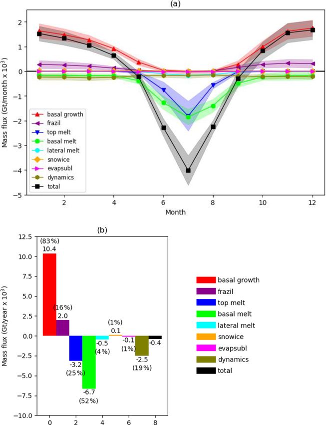
A. Keen et al.: An inter-comparison of the mass budget of the Arctic sea ice in CMIP6 models                                        955

Table 3. Relevant information describing the CPOM NEMO-CICE forced models used in this study. Including details of the atmospheric
forcing datasets used and the changes in the CICE sea ice physics used in the different simulations. Also included is the HadGEM3-GC3.1-
LL model for reference. All physics options not included in this table – including those shown in Table 2 above – are identical to the
HadGEM3-GC3.1-LL model. CORE II is the CORE2 surface forcing dataset of Large and Yeager (2009), whilst DFS5.2 is the Drakkar
forcing set of Dussin et al. (2016). For rheology, EVP is the elastic–viscous–plastic scheme of Hunke and Dukowicz (1997), and EAP is the
elastic–anisotropic–plastic scheme of Tsamados et al. (2013). The melt pond max fraction term (rfracmax) determines the maximum fraction
of meltwater added to the ponds within the Flocco et al. (2012) “topographic” prognostic melt pond scheme.

                              CPOM_NEMOCICE_            CPOM_NEMOCICE_             CPOM_NEMOCICE_            HadGEM3-GC3.1-LL
                              CORE_default              CORE_CPOM-CICE             DFS5.2_CPOM-CICE
   Atmospheric forcing
   Dataset                    CORE II                   CORE II                    DFS5.2                    MetUM coupled
   Resolution                 ∼ 200 km                  ∼ 200 km                   ∼ 80 km                   ∼ 135 km (N96)
   Frequency                  6 hourly                  6 hourly                   6 hourly                  3 hourly
   Sea ice model physics
   Rheology                   EVP                       EAP                        EAP                       EVP
   Sea ice conductivity       “default” (Maykut and     “bubbly brine” (Pringle    “bubbly brine” (Pringle   “default” (Maykut and
                              Untersteiner, 1971)       et al., 2007)              et al., 2007)             Untersteiner, 1971)
   Sea ice emissivity         0.95                      0.976                      0.976                     0.95
   Melt pond max fraction     85 %                      50 %                       50 %                      85 %
   (rfracmax)
   Blown snow scheme          None                      Schroder et al. (2019)     Schroder et al. (2019)    None

   We use the second version of the global sea ice concen-             3     Model inter-comparison of mean sea ice state
tration climate data record (OSI-450) from the European Or-
ganisation for the Exploitation of Meteorological Satellites           We first compare the ice area and mass simulated by the dif-
(EUMETSAT) Ocean Sea Ice Satellite Application Facil-                  ferent models. We consider the seasonal cycle for the period
ity (http://osisaf.met.no/p/ice/ice_conc_cdr_v2.html, last ac-         1990–2009, in order to compare model results to present-day
cess: 19 November 2019, OSI-SAF, 2017; Lavergne et al.,                observations and the PIOMAS reanalysis. We also consider
2019).                                                                 the evolution of the ice area and mass from 1960 to 2100, so
   We use the first and second versions of the Met Of-                 that we can put the budget changes into context. Note that the
fice Hadley Centre’s sea ice and sea surface temper-                   values of ice area and mass shown here, for both the models
ature dataset: HadISST1.2 (https://www.metoffice.gov.uk/               and observational datasets, are values for the Arctic domain
hadobs/hadisst/, last access: 22 January 2018, Rayner et               shown in Fig. 1a and do not represent the whole ice-covered
al., 2003) and HadISST.2.2 (https://www.metoffice.gov.uk/              region.
hadobs/hadisst2/, last access: 22 January 2018, Titchner and
Rayner, 2014).                                                         3.1    1990–2009 seasonal cycle
   For ice mass we use monthly mean sea ice thickness for the
years 1960 to 2019 from the Pan-Arctic Ice-Ocean Modeling              During the period 1990–2009, there is a spread of 0.7 mil-
and Assimilation System (PIOMAS) (http://psc.apl.uw.edu/               lion square kilometres in the March ice area simulated by
research/projects/arctic-sea-ice-volume-anomaly/data/ (last            the models (Fig. 1a). Despite the winter ice cover being
access: 22 January 2018), Zhang and Rothrock, 2003) to cal-            bounded to some extent by the analysis region, the mod-
culate the ice volume, which is then converted to mass using           elled values range from 8.4 to 9.1 million square kilometres,
the constant value of 917 kg m−3 for the ice density used in           compared with a range of 8.2 to 8.7 million square kilome-
PIOMAS. While this is not an observational dataset, it pro-            tres for the three observational datasets. The observational
vides a useful reference as it has been well studied and vali-         range as quoted here is the spread in the ±1 standard de-
dated against observations (for example Stroeve et al., 2014;          viation limits for the three datasets. In September we see a
Wang et al., 2016) and has a well-quantified measure of un-            much larger spread in modelled ice area (3.4 million square
certainty (Schweiger et al., 2011).                                    kilometres), although most models fall within the observa-
                                                                       tional range, which is larger for September than for March.
                                                                       One model in particular (NCAR_CESM2_CAM) has an es-
                                                                       pecially large seasonal cycle and low ice area in September,
                                                                       possibly because of its relatively low ice mass (Fig. 1b and

https://doi.org/10.5194/tc-15-951-2021                                                          The Cryosphere, 15, 951–982, 2021
956 A. Keen et al.: An inter-comparison of the mass budget of the Arctic sea ice in CMIP6 models
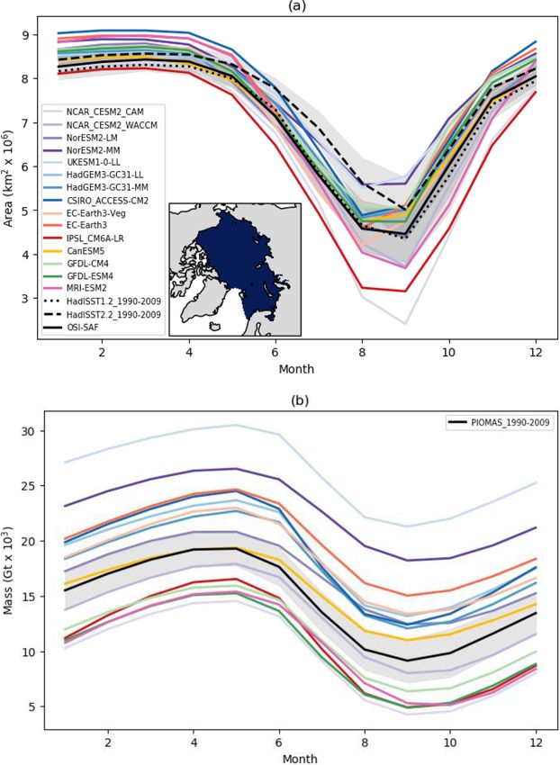
Figure 1. Seasonal cycles of (a) ice area and (b) ice mass for the reference period 1990–2009, for the CMIP6 models. Where more than
one model integration is available, the values are ensemble means. Also shown are data from the (a) HadISST1.2 (Rayner et al., 2003),
HadISST.2.2 (Titchner and Rayner, 2014) and OSI-SAF (OSI-SAF, 2017) observational datasets and (b) PIOMAS reanalysis (Zhang and
Rothrock, 2003) for the same period. The shaded regions show ±1 standard deviation in the monthly values. Data are summed over the
analysis domain shown in (a), which is defined using the NSIDC Arctic regional masks (https://nsidc.org/data/polar-stereo/tools_masks.
html#region_masks, last access: 31 January 2018), where we include the following regions: central Arctic Ocean, Beaufort Sea, Chukchi
Sea, East Siberian Sea, Laptev Sea, Kara Sea and Barents Sea.
discussed below). The magnitude of the modelled seasonal calculated over our analysis region) in August or have Au-
cycle in ice area varies between 3.2 and 6.0 million square gust and September values that are very similar.
kilometres. The observational datasets have their minimum There is a large spread in modelled values of the ice mass,
ice area in September, and while four of the models clearly with the differences between models being much larger than
capture this, the remainder have their seasonal minimum (as the variability suggested by the PIOMAS reanalysis for all
months (Fig. 1b). For example, in March the PIOMAS range
The Cryosphere, 15, 951–982, 2021 https://doi.org/10.5194/tc-15-951-2021
A. Keen et al.: An inter-comparison of the mass budget of the Arctic sea ice in CMIP6 models                                     957

(±1 standard deviation) is 16 ×103 to 20 ×103 Gt, while the           century, whereas other models show a more uniform rate of
CMIP6 model values range from 13 ×103 to 29 ×103 Gt.                  decline to the end of the 21st century. However, it is likely
While there are some differences in the magnitude of the              that beyond 2100 these models would also show a slowing in
seasonal cycles of ice mass, this is not as pronounced as it          their rate of decline as the ice mass reduces further.
is for the ice area as the model spread in ice mass is rela-
tively consistent all year. The magnitude of the seasonal cy-         3.3    Ice state in a global context
cle ranges from 8.1 ×10³ to 12.1 ×10³ Gt, compared to the
value of 10.1 ×10³ Gt for the PIOMAS reanalysis. All mod-             To help put the ice state and its evolution in a wider context,
els have their seasonal maximum ice mass in May and mini-             we consider the evolution of global-mean near-surface tem-
mum in September, consistent with the PIOMAS reanalysis.              perature for the models (Fig. 3). We compare these model
The models with the largest ice mass tend to be those with the        data with annual mean temperature for the years 1960 to
smallest seasonal cycle in sea ice area and vice versa. This is       2019 calculated from the HadCRUT4.6.0.0 observational
probably because a model with a smaller mass of sea ice is            dataset (https://www.metoffice.gov.uk/hadobs/hadcrut4/, last
likely to have relatively thin ice, and so more ice cover would       access: 23 July 2020, Morice et al., 2012). The majority of
be lost for a given reduction in ice mass.                            the models considered here are warming more quickly than
                                                                      the observations suggest. The mean warming for 2014–2019
3.2   Evolution from 1960 to 2100                                     relative to 1960–1989 ranges from 0.6 to 1.4◦ for the mod-
                                                                      els, compared to the observed 95 % confidence range of 0.6
The models show a wide range of rates of decline in both              to 0.8◦ . By the end of the 21st century, the warming rela-
March and September ice area (Fig. 2a). For example, the              tive to the 1960–1989 mean ranges from 3.9 to 7.2◦ . Models
date at which the September ice area first falls below 1 mil-         with a larger decrease in March ice area by the end of the
lion square kilometres varies from 2019 to 2062 overall,              21st century tend to be those with a larger increase in global
although it is between 2025 and 2040 for the majority of              mean temperature.
models. Note that these dates are likely to be earlier than if           A recent study of 40 CMIP6 models (SIMIP Community,
they were calculated for the whole ice-covered region, as our         2020) found that the majority (29 out of 40) simulate too
domain excludes the Canadian Archipelago. By the end of               small a reduction in sea ice area per degree of warming, so
the 21st century, all the models have completely lost their           their sea ice sensitivity is too low. As a result, very few of
September ice cover. The evolution in March ice area starts           the models simulate both a plausible rate of sea ice loss and
to show a divergence between the models from about 2040,              a plausible rate of global warming. Of the CMIP6 models
increasing significantly from about 2070. Many models show            involved in our study, the following models were reported
a steepening in the rate of decline of March ice area later in        by SIMIP Community (2020) as capturing both: ACCESS-
the 21st century, after their summer ice cover has melted out.        CM2, GFDL-ESM4, MRI-ESM-2.0 and NorESM2-MM, al-
Bathiany et al. (2016) found a similar steepening in the rate         though it is worth noting that this calculation used only the
of winter decline for CMIP5 models. By the end of the 21st            first ensemble member for each model, whereas in our study
century there is a large spread in modelled March ice area:           we use several ensemble members for some of the models
the fraction of ice area lost relative to 1960–1989 ranges from       (Table 1). This subset of models is amongst those with the
8 % to 90 %. The models with the fastest decline in Septem-           smallest temperature increase by the end of the 21st century
ber ice area do not necessarily also have the fastest decline in      in Fig. 3.
March ice area.
   There are large differences between the models in terms
                                                                      4     Mean sea ice mass budget for 1960–1989
of the evolution of their ice mass, illustrated here for March
(Fig. 2b). We do not show the evolution of September ice              We now consider the mass budget of the Arctic sea ice, as
mass as, in contrast to the ice area, the relative rates of decline   defined in Sect. 2 and also in Notz et al. (2016). We start by
between the models are similar for both March and Septem-             looking at the model data for a reference period 1960–1989,
ber. Between 1960 and 2030, some models show an ongo-                 chosen as a time when the ice cover and mass is relatively
ing decline in ice mass, others have a period where the ice           stable. Note that this is not the same time period used for
mass remains relatively stable before it starts to decline and        the ice area and mass in Fig. 1, which was chosen to cover
a few models show an increase in ice mass before the de-              a period with more observational data. We first consider the
cline. By the 2030s the models have a much lower spread in            multi-model mean budget, and then we look at the differ-
values of ice mass, with a range of 8.7 ×10³ Gt, compared             ences between models.
to 16.4 ×10³ Gt during the reference period 1960–1989. By
this stage there is very little mass of summer ice remaining,         4.1    Multi-model mean
and so the winter ice mass is limited to the amount that can
grow during a single season. Some models show a distinc-              Figure 4a shows the budget terms for the mass budget of
tive slowing in the rate of decline of ice mass later in the 21st     the Arctic sea ice, averaged over the analysis region shown

https://doi.org/10.5194/tc-15-951-2021                                                        The Cryosphere, 15, 951–982, 2021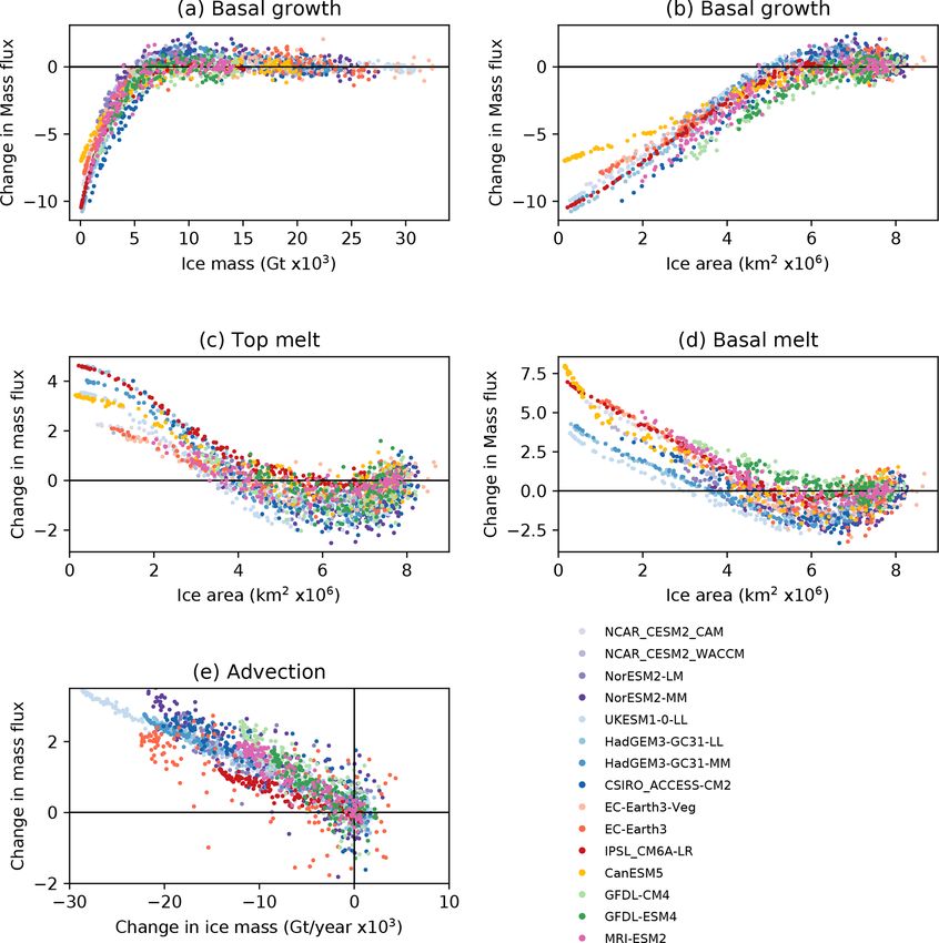
958                          A. Keen et al.: An inter-comparison of the mass budget of the Arctic sea ice in CMIP6 models

Figure 2. Evolution of (a) March (solid lines) and September (dash lines) ice area and (b) March ice mass for the CMIP6 models. Also shown
is (a) the mean and range for the HadISST1.2 (Rayner et al., 2003), HadISST.2.2 (Titchner and Rayner, 2014) and OSI-SAF (OSI-SAF, 2017)
observational datasets and (b) the PIOMAS reanalysis (Zhang and Rothrock, 2003) with uncertainty estimate (Schweiger et al., 2011).

in Fig. 1a, for the multi-model mean for the reference pe-             from the ocean and 25 % by melt at the ice surface (Fig. 4b).
riod 1960–1989. The black line shows the total amount of               The monthly maximum ice melt occurs in July, with both top
ice growth or loss each month, with net ice loss occurring             and basal melt peaking at this time, and the basal melt contin-
from May to September and net ice growth from October to               ues further into the late summer than the top melt (Fig. 4a).
April. Most of the increase in ice mass results from growth            Ice lost by advection out of the region accounts for 19 %
at the base of existing ice, which occurs between September            of the total (Fig. 4b), and this is likely to be dominated by
and May and represents 83 % of the total annual ice growth             loss through the Fram Strait. The advective ice loss occurs
(Fig. 4b). Frazil ice formation in open water accounts for             all year, and although it is greater during the winter than the
16 %, with the small remainder due to snow ice formation.              summer, the magnitude of the seasonal cycle is far smaller
Most of the ice loss occurs during the summer, with 52 % of            than that for either the top or basal melting (Fig. 4a).
the annual mean ice loss caused by basal melting due to heat

The Cryosphere, 15, 951–982, 2021                                                            https://doi.org/10.5194/tc-15-951-2021
A. Keen et al.: An inter-comparison of the mass budget of the Arctic sea ice in CMIP6 models                                   959

Figure 3. Evolution of annual-mean global-mean near-surface temperature for the CMIP6 models and the HadCRUT4 observational dataset
(Morice et al., 2012). Values are relative to the 1960–1989 mean in each case.

  In summary, for the 1960–1989 multi-model mean the                  – and a relatively symmetric seasonal cycle of total ice
dominant process causing ice growth is basal ice growth, fol-           growth and melt, centred around the maximum net ice
lowed by frazil ice formation, and the dominant processes               loss in July (not shown).
causing ice loss are basal melting, top melting and advection
out of our analysis region. For the remainder of the paper          However, there are also some notable differences between
we focus on these five main budget terms, as the remaining          the model budgets, which we describe below.
smaller terms do not contribute significantly to the mass bud-
                                                                    4.2.1   Ice growth
get for any of the models considered.
                                                                    The ratio between basal ice growth and frazil ice formation
4.2   Inter-comparison of the CMIP6 models                          varies significantly between the models. For example, for
                                                                    both the GFDL models almost all the annual ice growth is
Figures 5 and 6 show the annual means and seasonal cycles
                                                                    due to basal ice growth, whereas for the EC-Earth3 models
of the main budget terms for each individual model. Note
                                                                    73 % of the annual growth is due to basal growth and 25 %
that some models do not generate all the terms, and some
                                                                    to frazil ice formation. This different partitioning appears to
models have terms missing (see Table 1). It is striking to see
                                                                    relate to specific settings within the sea ice models, in par-
how similar the model budgets are, at least in a broad sense
                                                                    ticular the minimum thickness of frazil ice that is allowed to
(Fig. 5). For example, in all the models we see
                                                                    form. The lower the value of the minimum frazil ice thick-
                                                                    ness, the more quickly the frazil ice growth can transition to
  – more basal ice growth than frazil ice formation (Fig. 5);
                                                                    basal growth. This is discussed further in Sect. 5.
                                                                       If we consider the total amount of winter ice growth (here
  – virtually no ice growth between June and August                 taken as the sum of the frazil and basal growth terms), the
    (Fig. 6a and b);                                                spread in modelled values is 3.9 ×10³ Gt, compared to the
                                                                    larger range of 5.9 ×10³ Gt for the basal growth alone.
  – more basal melting than top melting (although                      The month in which the amount of frazil ice for-
    the difference is small for the UK models and                   mation peaks varies from October (UK models and
    CSIRO_ACCESS-CM2) (Fig. 5);                                     CSIRO_ACCESS-CM2) through November (EC-Earth3,
                                                                    EC-Earth3-Veg and CM6A-LR) to December for the remain-
  – a maximum in ice melting in July, with a peak in both           ing models (Fig. 6b). The amount of basal growth peaks in
    top melting and basal melting (Fig. 6c and d);                  December for most of the models (Fig. 6a).

  – basal melt continuing later into the autumn than top
    melting (Fig. 6c and d);

https://doi.org/10.5194/tc-15-951-2021                                                      The Cryosphere, 15, 951–982, 2021
960                          A. Keen et al.: An inter-comparison of the mass budget of the Arctic sea ice in CMIP6 models

                                                                     the models with the most top melting overall. Some mod-
                                                                     els have a fairly symmetrical peak in basal melting (for ex-
                                                                     ample the EC-Earth3 models and also the NCC_NorESM2-
                                                                     LM model), whereas some have a more pronounced “tail”
                                                                     of melt further into autumn (for example MRI_ESM2.0,
                                                                     NCAR_CESM2_WACCM) (Fig. 6d).

                                                                     4.2.3    Ice advection

                                                                     All the models for which we have the dynamics term show a
                                                                     net advection of ice out of the analysis region (Fig. 5). This is
                                                                     dominated by export through the Fram Strait. The net ice loss
                                                                     by advection varies from 1.2 ×10³ to 3.7 ×10³ Gt per year
                                                                     between the models and comprises between 9 % and 30 % of
                                                                     the total annual ice loss. There is no strong agreement be-
                                                                     tween models as to how this export varies during the year
                                                                     (Fig. 6e). Five of these 13 models have a minimum advective
                                                                     ice loss in August, but overall there is considerable variabil-
                                                                     ity between the models in terms of the amount and timing of
                                                                     the annual ice export.

                                                                     5     Understanding differences between the CMIP6
                                                                           models

                                                                     Having described the similarities and differences in CMIP6
                                                                     model ice budgets for the reference period 1960–1989, we
                                                                     now explore the extent to which these budget differences can
Figure 4. Components of the Arctic sea ice mass budget for the       be related to differences in model formulation and ice state.
multi-model mean. Values are summed over the region shown in         The sea ice mass budget in climate models is influenced by
Fig. 1, for the period 1960–1989. For each budget component, val-    both the sea ice physics and also the interaction with the at-
ues are calculated by averaging the ensemble mean for each model     mosphere and the ocean, meaning it can be difficult to isolate
with a non-zero value of the component. (a) Seasonal cycle of
                                                                     the impact of, say, a particular parametrization when inter-
monthly mean values; (b) annual mean values. The shaded regions
show ±1 standard deviation in the modelled values. Percentages are
                                                                     comparing different models. Hence to aid our understanding,
relative to the total annual mass of ice growth or loss.             we also draw on information from a set of ocean–ice experi-
                                                                     ments, where the atmospheric forcing and sea ice physics are
                                                                     varied independently. In this section, we also try to identify
                                                                     the influence of the sea ice model physics on the different
4.2.2   Ice melt                                                     mass budget terms.

The relative amount of basal and top melting also varies             5.1     Description of the forced ocean–ice experiments
considerably between the models, with top melting rang-
ing from 28 % to 91 % of the amount of basal melt. The               We consider three integrations using a forced ocean–ice
UK models (HadGEM3-GC31-LL, HadGEM3-GC31-MM                          model with the same sea ice and ocean components as
and UKESM1-0-LL) together with CSIRO-ACCESS-CM2                      the HadGEM3-GC31-LL model. The advantage of using a
have almost as much ice lost by top melting as by basal              forced model is that we can look at the impact of changing
melt, in contrast to the other models which have consider-           sea ice physics or atmospheric forcing independently (Ta-
ably more basal melt than top melt (Fig. 5). The models              ble 3). The main disadvantage is that it does not represent
agree very well on the amount of top melting late in the sea-        atmosphere–sea ice and atmosphere–ocean feedbacks. It is
son (August–September). However, the onset of melt (May–             noteworthy that the default forced simulation differs strongly
June) and peak in melting in July show much more variabil-           from the HadGEM3-GC31-LL simulation despite the same
ity (Fig. 6c). This is consistent with the former being mainly       sea ice settings (Fig. 7). In contrast to HadGEM3-GC31-LL,
related to the solar zenith angle, whereas the latter is also        sea ice mass and area are smaller in the forced simulation
related to other factors like ice and snow surface tempera-          than in PIOMAS and HadISST and OSI-SAF respectively.
ture and surface albedo. Seven out of the 15 models have             The stronger top and basal melt in the forced simulation
more top melting than basal melting in July, and these are           (Fig. 8c and d) leads to a stronger annual cycle and smaller

The Cryosphere, 15, 951–982, 2021                                                         https://doi.org/10.5194/tc-15-951-2021
A. Keen et al.: An inter-comparison of the mass budget of the Arctic sea ice in CMIP6 models 961 Figure 5. Main components of the annual mean Arctic sea ice mass budget for each model. Values are summed over the region shown in Fig. 1, for the period 1960–1989. The grey bars show the multi-model mean for each term for the same period. https://doi.org/10.5194/tc-15-951-2021 The Cryosphere, 15, 951–982, 2021
962                          A. Keen et al.: An inter-comparison of the mass budget of the Arctic sea ice in CMIP6 models

Figure 6. Seasonal cycles of the main components of the Arctic sea ice mass budget. Values are summed over the region shown in Fig. 1, for
the period 1960–1989.

sea ice area during summer (Fig. 7a). This suggests that the           and slightly increases the basal growth (Fig. 8a), which in
interaction with the atmosphere is responsible for the overes-         turn increases sea ice area and mass (Fig. 7). The new set-
timation of sea ice mass in HadGEM3-GC31-LL.                           tings include the elastic–anisotropic–plastic (EAP) rheology
   Applying changes to the sea ice physics which results in            (Tsamados et al., 2013), the bubbly conductivity formulation
improved sea ice evolution in a stand-alone sea ice simula-            from Pringle et al. (2007), a simple scheme to account for the
tion (Schroeder et al., 2019) reduces the basal melt (Fig. 8d)         loss of drifting snow, increased longwave emissivity of sea

The Cryosphere, 15, 951–982, 2021                                                            https://doi.org/10.5194/tc-15-951-2021
A. Keen et al.: An inter-comparison of the mass budget of the Arctic sea ice in CMIP6 models                                     963

Figure 7. Seasonal cycles of (a) ice area and (b) ice volume for the period 1990–2009, for the forced ocean–ice runs (Table 3), plus
HadGEM3-GC31-LL and the other CMIP6 models. Where more than one model integration is available, the values are ensemble means.
Also shown are data for the same periods for (a) the HadISST1.2 (Rayner et al., 2003), HadISST.2.2 (Titchner and Rayner, 2014) and
OSI-SAF (OSI-SAF, 2017) observational datasets and (b) PIOMAS reanalysis (Zhang and Rothrock, 2003) for the same period.

ice from 0.95 to 0.976, and a reduction in the maximum melt-        the full potential variations in sea ice physics. A similar effect
water added to melt ponds (rfracmax) from 100 % to 50 %             was found by Massonnet et al. (2018), who showed that us-
(Schroeder et al., 2019). These changes do not bracket the          ing the simplest Semtner zero-layer model and varying only
whole range of physics seen in the CMIP6 models, but the            one parameter (ice albedo) could explain a great fraction of
forced experiments do include physics not used in any of the        CMIP5 model spread.
CMIP6 models included in this paper (the EAP rheology and              Replacing the CORE forcing which is based on NCEP re-
bubbly conductivity). The differences regarding the sea ice         analysis (Large and Yeager, 2009) with the Drakkar forcing
area and mass, and the basal melting, are striking given we         set (DFS) based on ERA-Interim reanalysis (Dussin et al.,
apply the same sea ice model, and the changes do not bracket        2016) increases the top melt (Fig. 8c) and decreases the basal

https://doi.org/10.5194/tc-15-951-2021                                                       The Cryosphere, 15, 951–982, 2021
964                          A. Keen et al.: An inter-comparison of the mass budget of the Arctic sea ice in CMIP6 models

Figure 8. Seasonal cycles of the main components of the Arctic sea ice mass budget. Values are summed over the region shown in Fig. 1, for
the period 1960–1989, for the forced ocean–ice runs (Table 3), plus HadGEM3-GC31-LL and the other CMIP6 models.

melt (Fig. 8a), resulting in higher sea ice area and mass. In-         CMIP6 models than in these two forcing datasets, which are
terestingly, differences between the CORE- and DFS-forced              both based on re-analyses. The CMIP6 models also represent
experiments in late summer suggest that the winds and large-           the two-way atmosphere–ice interactions, which the forced
scale atmospheric circulation are having a larger impact than          models do not. Looking at the different components of the
sea ice physics on sea ice dynamics (Fig. 8e). It is likely            mass budget, these three forced experiments can nearly ex-
that there is more diversity in the atmospheric forcing in the         plain the full CMIP6 model spread for basal sea ice melt al-

The Cryosphere, 15, 951–982, 2021                                                            https://doi.org/10.5194/tc-15-951-2021
A. Keen et al.: An inter-comparison of the mass budget of the Arctic sea ice in CMIP6 models                                  965

though only a small part of the differences in top melting and    frazil ice. The GFDL-CM4 and GFDL-ESM4 models with
sea ice growth. These experiments confirm that both the sea       the SIS2 sea ice component have no minimum thickness,
ice physics and the atmospheric forcing are key factors in        which means these models can grow arbitrarily thin frazil ice.
determining what the ice state and mass budget look like and      This means the frazil ice can quickly transition to congelation
can produce changes of comparable magnitude.                      growth, and these models form less than 0.04 ×10³ Gt/year
                                                                  of frazil ice. Of the remaining models, those that can form
5.2     Individual budget terms in the CMIP6 models               thicker frazil ice tend to form more frazil ice and correspond-
                                                                  ingly less ice via basal growth. There are four models us-
We now consider each of the mass budget terms in turn to see      ing LIM3 with a minimum frazil ice thickness of 10 cm, and
to what extent we can find factors that might explain the dif-    these form between 2.5 and 3.5 ×10³ Gt/year of frazil ice
ferences between the CMIP6 models. When looking at differ-        (Fig. 9b). The remaining models have a minimum frazil ice
ences in model formulation, we have focussed on the physics       thickness of 5 cm, and six out of eight of them form less ice
and parameter choices made within each sea ice component.         than the models with a 10 cm minimum thickness. While it is
The sea ice models used here share a number of key param-         not unexpected that the minimum frazil ice thickness affects
eterizations and often provide a choice of different schemes      the amount formed within a particular model, it is notable
to choose from. For example, this study includes models us-       that this relationship is seen so strongly across the majority
ing Community Ice CodE (CICE), Sea Ice Simulator (SIS)            of models considered here, despite all the other differences in
and Louvain-la-Neuve sea ice model (LIM) sea ice compo-           model formulation. The sea ice component affects the month
nents that all use the BL99 (Bitz and Lipscomb, 1999) ther-       in which the frazil ice formation peaks (Fig. 6b): models us-
modynamic scheme, while there is another that uses CICE           ing CICEb have a maximum in October those using LIM3 in
with the T13 (Turner et al., 2013) thermodynamics. The sea        November, and those using CICEa in December.
ice models used in the CMIP6 models considered here can              The B20 study found that the T13 thermodynamic scheme
be grouped according to a number of key model parameter-          tends to produce more frazil ice than BL99; however this dif-
izations and settings (Table 4), and for each budget compo-       ference is not evident in the models considered here. Another
nent, we consider its relationship with these (Fig. 9), as well   finding from B20 is that model configurations with larger ex-
as the ice state (March and September ice area, and annual        tents tend to have more frazil formation, as the biggest differ-
mean ice mass) and atmospheric near-surface temperature           ences are seen in the marginal ice area. Here, while the four
(not shown). Note that the mean values of ice state and at-       models with the largest March ice area do form relatively
mospheric temperature discussed here are calculated for the       large amounts of frazil ice, there is not a strong correlation
reference period 1960–1989 and so (for ice state) do not ex-      when all the models are considered, likely due to the areal
actly match the data as shown in Fig. 1.                          domain considered in this study.
5.2.1    Basal growth
                                                                  5.2.3   Top melt
The two factors most influencing the amount of basal growth
in the models considered here are the thermodynamic scheme        We have found links between the amount of top melt-
and the melt pond formulation. The models using CICEb,            ing and the melt pond formulation, the thermodynamic
LIM3 and SIS2 use the BL99 thermodynamic scheme, and              scheme, the treatment of incoming shortwave radiation and
seven out of nine of these have more basal growth than the        the global mean near-surface temperature. Eight of the 15
four CICEa models using T13. This is consistent with sen-         CMIP6 models have a relatively small amount of top melt-
sitivity experiments using the CESM2_CAM model (Bailey            ing (Fig. 9c), melting between 2.1 and 2.5 ×10³ Gt/year
et al., 2020) (B20), which found more basal growth with the       of ice. The remaining seven models melt between 3.5 and
BL99 scheme than T13. The eight models that use CICE all          4.9 ×10³ Gt/year. Of the models with prognostic melt pond
have prognostic melt ponds. Those using CICE 5.1.2 GSI8.1         schemes, those models using H13 (CICEa) have less top
(CICEb) have the F12 scheme (Flocco et al., 2012) and have        melting than those using F12 (CICEb). For models with a
more basal growth than those using CICE5.1.2 (CICEa) with         parameterized representation of melt ponds there is no clear
the H13 melt pond scheme (Hunke et al., 2013) (Fig. 9a). The      separation in the amount of top melt. A unique feature of the
models with parameterized melt ponds show a wide range of         models using CICEb compared to the other CMIP6 models
values of basal growth. We have not found a relationship be-      considered here is that they do not allow any of the incom-
tween the amount of basal growth and the ice state or global      ing shortwave radiation to penetrate through the sea ice to the
atmospheric temperature.                                          ocean. Development experiments using an updated version of
                                                                  the UK model show that there is a large reduction in top melt
5.2.2    Frazil ice formation                                     (around 20 %) when the penetration of shortwave radiation is
                                                                  included (Blockley, private communication), consistent with
The main factor affecting the amount of frazil ice formed by      the relatively high amount of top melting seen here in the
each model is the value chosen for the minimum thickness of       models without this feature.

https://doi.org/10.5194/tc-15-951-2021                                                    The Cryosphere, 15, 951–982, 2021
966 A. Keen et al.: An inter-comparison of the mass budget of the Arctic sea ice in CMIP6 models
Table 4. Selected features of the sea ice components used by the CMIP6 models. References for each scheme are provided in Table 2.
Sea ice configuration Thermodynamics Melt ponds Minimum frazil thickness
CICE 5.1.2 (CICEa) T13 Prognostic H13 5 cm
CICE5.1.2 (GSI8.1) (CICEb) BL99 Prognostic F12 5 cm
LIM3 BL99 Prescribed albedo reduction 10 cm
LIM2 Zero layer Parameterized 5 cm
SIS2 BL99 Parameterized None
MRI.COM 4.4 (COM4) MK89 Parameterized –
Figure 9. Main components of the annual mean Arctic sea ice mass budget for each model, for the reference period 1960–1989. Values are
grouped by key features of the sea ice model as summarized in Table 4 and where CICEa is CICE 5.1.2, CICEb is CICE 5.1.2 (GSI8.1) and
COM4 is MRI_COM4.4.
The four models using CICEa with the T13 thermody- lationship with September ice area or annual ice mass. The
namic scheme have a relatively small amount of top melt. majority of the models with less top melting (seven out of the
The B20 study found more top melting with the BL99 eight) have a relatively high global near-surface temperature.
scheme than with the T13 scheme. Here we find that a ma-
jority of the models using BL99 (six out of nine) have more 5.2.4 Basal melt
top melt than the models using T13, with the remaining three
having a similar amount of melt to the T13 models. Six out
Models with a lower September ice area tend to have more
of the seven models with the larger amount of top melting
annual basal melt. This would be consistent with those mod-
have relatively low March ice area: there is no obvious re-
els having a greater potential for atmospheric heating of
The Cryosphere, 15, 951–982, 2021 https://doi.org/10.5194/tc-15-951-2021A. Keen et al.: An inter-comparison of the mass budget of the Arctic sea ice in CMIP6 models 967
the upper ocean, due to the lower ice cover. Models with melt and top melt. The F12 scheme tends to be associated
a smaller annual mass of ice also tend to have more basal with more basal growth and top melt but less basal melt than
melt. These findings are consistent with the results from the H13. One notable result is that the amount of frazil ice forma-
forced ocean–ice experiments. The amount of basal melt will tion is strongly dependant on the value chosen for the mini-
also be affected by the ocean temperature and heat budget of mum frazil ice thickness, despite all the other differences in
the upper ocean, but an analysis of these factors is outside model formulation.
the scope of this study. The models with parameterized melt The thermodynamic scheme used is related to the amount
ponds tend to have more basal melt than those using CICE of basal growth and top melt, with models using the BL99
with prognostic melt ponds (Fig. 9d). For those models using scheme having more basal growth and top melt than those
prognostic schemes, models using H13 (CICEa) tend to have using T13. This result is consistent with that of Bailey et
more basal melt than those using F12 (CICEb), although it al. (2020), who studied the impact of the BL99 and T13
is not a very marked difference. The two models using the thermodynamic schemes within a single climate model. This
zero layer and MK89 thermodynamic schemes (LIM2 and study also found that the T13 thermodynamic scheme results
COM4.4) have more basal melt than the other models. The in more frazil ice formation and basal melt than BL99. We
B20 study found more basal melt with the BL99 thermody- cannot detect this amongst the CMIP6 models, possibly be-
namic scheme than with T13, but this is not evident in the cause of the many other differences in model formulation.
CMIP6 models. Models using the BL99 scheme (CICEb, Models using the MetUM and NorCAM6 atmospheric
LIM3 and SIS2) have a relatively wide range of basal melt component tend to have more dynamic ice loss than the
(from 4.5 to 7.58 ×10³ Gt/year) compared to those using CI- other models, which is potentially consistent with the finding
CEa with T13 (6.1 to 6.9 ×10³ Gt/year), but there is no clear from the forced experiments that winds and large-scale atmo-
separation in the amount of basal melt between models using spheric circulation are important in determining the amount
these two thermodynamic schemes. of dynamic ice loss. These models also have higher ice mass
In Sect. 4.2 it was noted that the majority of models have than most of the other models, so for the same sea ice drift
notably more basal melt than top melt (Fig. 5). The excep- they will export more sea ice mass from the domain. We
tions are the UK models and CSIRO_ACCESS-CM2, where have not found any other clear links between the mass bud-
the difference is much smaller. This is likely to be due to get components and the atmospheric model used. This is
the lack of penetrating solar radiation mentioned above, al- perhaps surprising given the results from the forced experi-
though these models do also share the same sea ice (CICEb) ments. However, it may be that the internal atmospheric vari-
and atmosphere (MetUM) components, so there are poten- ability masks this within the CMIP6 model experiments. It
tially other factors which could also be responsible. is also worth noting that all the models using the F12 melt
pond scheme have a common atmospheric model (MetUM),
5.2.5 Ice advection so this may also be a factor affecting the top melt, basal melt
and basal growth.
Models with a larger annual mean mass of ice tend to lose In summary, we have found a number of relationships be-
more ice each year by advection out of the analysis region. tween model formulation and components of the ice budget
There is also a similar relationship with September ice area that hold for all or most of the CMIP6 models considered
and to a lesser extent with March ice area. This is perhaps not here.
surprising – if there is more ice in the Arctic basin there is
more available to be transported out. There is some evidence
that the atmospheric component plays a role: for example, the 6 Projections of the sea ice mass budget during the 21st
models using MetUM and NorCAM6 atmospheres have the century
most advective ice loss (Fig. 9e). Apart from that, we have
found no clear link between the ice loss by advection and the We now consider how the mass budget of the CMIP6 mod-
model formulation. This is consistent with the findings from els changes during the 21st century as the ice cover and mass
the forced experiments, where winds and large-scale atmo- declines and the environment warms. We first look at the evo-
spheric circulation have a larger impact than sea ice physics lution of the budget terms for the multi-model mean, and then
on sea ice dynamics. we consider the differences between individual models.
5.2.6 Summary 6.1 Multi-model mean
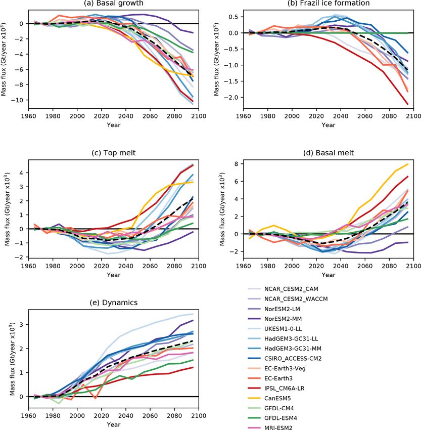
We have identified a number of potential links between The magnitude of each budget term tends to decrease with
model physics and ice state and the major components of time, consistent with the reducing mass of the ice (Fig. 10a).
the ice mass budget amongst the CMIP6 models for the ref- Throughout the time period considered here there is a greater
erence period 1960–1989. For models with prognostic melt mass of ice formed by basal growth than by frazil ice forma-
ponds, the choice of scheme may affect basal growth, basal tion and more basal than top melt. The amount of ice lost
https://doi.org/10.5194/tc-15-951-2021 The Cryosphere, 15, 951–982, 2021You can also read