And attention based model for

Clustering and attention based model for
intelligent trading

 ,
 Mimansa Rana, Nanxiang Mao Ming Ao, Xiaohui Wu, Poning Liang and Matloob Khushi
 The School of Computer Science, The University of Sydney

 ABSTRACT

The foreign exchange market has taken an important role in the global financial
market. While foreign exchange trading brings high-yield opportunities to investors,
it also brings certain risks. Since the establishment of the foreign exchange market in
the 20th century, foreign exchange rate forecasting has become a hot issue studied by
scholars from all over the world. Due to the complexity and number of factors affecting
the foreign exchange market, technical analysis cannot respond to administrative
intervention or unexpected events. Our team chose several pairs of foreign currency
historical data and derived technical indicators from 2005 to 2021 as the dataset and
established different machine learning models for event driven price prediction for
oversold scenario.

 i

1. INTRODUCTION
With development of the economy and improvement of people's living standards, the
consciousness of investment gradually appears in the minds of the public. The
foreign exchange market has far surpassed other markets such as stocks and futures,
becoming the largest financial market in the world [1]. The rapid growth in the size
of the foreign exchange market has brought high profits and high risks at the same
time. So it becomes important to be able to make effective predictions on the trend of
foreign exchange prices. Foreign exchange markets change irregularly over time.
Under fast changing international pattern and corresponding policies, there are many
factors affecting the exchange rate fluctuations. The artificial trading is easy to
produce negative emotions and difficult to observe the market situations at all times.
On this basis, we adopt machine learning/deep learning models to improve predictive
accuracy in foreign exchange market using basic price information as well as derived
technical indicators. And eventually, the prediction model can be used by a wide
range of stakeholders including banks and hedge funds to diversify their trading
strategies as well generate stable profits over time.

2. RELATED LITERATURE
2.1 Technical indicators

Technical indicators are often used to determine trading strategies within the Forex
Market as they can be used to understand trends and signal upcoming changes in
market conditions. Below are some indicators that we have found being commonly
used during our research.

2.1.1 Relative Strength Indicator (RSI)
RSI (relative strength indicator) is used to determine overbought or oversold
conditions in the market. It is calculated using the below formula

 100
 = 100 − (1)
 1 + 
 
 = (2)
 

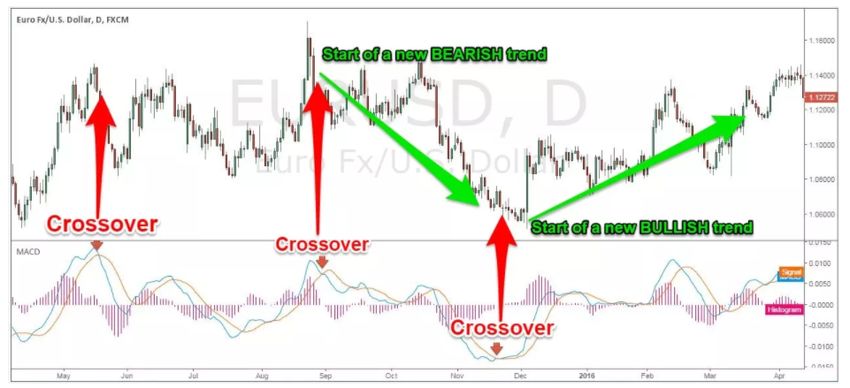
RSI is an oscillator indicator and its value lies between 0 and 100. A value of < 30
indicates that oversold market conditions while an RSI value of >(70-80) indicates
overbought market conditions. Oversold market conditions usually means that there is
an increase in the likelihood of price going up and an opportunity to buy. Overbought
market conditions usually indicate the increase in likelihood of the price going down
and an opportunity to sell.

 Figure 1 [2]

2.1.2 Simple Moving Average (SMA), Exponential Moving Average (EMA),
 MACD (Moving Average Convergence Divergence)
MACD is a useful indicator to compare short term and long term price trends, which
help to determine buy or sell points. In order to calculate MACD we first calculate
Simple Moving Average (SMA) and Exponential Moving Average (EMA).

SMA is the average of a range of prices divided by the number of periods in the range.

EMA is similar to SMA except that the more recent prices are given a higher weight
during the calculation of the average.

 = ( 12 )– ( 26 ) (3)

The MACD values are usually plotted on the same graph as the 9 day SMA of the
forex values (the 9 day SMA line is usually called Signal Line) . The movement of
MACD line relative to the Signal line determines if the market is Bullish or Bearish

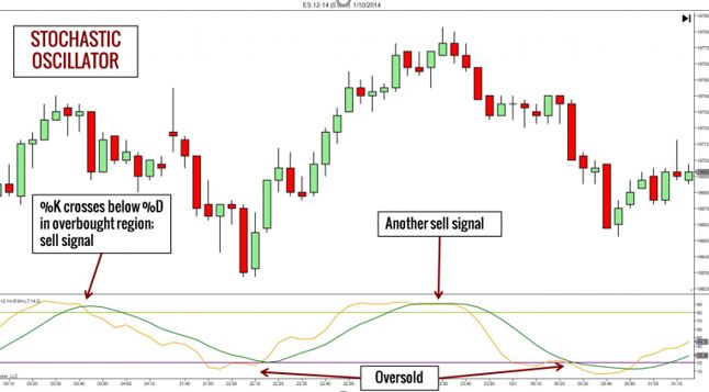
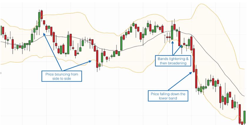
and can be useful to determine if the trader should look for a long or short position.

 Figure 2 [3]

2.1.3 Bollinger Bands
Bollinger Bands are a set of trendlines or bands plotted for a SMA plus/minus 1
standard deviation and 2 standard deviations from SMA. The area represented by 1 SD
from SMA on either side represents the Average Band, whereas the area represented
by the lines 2 SDs away from SMA indicate the Higher and Lower bands.
Approximately 90% of the price movement occurs between the 2 bands (upper and
lower), so any changes in price outside the bands could be a significant event. A
narrowing or squeezing of the band itself is also seen as a period of low volatility and
could signal future increase in volatility.

 Figure 3 [4]

2.1.4 KD – stochastic indicator
Stochastic Oscillaor (%K) is a momentum indicator that is often used to determine
signals to a movement in price before it occurs or trend reversals. When depicted on a
graph it is usually drawn with %D line which is the 3 period SMA of %K.

% K is calculated using the following formula:

 − 
 % = 100 E G (4)
 − 

Where

 C is current closing price.

 Hn, Ln are the highest and lowest prices respectively in the previous n trading
sessions.

The relative movement of the 2 lines (%K and %D) and especially the points when
they cross over can be used to predict trend reversals or overbought/oversold
conditions.

 Figure 4 [5]

2.1.5 DMI - Directional movement index
Directional movement index is used to identify what direction the asset price is
moving. It compares prior high and lows and draw two lines: the positive directional
movement line (+DI) and a negative directional movement line (-DI). When +DI is
above -DI meaning there is more upward pressure than downward pressure on price.

 (5)

Where:

2.1.6 Concealing Baby Swallow Candlestick pattern
Concealing Baby Swallow Candlestick pattern is made up of four candlesticks. First
candlestick: a marubozu candlestick with a bearish body. Second candlestick opens
within the prior one’s body and close below prior closing price. The third candlestick
has long upper shadow and no lower shadow. It opens below prior closing price and
upper shadow enters the prior candlestick’s body. The fourth one is a tall candlestick
with its body covers the pervious candlestick’s body and shadows.

 (28)

2.1.7 Pattern: Oversold/Overbought
There are two types of oversold scenarios: fundamentally oversold and technically
oversold. Fundamentally oversold is when an asset is trading below their true value
(overbought is the opposite to oversold). This could be because people have a
negative outlook for the asset or any underlying risks that prevent people from
buying it. One of popular indicators for a fundamentally oversold is P/E ratio. For
technical oversold, it can be defined as a period of time when there has been some
significant and consistent downward movement in price without any bounce. And
in a technical oversold condition we only consider technical indicators such as RSI
and stochastic indicators: an asset is considered to be technically oversold when its
14 periods RSI is equal to or below 30 and overbought when the RSI is equal to or
above 80.

2.2 Literature Review

The field of machine learning and artificial intelligence is evolving very rapidly and
there are new models and architectures being proposed every year that can outperform
existing benchmarks. Financial markets specifically are of great interest to researchers,
industry and academics as there are significant financial gains at stake. However the
challenge with financial market data is that it is noisy, volatile and often unpredictable
and there are a few papers we have come across which uses techniques such as PCA[6],
wavelet denoising [7],[8], [50] or bagging [9]. [44] employs the use of feature
selection to improve performance of stock price prediction.

Several papers deploy architectures based on traditional machine learning models
combined with deep learning or neural network architectures to make predictions on
future price of stock or forex values based on historical data. [10] proposes a 2-stage
approach to predict values of stock market index, a Support Vector Regressor (SVR)
based data preparation layer, followed by combinations of Artificial Neural Network
(ANN), Random Forest (RF) and SVR. [11] uses a multi-level architecture stacked
made up of common machine learning algorithms such as SVM, Random Forest,
Dense Layer NN, Naïve Bayes and Bayesian autoregressive trees (BART) and
aggregates the scores obtained using a stacked generalisation mechanism. [12] uses
Genetic Algorithm along with Neural Network to provide a Forex Trading system.
[26] splits a whole time-series data into equal length sub-sequence and use k-means to
allocate instances into different groups before applying a LSTM model for training
and prediction. [48] uses genetic algorithm to for forex price prediction.

[46] performs a review of the methods used in research papers in the field of forex and
stock price prediction and concludes that in recent years the use of deep learning
models has increased as these methods provide better results and performance.

Several papers use architectures with neural network-based models that make
predictions based on sequential input data (sequence2sequence models) such as
[13] which uses an LSTM network to model historical data in order to predict future
price movement of stocks to achieve 20% return. LSTM is combined with GRU in
[14] to make prediction on FX rates, and the model outperforms a model based on
GRU or LSTM alone. [15] uses an LSTM-CNN network to predict future stock price,
achieving an annualised return of 33.9% vs 13.5% benchmark. [45] also uses event
driven LSTM to predict forex price.

Long short-term memory model has been shown to be very effective in many time-
series prediction problems, this model is popular to be used in price prediction in stock
market and forex recent years. Since in the forex market, fundamental and technical
analysis are two main techniques. [20] used LSTM to forecast directional movement
of forex data with technical and macroeconomic indicators. They utilized two different
datasets which are macroeconomic data and technical indicator data to train LSTM
model, this experiment was found to be quite successful with real world data. For the
same data, there are different representations which means it can have various features.
[21] developed a long short-term memory-convolutional neural network (LSTM-
CNN) model that it can learn different features from a same data, namely, it can
combine the features of stock time series and stock chart images to forecast the stock
prices. In their experiment, the hybrid model outperforms the single models (CNN and
LSTM) with SPDR S&P 500 ETF data. Also, they found that the candlestick chart is
the best chart for this hybrid model to forecast stock prices. This research has proved
that the combination of neural network models can efficiently reduce the prediction
error.

Attention based mechanisms and transformers have gained popularity in the last 1-2
years and they tend to be the State-of-the-Art standard at the moment [16]. These
architectures are used in many fields of research from NLP to computer vision. An
attention-based LSTM model is used to predict stock price in [18]. The prediction is
based on both live Twitter data (using NLP to do sentiment analysis) and technical
indicators to achieve an MAE of 0.484 and MSE of 0.627. [19] also uses an attention-
based LSTM model to predict stock price. With the help of attention layer, the model
is able to learn what part of historical data it needs to put more focus on and it has
achieved a better performance than LSTM. The model has achieved a MAPE of
0.00550 vs 0.00838 using LSTM and 0.01863 using ARIMA. [8] proposes first de-
noise data (i.e. stock price and volume) using wavelet in order to effectively separate
useful signal from noise, and then feed data into an attention based LSTM model that
has achieved a MSE of 0.1176 vs 0.1409 from GRU and 0.1839 from LSTM. [47] uses
a combination of reinforcement learning and attention with transformer model to make
predictions on stock data. Transformer architecture is also used in [43], not just for
price prediction but for text mining to create a financial domain specific pretrained
sentiment analysis model.

Reinforcement learning includes many different types of algorithms, and these
algorithms can make trained models achieve different performances. From conclusion
from paper written by Thomas G. Fischer [22], the actor-only approach has a better
performance than other methods, however, the critic-only approach are used more
widely. And the performance of the critic-actor approach is poor due to the
unpreventable correlation generated by the critic-actor approach itself. Besides, the
indicators used in the actor-only approach is not decisive since the model can find the
policy and inner relation by itself. One of the papers published by Dempster [23] used
14 indicators but they did not help in improving the performance. [49] reviews and
critiques existing work that is using reinforcement learning in financial markets.

Stacked autoencoder (SAE) has been widely used in the prediction of time series data
due to its excellent performance in depth extraction of data set features
[30,31,32,33,34]. The researchers also provided an answer to the question of whether
the SAE approach can be applied to financial market forecasting. In 2016, the
researchers proposed a prediction model that combined SAE and SVR and made
predictions on 28 currency pairs datasets. The ANN and SVR models are used as the
benchmark models, and the results show that this model has better performance than
ANN and SVR to some extent. For example, the model is 6 times better than the ANN
model in MSE [33]. Bao et al. used wavelet transforms (WT), SAE, and LSTM to
predict stock prices and compared them with WT+LSTM and LSTM. It is proved that
the SAE method can effectively improve the accuracy and profitability of the model
prediction [34].

3. RESEARCH/PROJECT PROBLEMS
In modern financial market, trading in commodities/shares/foreign currencies/other
financial instruments have been heavily adopted with latest technologies. From fast
evolving telecommunication technologies to more globalised banking systems, it helps
to grow the size of the financial market exponentially. In 2021, average daily turnover
for foreign exchange market is over $6.6 trillion [24] vs 2020 USA annual GDP of
20.93 trillion [25]. As a result, people are always looking for new trading strategies
using latest technology in order to make profits. Algorithm trading is among one of
the most popular area which can be traced back to 1970’s when it was first introduced

as “designated order turnaround system” by New York Exchange. Nowadays,
algorithm trading has been dominating the space from high frequency trading to
portfolio management.

Our project problem is whether we can use the latest deep learning algorithms to
improve predictive accuracy in foreign exchange market based on basic price
information as well as derived technical indicators. Furthermore, with the help of the
deep learning algorithm whether we can develop a profitable trading strategy and also
minimise downside risks at the same time.

3.1 Research/Project Aims & Objectives

The goal of this project is to adopt various machine learning/deep learning models to
make accurate predictions on foreign exchange price movement. Because there are a
lot of factors will impact FX market such as political or economic ones that makes it
very difficult to predict every move solely based on technical indicators. Therefore,
we want to do event driven price predictions on any oversold conditions only.
Furthermore, we will also modify some latest deep learning algorithm to ensure its
adoption of the task yield even better result.

3.2 Research/Project Questions

To achieve a desirable outcome or provide some meaningful insight for other people
who will look into this area, there are a few important questions need to answer:

 o What data or technical indicators are important for the prediction?

 o What is the ideal sequence length of timestep regarding input data? This will
 also depend on what algorithm we use since more recent ones (such as
 attention or transformer) have much better memorability.

 o How are hyper parameters going to impact our models’ performance?

 o Considering the achievements of different machine learning models in time
 series forecasting, what type of algorithm are more suitable for this task?

 o For some algorithms, what types of data pre-processing is required (i.e. PCA,
 data cleaning and etc)?

o How do we evaluate outcome of our project (i.e. whether we can prove a
 positive return based on the prediction made by our models or using some
 traditional metric such as MSE or MAE to measure forecast accuracy)?

3.3 Research/Project Scope

The main work of the project was divided into three parts. First, data pre-processing
and feature engineering are performed to obtain technical indicators as data features.
Then different machine learning models are built to compare their performances. We
also try to ensure that each model is to achieve its best possible performance through
hyper-parameter tuning.

Data used: several pairs of foreign currency historical data dated from 2005 to 2021
will be used for training and testing for the project.

Success Criteria:

l All team members contribute evenly to our project goal on weekly basis.

l Each person to make significant contribution to developing/implementing
 machine learning model and fine tuning it in order to optimise its performance.

l Implement models with novel ideas along with outstanding prediction
 performance.

l The model can be applied to real-world forex forecasting problems with
 acceptable results.

Potential Risks:

l Timing risk – depending on amount of workload and everyone’s capacity there
 are risks of delivering certain goals/milestones in lateness.

l Technical risk – due to complexity of some models it might be difficult to
 construct or exceed our current abilities which result in fail in implementation.

l Performance risk - there are chances that our models are unable to generate out-
 performing results.

4. METHODOLOGIES
4.1 Methods

4.1.1 Clustering + Attention:

Step1 Feature selection:

In total there are more than 130 technical indicators available that can be used as input
features of our model. To select the best features, we write a loop function which takes
each feature and combine with “Open” and “Close” price to predict high price of next
60 mins. Each feature is trained for 35 epochs and then average loss of the final 10
epochs are calculated and used to rank its importance. We then choose the top 4 most
important features along with ‘Open” and “Close” as our input features.

Step 2 Clustering:

Clustering is one of the most common machine learning methods to identify subgroups
in a dataset so that data in the same subgroups have certain degree of similarities while
those in different groups tend to have different patterns. In other words, it helps to
discover homogeneous subgroups within a dataset such that data within each cluster
are as similar as possible and at the same time keep each cluster as far (different) as
possible. In the task of foreign exchange prediction, we use clustering to divide our
training dataset into various clusters based on input features (technical indicators) such
that data with similar price patterns can be grouped together. As a result, we expect it
to segregate instances that are heavily driven by news or any other non-technical
factors from those can be solely predictable based on technical indicators. The main
clustering method we used is Kmeans: the algorithm randomly initializes k number of
centroids and assign each data point to the cluster of the closest centroid. Then for each
cluster, it re-calculates centroids by finding mean of the data points previously
assigned. The algorithm repeats the above steps by re-assigning all the datapoint to the
closest centroid and re-calculating the centroid again and again until there are no
further updates/changes to all the centroids. Please see below objective function for
Kmeans. Please note that Wik = 1 if data point x belongs to cluster k, otherwise wik =
0.

(29)

Step 3 Prediction:

We apply BiLSTM with attention to each of the cluster from step 1 and make
prediction for the next 60 mins high. Dot product attention was used to calculate
attention score based on final hidden state and output states of the BiLSTM. By using
attention, the model can eliminate locality bias since it can attend to any information
from any time step using the attention layer. There are four major steps involved in
attention layer. First, to calculate dot product between last hidden state and output state
of the BiLSTM. Secondly, to work out probability distribution based on the output
from above using softmax function. Thirdly, to use the probability distribution from
previous step to calculate weighted sum of the output states. Lastly, the weight sum
and last hidden state will be passed through another RNN before concatenating its
output to last hidden states and passing it through a linear layer. Please see below figure
4.1.1.1 for the architecture of the attention model.

 Fig 4.1.1.1

4.1.2 Transformer Multi head attention

The components of transformer architecture we use in our model are as per below:

• Multi – head Self - attention

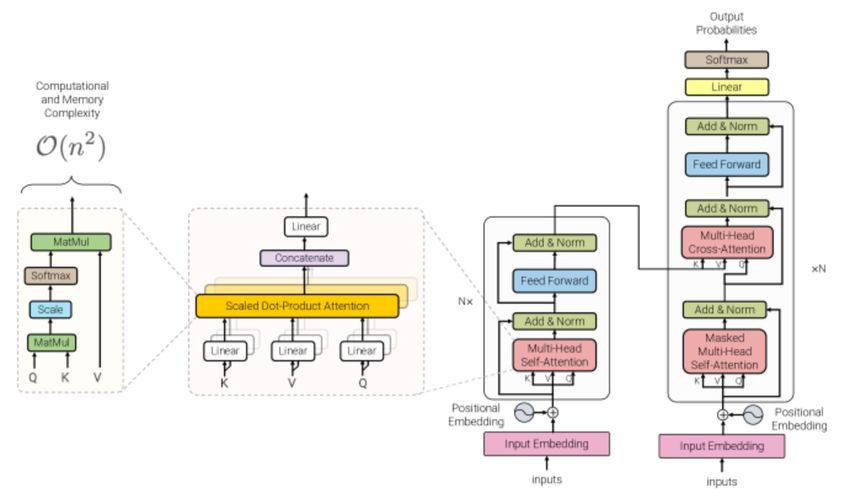
Introduced by [39], this involves taking the attention score of a sequence with respect
to the sequence itself to determine which parts of the sequence are the most important.
The attention score is calculated using the input sequence as the query, key and value
vector. In our model we have calculated attention score using scaled dot product
attention. The attention score is calculated n_head times, where n_head is the number
of heads of self-attention. The n_head self-attention scores are then concatenated
together to form the Multi-Head Attention (MHA) score.

 Figure 4.1.2.1 Transformer architecture [41]

The MHA layer forms a part of the Transformer Encoder layer, where the output of
the MHA layer is fed into a normalisation layer, followed by a feed forward layer (FF).
At each layer normalisation layer, the output of the MHA or FF is added to the original
input from the previous layer (a sub layer connection). The encoder layer is stacked
‘N’ times, with the output of the final layer passed into a linear ‘decoder’ layer to
provide the final prediction.

• Positional embedding/embedding/sequence representation

In transformer architecture there is no inherent notion of sequence input so we need to
represent the position of each input relative to the rest of the input space. We have
attempted to use 3 methods to do this, with varying results as detailed in section 7 –
Results.

 1. Time Embedding

Introduced by [40] and based on the implementation by [42], in this technique we use
the equation below to calculate the position of our sequence of features relative to other
input sequences within the same batch. We calculate the time embedding for the
features at each timestep according to the below formula. Each timestep has a linear
embedding and a sine embedding and the result is concatenated with the original
feature vector.

 ∗ + = 0
 Embedding at ti = I [40]
 ( ∗ + ) 1 ≤ ≤ 

 OHLC + 13 features (dim: n_features per timestep) Time embedding(dim : 2 per timestep)

 Figure 4.1.2.2 Time Embedding

 2. Positional Encoding

Positional encoding is a technique used in NLP tasks where the position of each
token input is given a position embedding relative to its position in the sequence. For
a timestep t and position i within the sequence, each input is given an embedding
based on whether it is on an odd or even index within the sequence.
 (#) sin( % . ) , = 2 
 ! = ( )# = ( ) = 4 [16]
 cos ( % . ), = 2 + 1

 1
 ℎ % = &%
 10000 '

 3. LSTM

LSTMs process data in a sequential manner so we have attempted to use a single
LSTM layer to capture the sequential aspect of our input data. The output of the
LSTM layer is fed into the stacked encoders in our experiment.

4.1.3 Auto Encoder + CNN + LSTM:

A hybrid model combining stacked autoencoder, CNN and LSTM for forecasting
foreign exchange rates is proposed.
Stacked Autoencoder
Manual extraction of features is more difficult in the context of lack of experience in
technical forex trading. Autoencoder is a neural network consisting of an input layer,
an output layer and a hidden layer, which can automatically extract features from the
input data and was first introduced in 1985 [35]. Stacked autoencoder is a simple
autoencoder to increase the depth of its hidden layer to obtain better feature extraction
ability and training effect. The key idea of autoencoder is to compress the
dimensionality of the input data to the number of neurons specified in the encoding
layer and then expand to the original dimensionality for reconstruction, forcing the
model to extract key features from the data by comparing the output with the initial
data.

Figure 4.1.3.1 Architecture of SAE

In this project we use a 2-layer stacked autoencoder architecture, and since the stacked
autoencoder is symmetric about the hidden layer, 4-layer full architecture is formed,
including two encoders and two decoders (see figure 4.1.3.1). The output of the
previous hidden layer is used as the input of the next hidden layer. We have one
hundred and 8 units in the input encoder layer, and the coding dimension is 27. L1
regularization, is added to reduce the risk of overfitting.

CNN-LSTM model

This model can be divided into four parts, input layer, CNN layers, LSTM layer and
dense layers (output layer). The input layer is used to receive the relevant data, then
the data will be input into the CNN layers. The CNN layers are consisted of 1D-
convolution layer, max pooling layer. The 1D- convolution layer can extract the
feature from each sample since all of the features for a point-in-time is in a row.
After the convolution is done, the dimension of the data is too large for the
convolution kernel, thus, the max pooling layer is carried out to reduce the
dimensions of the neural network to avoid overfitting. Then the output of CNN layer
will be the input of the LSTM layer. Due to the mechanism of LSTM model which
are including forget gate, input gate, output gate and memory cell, it can selectively
forget the memory of the input data, thus, the LSTM layer is used for predicting the
exact value. The architecture of the CNN-LSTM model is show in figure 4.1.3.2.

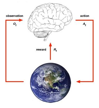
Figure 4.1.3.2: Architecture of CNN-LSTM model
Also, various hyperparameter are involved in the architecture development of this
model, through fine tuning these hyperparameters and measuring the accuracy of the
validation accuracy, the model has the best performance under the current
architecture. The hyperparameters are shown in the Table 4.1.3.3.
 Table n: Hyperparameter of CNN-LSTM model
 Hyperparameters Value
 Convolution Layer Filters 108
 Convolution Layer Kernel size 2
 Convolution Layer Activation Function sigmoid
 Convolution Layer kernel initializer uniform
 Pooling Layer Pool size 1
 Pooling Layer Padding valid
 Number of LSTM Layer Hidden Units 108
 LSTM Layer Activation Function tanh
 Time step 9
 Optimizer adam
 Loss Function mse
 Epochs 50
 Batch size 60
 Table 4.1.3.3

4.1.4 Reinforcement Learning:

Our aim of using the RL model (reinforcement learning model) is to generate trading
strategy. There are many different algorithms for the reinforcement learning, such as
Sarsa, deep Q network, and policy gradient. The main differences between all these
RL models lie in the methods each model uses to update the policy. However, they
all need the same elements including agent, environment, state (observation), action
and reward. The agent learns from the environment, executes actions based on the
state of the environment (or observations), and try to perform an action which can

lead to a higher reward. The algorithm selection and parameter tuning can influence
the performance of the model.

 Figure 4.1.4.1. Simple schematic diagram of the reinforcement learning process
1. Action: trading strategy. It is the output of the agent and the input of the
environment. In this project, actions are 0 (sell) and 1 (Buy)

2. State (observation) is the output of the environment and the input of agent. In this
project, state is the historical data of the foreign exchange market.

3. Reward is the output of the environment and the input of the agent. In this project,
reward is the cumulative profit we can obtain from the foreign exchange market.

4. Environment is a place where the agent is trained. In this project, environment is
the foreign exchange market.

5. Agent is the brain in Figure 4.1.4.1. It output the action based on the input
information and will keep learning until the reward meets the certain requirements.

6. Policy is a mapping of the probability distribution from state to action.

In this foreign exchange marker project, our goal is to identify the right time to buy
or sell and make profits from the market. This seems to be suitable for using a value-
based algorithm. However, for a value-based model, calculating the Q value and
selecting actions based on the Q value will become too complicated for a large
amount of data, such as time series data. Secondly, according to the conclusions
drawn by Thomas G. Fischer [1], the actor-only approach has a better performance
than other methods. Policy is a probabilistic strategy with stronger randomness and
flexibility. As a result, we chose policy gradient as our main algorithm for this
project.

The objective function is shown below.

 ( ) = # ( ) # ( , ) ( , ) (6)
 
Where % ( ) is the time spend on the statement s, & is the policy under parameter
vector , r is the reward.

The policy gradient function is:

 ! ( ! ) = # " ( ) # ! ! ( , ) " ( , ) (7)
 # $

where ' is the expectation of the reward.

We can observe that since we need to integrate two variables at this time, namely action
 and statement . It not only needs to consider the state probability distribution, but
also the action probability distribution, which increases the computational complexity.

The evaluation of the RL model will be carried out from the following points. The first
one is reward curve. By observing whether the curve rises or falls, we will be able to
determine whether the model performs good or not. Second, we can decide whether
our model can bring us profit by observing the revenue of the RL model on the test
dataset.

4.2 Data Collection

Data can be collected from various website/sources such as Yahoo financials or Oanda
using API. In our case, the OHLC data have been collected and provided to us by our
tutor in CSV format.

4.3 Data Analysis

We use Talib to calculate a group of technical indicators that can be derived from the
OHLC data. Most of our models are mainly focusing on a few different types of
technical indicators: moving average which uses long terms and short-term EMA and
SMA, MACD, DMI and momentum indicators which uses RSI and stochastic

oscillation. Please see below visual for various technical indicators vs price movement:

 Fig 4.3.1

5. RESULTS
5.1 Clustering + Attention model:

We have implemented and evaluated the clustering + attention model based on
different key parameters including various input sequence length, various future
prediction window sizes, different k values in K-means clustering and different cluster
threshold in Birch clustering as well as model’s performance across different currency
pairs. We split dataset from Jan2005 to Jan2020 at a ratio of 80/20 for training and
evaluating models’ performance (MSE, RMSE and MAE in below tables). We have
also heldout one year of data (from Feb2020 to Feb2021) for backtesting purpose only
to simulate feeding unseen data into our trained model then to calculate potential profit
and loss based on our trading strategy.

In regard to backtesting, we have developed a trading strategy to evaluate how much
profit & loss our model can make based on unseen data (Feb20 – Feb21). First, a long
position is opened when predicted high price of next hour is higher than current close
price (current close price is treated as our entry price in this case). Second, leverage
(200x) only applies when the predicted high price is at least 2xMAE higher than
current close price. When it comes to exit strategy, there are two scenarios that we exit

our long position. First, if the real price reaches the predicted price within next 60 mins
then the long position will be closed: profit/loss = predicted high price – entry price -
spread. Second, if the real price does not reach our predicted price within next 60 mins,
we exit the long position at the end of the 60 mins: profit/loss = closing price in 60
mins – entry price - spread. Here, we use 0.8 bps as the spread between AUD/USD
and this spread also include any commissions/brokage fees. Please see below tables
for all the experiment results:

 Cluster method K-means K-means K-means K-means K-means
 Currency Pair AUD/USD AUD/USD AUD/USD AUD/USD AUD/USD
 Next 60 Next 60
 Forecast Period mins Next 60 mins Next 60 mins mins Next 60 mins
 last 90 last 105 last 120 last 135
 Input Sequence mins mins mins mins last 150 mins
 # of cluster 8 8 8 8 8
 MSE 5.749E-07 5.471E-07 6.018E-07 4.093E-07 7.381E-07
 RMSE 0.0007582 0.000739662 0.000775758 0.0006398 0.000859127
 MAE 0.0005069 0.000503785 0.00054785 0.000489 0.00055423
 Backtest Data
 Period 1 year 1 year 1 year 1 year 1 year
 Max Leverage
 Ratio 200 200 200 200 200
 Spread 0.00008 0.00008 0.00008 0.00008 0.00008
 Backtest P&L
 with $10k initial
 capital $17,659 $11,296 $23,699 $13,926 $4,059
 Lowest Capital
 level based on
 trades $8,703 $9,890 $9,888 $7,525 $7,473
 Lowest Capital
 level based on
 Minimum price
 hit $6,472 $6,050 $6,048 $5,425 $2,277
 Worst Trade ($820) ($5,940) ($5,940) ($5,940) ($5,940)
 Best Trade $6,237 $3,553 $4,641 $3,934 $3,017
 Table 5.1.1 model’s performance on next 60 min with various input seq length

 Cluster method K-means K-means
 K-means K-means
 Currency Pair AUD/USD AUD/USD
 AUD/USD AUD/USD
 Next 90 Next 90
 Next 90 Next 90
 Forecast Period mins mins mins mins
 last 90 last 120
 last 150 last 180
 Input Sequence mins mins mins mins
 # of cluster 8 8 8 8
 MSE 1.086E-06 8.496E-07 1.159E-06 1.0547E-06
 RMSE 0.00104211 0.000921737 0.0010763 0.001026986

MAE 0.0006615 0.0006079 0.0006716 0.0006645
Backtest Data Period 1 year 1 year 1 year 1 year
Max Leverage Ratio 200 200 200 200
Spread 0.00008 0.00008 0.00008 0.00008
Backtest P&L with $10k initial capital $16,140 $31,718 $20,419 $12,331
Lowest Capital level based on valid trades $9,947 $8,372 $9,946 $6,437
Lowest Capital level based on Minimum
price hit $9,321 $6,103 $6,106 $3,857
Worst Trade ($60) ($3,180) ($3,180) ($3,180)
Best Trade $4,340 $4,012 $4,484 $4,041
 Table 5.1.2 model’s performance on next 90 min with various input sequence length

Cluster method K-means K-means K-means K-means
Currency Pair AUD/USD AUD/USD AUD/USD AUD/USD
 Next 120 Next 120 Next 120
Forecast Period mins mins mins Next 120 mins
 last 120 last 150 last 180
Input Sequence mins mins mins last 210 mins
# of cluster 8 8 8 8
MSE 1.2936E-06 1.0893E-06 1.2903E-06 0.000001221
RMSE 0.001137365 0.001043695 0.001135914 0.001104989
MAE 0.000734432 0.000676212 0.000742177 0.000750904
Backtest Data Period 1 year 1 year 1 year 1 year
Max Leverage Ratio 200 200 200 200
Spread 0.00008 0.00008 0.00008 0.00008
Backtest P&L with $10k initial
capital $22,628 $32,264 $25,786 $29,757
Lowest Capital level based on
valid trades $9,448 $1,598 $9,795 $9,898
Lowest Capital level based on
Minimum price hit $8,787 ($484) $9,377 $6,082
Worst Trade ($3,780) ($5,120) ($820) ($1,600)
Best Trade $4,635 $4,894 $6,237 $6,336
 Table 5.1.3 model’s performance on next 120 min with various input sequence length

Cluster method K-means K-means K-means K-means K-means K-means
 AUD/US AUD/US AUD/US
Currency Pair AUD/USD AUD/USD AUD/USD D D D
 Next
 next 30 Next 45 next 60 next 75 Next 90 105
Forecast Period min mins min min mins mins
 last 90 last 90 last 90 last 90 last 90 last 90
Input Sequence mins mins mins mins mins mins
# of cluster 8 8 8 8 8 8
 7.98E- 0.00000 1.2771E
MSE 3.648E-07 4.292E-07 5.749E-07 07 1086 -06
 0.000603 0.000655 0.000758 0.00089 0.00104 0.00113
RMSE 987 134 222 33 2113 009
 0.000393 0.000448 0.000506 0.00057 0.00066 0.00071
MAE 61 492 943 7 15 7
Backtest Data
Period 1 year 1 year 1 year 1 year 1 year 1 year
Max Leverage Ratio 200 200 200 200 200 200
Spread 0.00008 0.00008 0.00008 0.00008 0.00008 0.00008
Backtest P&L with
$10k initial capital $3,750 $9,951 $17,659 $13,955 $16,140 $16,953
Lowest Capital
level based on valid
trades $9,396 $9,881 $8,703 $8,910 $9,947 $7,296
Lowest Capital
level based on
Minimum price hit $8,396 $7,617 $6,472 $6,816 $9,321 $5,210
Worst Trade ($7,220) ($4,340) ($820) ($2,100) ($60) ($3,240)
Best Trade $2,258 $2,545 $6,237 $3,090 $4,340 $4,439
 Table 5.1.4 model’s performance on various prediction window size using last 90 mins data

Cluster method K-means K-means K-means K-means
Currency Pair AUD/USD CAD/USD NZD/USD CHF/USD
 Next 60 Next 60 Next 60
Forecast Period mins mins mins Next 60 mins
 last 135 last 135 last 135
Input Sequence mins mins mins last 135 mins
# of cluster 8 8 8 8
MSE 4.093E-07 1.0859E-06 6.48E-07 0.000001084
RMSE 0.00063977 0.001042065 0.000805 0.001041153
MAE 0.00048903 0.00066738 0.000587 0.0007442
Backtest Data Period 1 year 1 year 1 year 1 year
Max Leverage Ratio 200 200 200 200
Spread 0.00008 0.0002 0.0002 0.00017
Backtest P&L with $10k
initial capital $13,926 $14,371 $2,050 $19,308
Lowest Capital level based on
valid trades $7,525 $9,755 $5,721 $1,072

Lowest Capital level based on
Minimum price hit $5,425 $7,648 $607 ($1,188)
Worst Trade ($5,940) ($5,700) ($6,060) ($8,340)
Best Trade $3,934 $5,742 $3,386 $5,113
 Table 5.1.5 model’s performance on different currency pairs

Cluster method K-means K-means K-means K-means
Currency Pair JPY/USD EUR/USD GBP/USD JPY/GBP
 Next 60 Next 60
Forecast Period mins Next 60 mins mins Next 60 mins
 last 135 last 135
Input Sequence mins last 135 mins mins last 135 mins
# of cluster 8 8 8 8
 3.5705E-
MSE 1.5953 1.1539E-06 06 10.81685
 0.001889
RMSE 1.26305186 0.0010742 577 3.288897992
Test MAE +1 epoch vs above 1.0716 0.00075566 0.00101 2.7524
Backtest Data Period 1 year 1 year 1 year 1 year
Max Leverage Ratio 200 200 200 200
Spread 0.01 0.00008 0.00013 0.02
Backtest P&L with $10k ($1,211,75
initial capital 6) $3,635 $13,748 ($924,372)
Lowest Capital level based ($1,484,84
on valid trades 6) $9,999 $9,141 ($2,331,331)
Lowest Capital level based ($1,594,84
on Minimum price hit 6) $9,037 $2,254 ($4,188,441)
Worst Trade ($672,000) ($32) ($11,060) ($2,912,000)
Best Trade $912,000 $3,645 $6,775 $744,000
 Table 5.1.6 model’s performance on different currency pairs

Cluster method Birch Birch Birch Birch Birch Birch
Currency Pair AUD/USD AUD/USD AUD/USD AUD/USD AUD/USD
 AUD/USD
Cluster Threshold 0.01 0.05 0.1 0.2 0.3 0.5
 Next 60 Next 60 Next 60 Next 60 Next 60
 Next 60
Forecast Period mins mins mins mins mins mins
 last 135 last 135 last 135 last 135 last 135
 last 135
Input Sequence mins mins mins mins mins mins
 8 but
 8 but 8 but system
 system system only
 only only generate
# of cluster 8 8 8 generate 5 generate 5 3
MSE 6.46E-07 6.917E-07 5.123E-07 5.205E-07 8.336E-07 9.414E-07
RMSE 0.000803 0.00083169 0.00071575 0.00072146 0.00091302 0.0009703
MAE 0.000522 0.00054037 0.0005196 0.0004985 0.0005616 0.0005952
Backtest Data
Period 1 year 1 year 1 year 1 year 1 year 1 year

Max Leverage
Ratio 200 200 200 200 200 200
Spread 0.00008 0.00008 0.00008 0.00008 0.00008 0.00008
Backtest P&L with
$10k initial capital $15,228 $17,034 $12,028 $5,401 $7,198 $9,522
Lowest Capital
level based on
valid trades $9,995 $9,992 $5,296 $7,281 $2,753 ($75,912)
Lowest Capital
level based on
Minimum price
hit $8,506 $8,396 ($1,584) $5,185 ($1,387) ($89,091)
Worst Trade ($120) ($5,940) ($5,940) ($2,180) ($5,940) ($29,840)
Best Trade $3,175 $3,436 $3,234 $2,881 $3,123 $15,918
 Table 5.1.7 model’s performance using Birch cluster (k=8) with different Cluster Threshold value

Cluster method Birch Birch Birch Birch
Currency Pair AUD/USD AUD/USD AUD/USD AUD/USD
Cluster Threshold 0.01 0.05 0.1 0.2
Forecast Period Next 60 mins Next 60 mins Next 60 mins Next 60 mins
Input Sequence last 135 mins last 135 mins last 135 mins last 135 mins
 10 but system
# of cluster 10 10 10 reduces to 9
MSE 1.24E-06 8.128E-07 8.571E-07 6.195E-07
RMSE 0.001112 0.00090155 0.0009258 0.000787083
MAE 0.000564 0.0005645 0.0005769 0.0005149
Backtest Data Period 1 year 1 year 1 year 1 year
Max Leverage Ratio 200 200 200 200
Spread 0.00008 0.00008 0.00008 0.00008
Backtest P&L with
$10k initial capital $20,824 $23,267 $7,765 $5,115
Lowest Capital level
based on valid trades $9,910 $9,986 $9,827 $9,600
Lowest Capital level
based on Minimum
price hit $8,351 $8,435 $6,835 $5,791
Worst Trade ($800) ($61) ($5,940) ($5,940)
Best Trade $6,628 $6,353 $3,761 $2,767
 Table 5.1.8 model’s performance using Birch cluster (k=10) with different Cluster Threshold value

Cluster method K-means K-means K-means K-means K-means K-means
Currency Pair AUD/USD AUD/USD AUD/USD AUD/USD AUD/USD AUD/USD
 Next 60 Next 60 Next 60 Next 60 Next 60 Next 60
Forecast Period mins mins mins mins mins mins
 last 135 last 135 last 135 last 135 last 135 last 135
Input Sequence mins mins mins mins mins mins
# of cluster 1 2 3 4 5 6
MSE 1.02E-06 8.54E-07 1.11E-06 6.84E-07 6.84E-07 5.18E-07
RMSE 0.001008 0.000924 0.001052 0.000827 0.000827 0.00072
MAE 0.00066 0.000607 0.000585 0.000559 0.00054 0.000513
Backtest Data
Period 1 year 1 year 1 year 1 year 1 year 1 year
Max Leverage Ratio 200 200 200 200 200 200
Spread 0.00008 0.00008 0.00008 0.00008 0.00008 0.00008
Backtest P&L with
$10k initial capital ($8,082) $29,094 $15,143 $12,842 $1,295 $20,661
Lowest Capital
level based on valid
trades ($127,510) ($49,644) ($52,152) $5,721 $2,097 $9,995
Lowest Capital
level based on
Minimum price hit ($140,690) ($62,824) ($65,332) $1,581 ($847) $8,374
Worst Trade ($29,840) ($29,840) ($29,840) ($5,940) ($5,940) ($5,940)
Best Trade $14,227 $15,141 $15,009 $3,280 $3,088 $3,400
 Table 5.1.9 model’s performance using k-means cluster with different k value

Cluster method K-means K-means K-means K-means K-means K-means
Currency Pair AUD/USD AUD/USD AUD/USD AUD/USD AUD/USD AUD/USD
 Next 60 Next 60 Next 60 Next 60 Next 60 Next 60
Forecast Period mins mins mins mins mins mins
 last 135 last 135 last 135 last 135 last 135 last 135
Input Sequence mins mins mins mins mins mins
# of cluster 7 8 9 10 11 12
MSE 7.5E-07 4.093E-07 4.26E-07 4.63E-07 4.78E-07 4.76E-07
RMSE 0.000866 0.0006397 0.000653 0.000681 0.000691 0.00069
MAE 0.000542 0.000489 0.000474 0.000509 0.000495 0.000475
Backtest Data Period 1 year 1 year 1 year 1 year 1 year 1 year
Max Leverage Ratio 200 200 200 200 200 200
Spread 0.00008 0.00008 0.00008 0.00008 0.00008 0.00008
Backtest P&L with $10k
initial capital $5,983 $13,926 $7,317 $7,153 $6,034 $2,331
Lowest Capital level
based on valid trades $9,998 $7,525 $4,474 $1,911 $9,878 $9,895
Lowest Capital level
based on Minimum price $8,371 $5,425 $127 ($2,809) $6,038 $7,935
Worst Trade ($5,940) ($5,940) ($5,440) ($5,440) ($62) ($2,160)
Best Trade $2,723 $3,937 $3,253 $3,454 $3,149 $2,434
 Table 5.1.10 model’s performance using k-means cluster with different K value

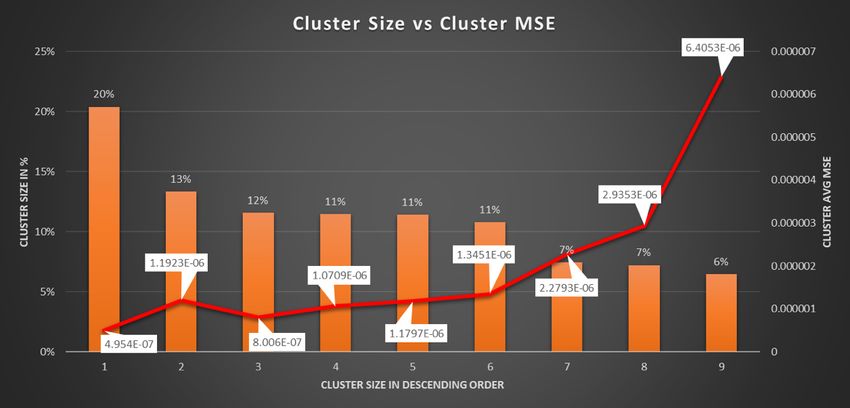
Cluster method K-means K-means K-means K-means K-means K-means
Currency Pair AUD/USD AUD/USD AUD/USD AUD/USD AUD/USD AUD/USD
 Next 60 Next 60 Next 60 Next 60 Next 60 Next 60
Forecast Period mins mins mins mins mins mins
 last 135 last 135 last 135 last 135 last 135 last 135
Input Sequence mins mins mins mins mins mins
# of cluster 13 14 15 16 17 18
MSE 6.78E-07 4.91E-07 4.52E-07 8.6E-07 4E-07 4.25E-07
RMSE 0.000824 0.000701 0.000673 0.000927 0.000632 0.000652
MAE 0.000638 0.000542 0.000483 0.000791 0.000468 0.000472
Backtest Data Period 1 year 1 year 1 year 1 year 1 year 1 year
Max Leverage Ratio 200 200 200 200 200 200
Spread 0.00008 0.00008 0.00008 0.00008 0.00008 0.00008
Backtest P&L with
$10k initial capital $5,354 $7,297 $2,310 $2,235 $2,301 $310
Lowest Capital level
based on valid trades $9,905 $9,998 $9,910 $4,486 $1,885 $4,487
Lowest Capital level
based on Minimum
price hit $6,065 $6,486 $7,881 $139 ($2,835) ($140)
Worst Trade ($2,160) ($2,160) ($2,160) ($5,440) ($5,440) ($5,440)
Best Trade $3,348 $2,984 $2,340 $4,712 $3,268 $3,082
 Table 5.1.11 model’s performance using k-means cluster with different K value

Cluster method K-means K-means K-means K-means
Currency Pair AUD/USD AUD/USD AUD/USD AUD/USD
 Next 60 Next 60 Next 60 Next 60
Forecast Period mins mins mins mins
 last 135 last 135 last 135 last 135
Input Sequence mins mins mins mins
Percentage 20% 13% 12% 11%
Accumulative 20% 34% 45% 57%
Cluster Size 3297 2156 1866 1851
Cluster # 1st 2nd 3rd 4th
MSE 4.954E-07 1.19E-06 8.01E-07 1.07E-06
RMSE 0.000703847 0.001092 0.000895 0.001035
MAE 0.0005075 0.000609 0.000687 0.000743
 Table 5.1.12 performance by cluster with k-mean (k=9)

Cluster method K-means K-means K-means K-means K-means
Currency Pair AUD/USD AUD/USD AUD/USD AUD/USD AUD/USD
 Next 60 Next 60 Next 60 Next 60 Next 60
Forecast Period mins mins mins mins mins
 last 135 last 135 last 135 last 135 last 135
Input Sequence mins mins mins mins mins
Percentage 11% 11% 7% 7% 6%
Accumulative 68% 79% 86% 94% 100%
Cluster Size 1844 1741 1201 1165 1042

Cluster # 5th 6th 7th 8th 9th
 MSE 1.18E-06 1.35E-06 2.28E-06 2.94E-06 6.41E-06
 RMSE 0.001086 0.00116 0.00151 0.001713 0.002531
 MAE 0.000723 0.000755 0.000788 0.00122 0.002236
 Table 5.1.13 performance by cluster with k-mean (k=9)

Final result on test data:

In this scenario, we split the 15 mins AUD/USD dataset to training (02Jan2005-
02Apr2019) and testing (03Apr2019 – 28Feb2021) right at the beginning before any
feature generation or shuffling. We also keep 24 hours gap between training and testing
data just to ensure there is zero information leakage from testing to training (since all
features are calculated based on information that are no longer than past 4 hours). Then
we generate features for training and testing separately and all models including
clustering was trained based on training data only. Please see below model’s
performance based on test data:

 Cluster method Kmeans
 Currency Pair AUD/USD
 Forecast Period next 60 mins
 Input Feature last 135 mins
 # of cluster 8
 Test MSE 0.00000063
 Test RMSE 0.000793725
 Test MAE +1 epoch vs above 0.00061
 1 year and 11
 Backtest Data Period months
 Max Leverage Ratio 200
 Spread 0.00008
 Backtest P&L with $10k initial capital $24,709
 Lowest Capital level based on valid trades $9,990
 Lowest Capital level based on Minimum price
 hit $6,475
 Worst Trade ($5,939)
 Best Trade $3,988
 Table 5.1.14

5.2 Transformer Multi Head Attention

The data is split up as 60% training, 20% validation and 20% test. All results are based
on predictions on test data. All outputs are after training for 20 epochs and with
learning rate of 0.1 using SGD optimizer and a batch size of 6 is used during training.

Method Best MSE Best RMSE Best MAE
 Time embedding + Transformer Encoder 0.000416866 0.020417293 0.00901897
 Positional encoding + Transformer Encoder 1.679615 1.29599 1.24654
 Time embedding+positional encoding + 1.796017 1.34015 1.29238
 Transformer encoder
 LSTM + Transformer Encoder 2.290292 1.5133 1.47123
 LSTM + Time Embedding +Transformer 0.0079 0.089 0.066
 Encoder
 Transformer Encoder only 0.002223 0.047155 0.04386

The following results are from using time embedding and transformer encoder.

 Number of encoder
 Test MSE Test RMSE Test MAE
 layers
 1 0.00107 0.03273 0.01824
 2 0.00077 0.02786 0.014399
 3 0.00055 0.02365 0.007808
 4 0.00081 0.02847 0.009055
 5 0.00062 0.02494 0.019219
 6 0.00058 0.02412 0.00875
 Table 5.2.2: 4 heads = 4, d_k, d_v = 10, ff_dim = 32

 Parameters Test MSE Test RMSE Test MAE
 n_head = 1, d_k, d_v = 10 0.02236 0.14953 0.08529
 n_head = 2, d_k, d_v = 10 0.000806 0.02839 0.01244
 n_head = 4, d_k, d_v = 10 0.00055 0.02365 0.007808
 n_head = 8, d_k, d_v = 10 0.000416866 0.020417293 0.00901897
 n_head = 4 d_k, d_v = 4 0.000437085 0.02090659 0.00732209
 n_head = 4 d_k, d_v = 19 0.00047899 0.021885 0.0118105
 n_head = 8 d_k, d_v = 25 0.0009038 0.0300633 0.0162498
 n_head = 4, d_k = 25, d_v
 = 35
 0.00055879 0.023638 0.008724
 Table 5.2.3 : 3 encoders, ff_dim = 32

 Parameters Test MSE Test RMSE Test MAE
 Conv1d FFN d_ff = 128 0.000557 0.023613 0.00785
 Conv1d FFN d_ff = 64 0.00045212 0.02126329 0.008011466
 Conv1d FFN d_ff = 32 0.00055 0.02365 0.007808
 Conv1d FFN d_ff = 16 0.00644 0.08025 0.04356
 Conv1d FFN d_ff = 8 0.0004727 0.021743 0.01574
 Linear FFN d_ff = 128 2.29029 1.51337 1.47123
 Linear FFN d_ff = 8 2.319159 1.522878 1.48101
 Table 5.2.4 : 3 encoders, 4 heads, d_k, d_v =10

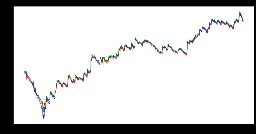
Currency
 MSE RMSE MAE
 Pair
 AUD/USD 0.000416866 0.020417293 0.00901897
 EUR/USD 0.09946 0.31537 0.2159
 NZD/USD 4.03248 x 10-5 0.00635 0.004527
 CAD/USD 0.17537 0.41878 0.28885
 GBP/USD 0.13925 0.37316 0.31377
 CHF/USD 0.12856 0.35855 0.29731
 JPY/USD 0.5648103 0.75153 0.726237
 EUR/AUD 0.21321 0.461748 0.38735
 Table 5.2.5 : 3 encoders, 4 heads, d_k, d_v = 10, ff_dim = 32

5.3 Auto Encoder + CNN + LSTM:

To avoid data leakage and accurately simulate the real prediction environment. We use
the last year of data as the test set for back testing. The first 80% of the remaining data
is used as the training set and the last 20% as the validation set. The hybrid model
combined with CNN and LSTM was used as the benchmark model, and the prediction
performance of the model was evaluated by comparing the MAE, MSE and RMSE
results of the model on the validation set. Figure 5.3.1 shows the predicted data and
the corresponding actual data for two models using AUD/USD 15min data to predict
the maximum price for the next hour. Figure 5.3.2 shows the results of running our
model on the main 8 currency pairs.

Figure 5.3.1 Actual(blue) and predicted from SAE+CNN+LSTM (red), CNN+LSTM (green) model for
AUD/USD.

Figure 5.3.2 Comparison of the performance results for two different models on the main 8 currency
pairs

5.4 Reinforcement learning

First, we tried different parameters, different input data fragments with different data
lengths using AUD_USD_M15 dataset and test the performance of the RL model on
the test dataset. The results are given in Figure5.4.1 and the parameter configuration
are given in Table 5.4.3. We can observe that for the same dataset, the reward curve
for both train dataset and test dataset are very different. Although different
parameters have been tried, the model failed to perform as we expected.

Figure5.4.1. Results under different parameters (left-Model A, right-Model B)

The best model result we achieved is shown in Figure7.4.2. The input data length is
800. We also applied this model on the forecast data generated by the regression
model to output a corresponding trading strategy. Because the data is predictive data
and the order of the data is disrupted, we cannot test the model on the real data.

 Figure5.4.2. Best result on AUD_USD_M15 dataset (Model C)

Form the figure above, we can conclude that the RL model has a better performance
on the predicted data than the test dataset. So, we infer that the RL model may be
more suitable for predicting the data that is stationary. Another inference is that the
prediction data generated by the regression model contains certain features, which
helps the RL model to make better decisions and obtain higher rewards. Details will
be discussed in the next section.

 Data length Layer size Episodes Profits
 Model A 0.0006 800 128 8000 -0.05%
 Model B 0.0001 1600 256 8000 -0.03%
 Model C 0.0002 800 128 5000 1.18%
 Table 5.4.3 The corresponding parameters for 3 models

(Note: is the learning rate)
In addition to performing experiments using different parameters on the same
dataset, we tried to perform the experiments using the same parameters on different
datasets. This experiment helped us to find which currency pair will bring us more
profits than the others. To ensure the uniformity, all our models will use the same
parameters configuration, which is given in the following table.

 Input Data length Layer size Episodes Test data length
 0.0002 1600 128 12000 800

 Table 5.4.4. Unified parameters configuration for different currency pairs

After the retraining all 7 models, we came to the following result.

 Dataset Profits Dataset Profits
 AUD_USD_M15 4.92% GBP_JPY_M15 10.15%
 USD_CAD_M15 6.95% GBP_USD_M15 1.14%
 NZD_USD_M15 4.58% USD_JPY_M15 0.68%
 EUR_USD_M15 2.26% USD_CHF_M15 4.075%

 Table 5.4.5. Profits generated by the RL model for different currency pairs

 Figure 5.4.6. Environmental rendering for GBP_JPY_M15 (red-sell, green-buy)

Among the eight most traded currencies, we found that our model made the most
profit on the GBP_JPY pair, reaching a profit of 10%, but not so good on the other
currency pairs.

6. DISCUSSION
6.1 Clustering + Attention:

Based on the experiment results above, it shows that to predict high price for next 60
mins using last 135 mins sequence length yields the lowest MSE. For next 90 mins
high price prediction, using last 120 mins as input sequence length yields the lowest
MSE. And for next 120 mins high price prediction, using last 150 mins as input
sequence length yields the lowest MSE. Please see below graph for price prediction
performance for different window sizes.

 Next 60 mins prediction
 0.0000008

 0.0000006
 MSE

 0.0000004

 0.0000002

 0
 last 90 mins last 105 mins last 120 mins last 135 mins last 150 mins
 Input Sequence

 Next 90 mins prediction
 0.0000015

 0.000001
 MSE

 0.0000005

 0
 last 90 mins last 120 mins last 150 mins last 180 mins
 Input Sequence

 Next 120 mins prediction
 0.0000014
 0.0000013
 0.0000012
 MSE

 0.0000011
 0.000001
 0.0000009
 last 120 mins last 150 mins last 180 mins last 210 mins
 Input Sequqnce

 Figure 6.1.1

When input sequence length is fixed at past 90 mins, it works the best with predicting
the next 30 mins high price (MSE ~3.65e-07) vs worst performance when predicting
the next 105 mins (MSE ~1.28e-06). The reason behind is probably due to smaller
pricing fluctuation or movement for shorter period (i.e. price movements within 30
mins on average is smaller than ones in 60 mins). And the smaller price movement
will lead to a smaller prediction MSE (see figure 6.1.2). Furthermore, a

 Performance with 90 mins input sequence vs prediction
 window size
 0.0000014
 0.0000012
 0.000001
 0.0000008
 MSE

 0.0000006
 0.0000004
 0.0000002
 0
 next 30 min Next 45 mins next 60 min next 75 min Next 90 mins Next 105 mins
 Future Prediction Window

 Figure 6.1.2

smaller prediction window size means it is less likely for an instance to be impacted
by events such as release of CPI data. For example, if to predict the next 2 days of
foreign exchange price movement, it is more likely that we can have some news that
could impact the price than if to make prediction for the next 30 mins. Thirdly, with a
smaller prediction window size we can have more data i.e. we can have 24 times more
data point when predicting next hour than next day’s high price. And for most of
machine learning models, performance is positively correlated with number of training
data. In regard to backtesting P&L, results showing that P&L for smaller window size
(i.e. next 30 mins) is limited at ~$3750 (even though it has got smaller MSE) vs ones
with large window size (i.e. next 60 mins) ~ $17659 (see below figure 6.1.3). This is
because larger price movement usually leads to higher profit margin but with higher
risk as well (“lowest capital level” is worse for next 105 mins prediction vs next 30
mins prediction see figure 6.1.4).

Backtest P&L vs different predict window size
 $20,000
 $18,000
 $16,000
 $14,000
 Backtest P&L $12,000
 $10,000
 $8,000
 $6,000
 $4,000
 $2,000
 $0
 next 30 min Next 45 mins next 60 min next 75 min Next 90 mins Next 105
 mins

 Figure 6.1.3

 Capital Level vs Predition Win Size
 $12,000
 Lowest Capital Level

 $10,000
 $8,000
 $6,000
 $4,000
 $2,000
 $0
 next 30 min Next 45 next 60 min next 75 min Next 90 Next 105
 mins mins mins
 Prediction Win Size

 Figure 6.1.4

The model’s performances across various currency pairs are different which
AUD/USD performs the best and this is probably because AUD/USD is the currency
pair we use to train and test our model during every phase of the experiment including
feature selection and parameter tuning. It means all the features are selected based on
AUD/USD and it might not be the best one for some other currency pairs. And this is
especially true for Japanese Yan which is a 2 bps currency pair and results showing
our model works poorly against Japanese Yan.

We have also implemented another clustering algorithm – birch. Overall, its optimal
performance is very similar to k-means in terms of MSE, RMSE and MAE. One of the
key parameters in Birch is cluster threshold. It decides the maximum distance between
datapoint for them to be grouped together. In another word, a higher cluster threshold

means cluster is more generalised and data are much easier to be grouped together. As
per our experiment results, model’s performance in terms of both MSE and backtest
P&L got much worse when cluster threshold is larger than 0.2.

 Validation MSE vs Cluster Threshold (Birch)
 0.000001

 0.0000005

 0
 0.01 0.05 0.1 0.2 0.3

 Figure 6.1.5

To find the optimal K value in kmeans clustering, a series of values (from 1 to 18) has
been tested. As below graph (fig 6.1.6) shows that test MSE tends to reduce along with
higher K. With a small K, the model is not making enough number of sub-groups
meaning it tends to allocate data with different pattern into the same clusters. On the
other hand, when K is assigned with a large number (i.e. k=16) the performance is
stagnated with too many unnecessary clusters. One of the reasons is because we now
have less data in every cluster meaning the model is more likely to overfit due to a
smaller training data size. Furthermore, for backtesting result between different K
value, even though model’s MSE (8.54E-07) at K=2 is much worse than K=8 (4.093E-
07) theK=2 backtest P&L ($29k) is much higher than K=9 ($14k). This is because the
model with k=2 makes more risky trades and it is reflected in capital status: for k=2
its 10k initial capital hit negative during the period meaning its position could have be
liquidated by broker. On the other side, the lowest capital level for K=8 is $5.5k based
on $10k initial capital shows that a higher K with smaller MSE might not generate the
largest profit but will make safer trades for less risk.