HOMEOWNER BORROWING AND HOUSING COLLATERAL: NEW EVIDENCE FROM EXPIRING PRICE CONTROLS
←
→
Page content transcription
If your browser does not render page correctly, please read the page content below
HOMEOWNER BORROWING AND HOUSING COLLATERAL:
    NEW EVIDENCE FROM EXPIRING PRICE CONTROLS∗

                                      Anthony A. DeFusco†
                                  Kellogg School of Management
                                    Northwestern University

                                                July 1, 2015
                                                    Abstract
       I empirically analyze how changes to the collateral value of real estate assets affect home-
       owner borrowing behavior. While previous research has documented a positive relationship
       between house prices and home-equity based borrowing, a key empirical challenge has been
       to disentangle the role of collateral constraints from that of wealth effects in generating this
       relationship. To isolate the role of collateral constraints, I exploit the expiration of resale
       price controls on owner-occupied housing units created through an inclusionary zoning reg-
       ulation in Montgomery County, Maryland. Because the duration and stringency of the price
       controls are set by formula and known in advance, their expiration has no effect on expected
       lifetime wealth but directly shocks collateralized borrowing capacity. Using data on all trans-
       actions and loans secured against every property in the county from 1997–2012, I estimate
       that the marginal propensity to borrow out of increases in housing collateral induced by ex-
       piring price controls is between $0.04 and $0.13. The magnitude of this effect is correlated
       with a homeowner’s initial leverage and indicates that a significant fraction of the additional
       borrowing arising from house price increases is due to relaxing collateral constraints. Addi-
       tional analysis of residential investment and ex-post loan performance further suggests that
       borrowers used at least some portion of the extracted funds to finance current consumption
       and investment expenditures. These results highlight the importance of collateral constraints
       for homeowner borrowing and suggest a potentially important role for house price growth
       in driving aggregate consumption.

   ∗
      I am deeply indebted to my advisors Gilles Duranton, Fernando Ferreira, Joe Gyourko, Nick Roussanov, and
Todd Sinai for their guidance and support. Tom Davidoff, Jessie Handburry, Dan Sacks, Maisy Wong, and Yi-
wei Zhang as well as seminar participants at Berkeley (Haas), Harvard (HBS), Indiana University (Kelley), London
Business School, London School of Economics, Northwestern (Kellogg), Notre Dame (Mendoza), University of
Chicago (Booth), UCLA (Anderson), UPenn (Wharton), WUSTL (Olin), the CFPB, the Federal Reserve Board,
and the WFA Summer Real Estate Symposium provided helpful comments and discussion. I am also thankful to
Stephanie Killian and Maureen Harzinsky in the Montgomgery County Department of Housing and Community
Affairs and to Diana Canales at SunTrust Bank for providing useful details on inclusionary zoning and the financing
of price-controlled housing units in Montgomery County. All errors are my own.
    †
      Kellogg School of Management, Northwestern University, 4215 Donald P. Jacobs Center, 2001 Sheridan Road,
Evanston, IL 60628; E-mail: anthony.defusco@kellog.northwestern.edu.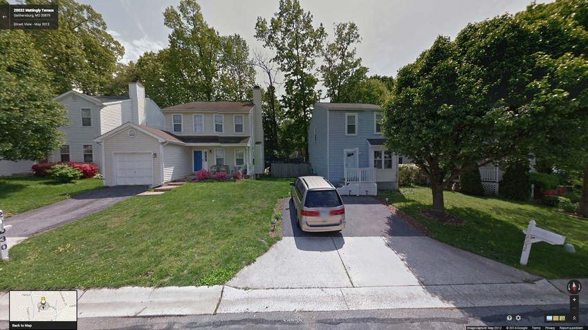
I.    INTRODUCTION
By some accounts, over half of the mortgage debt accumulated in the U.S. during the run-up
to the Great Recession can be directly attributed to the effect of rapidly rising house prices on
the demand for home equity debt among existing homeowners (Mian and Sufi, 2011). This can
be seen clearly in Figure I, which plots aggregate trends in house prices and home equity debt
relative to income over the period 1990–2014.1 The pattern is stark. At the same time that house
prices were rising, existing homeowners were taking out an increasingly large amount of debt
against their homes—debt that they quickly began to off-load as prices collapsed.
     Why do homeowners respond to rising house prices in this way? In standard models, an
increase in house prices may lead homeowners to take on additional debt due to both a direct
effect on household wealth—rising prices make homeowners feel richer—and an indirect effect on
collateralized borrowing capacity—rising prices relax previously binding borrowing constraints
tied to the value of the home. The goal of this paper is to isolate the empirical relevance of the
latter channel by studying how the borrowing behavior of individual homeowners responds to
changes in the collateral value of their homes.
     Isolating the independent effect of collateral constraints from that of wealth effects is impor-
tant from the perspective of macroeconomic policy because the two mechanisms have markedly
different implications for the way in which house price changes spill over into aggregate eco-
nomic activity. By propagating the effects of small shocks throughout the economy, increases
in homeowner borrowing driven by the relaxation of binding collateral constraints have the po-
tential to generate large swings in aggregate consumption (Bernanke and Gertler, 1989; Kiyotaki
and Moore, 1997; Iacoviello, 2005). In contrast, increases in homeowner borrowing driven by
wealth effects are likely to have a limited impact since they will typically be offset by decreases
among renters, for whom higher house prices represent a negative wealth shock (Sinai and Soule-
les, 2005; Campbell and Cocco, 2007; Buiter, 2008). Therefore, knowing whether and to what
extent collateral constraints drive individual homeowner borrowing behavior is central to our
understanding of how house price changes affect the real economy and to the debate over how
monetary policy should respond to such changes in prices.
     Existing empirical research, however, has struggled to provide direct estimates of the effect of
collateral values on homeowner borrowing. Two key challenges have hindered progress. First,
it is difficult to identify situations in which changes to the collateral value of a house occur inde-
pendently from changes to the owner’s housing wealth. As a result, most analyses have focused
   1
     Greenspan and Kennedy (2005, 2008) present similar time-series evidence using a broader measure of home
equity withdrawal that includes the proceeds from cash-out refinances and home sales. The measure used in this
figure includes only equity extraction occurring through home mortgages secured by junior liens and home equity
lines of credit.

                                                      1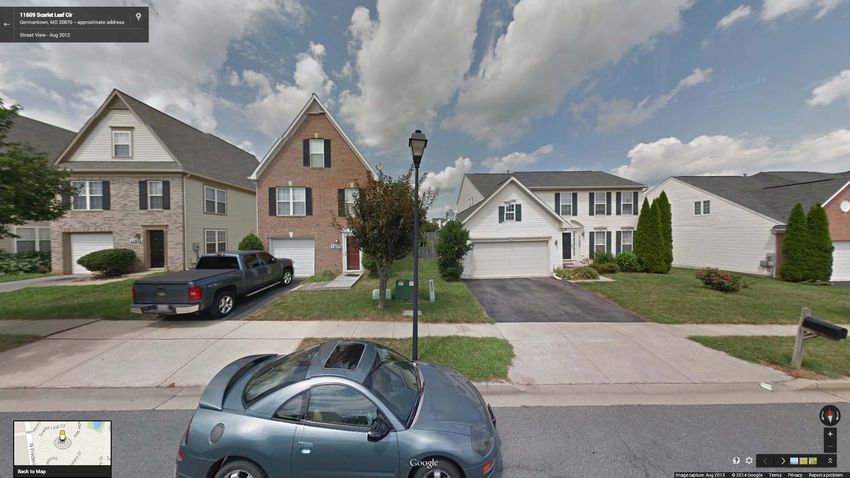
primarily on the overall effect of house prices on borrowing while attempting to infer the role
of collateral constraints through the use of indirect proxies—proxies that in many cases conflate
credit demand with credit supply (Gross and Souleles, 2002; Agarwal, Liu, and Souleles, 2007).2
Second, as in most empirical analysis, omitted variables and simultaneity biases loom large. Ag-
gregate shocks to joint determinants of house prices and homeowner borrowing, such as interest
rates and expected future income, make it exceedingly difficult to draw causal inferences from
naturally occurring changes in house prices, even when one is only interested in the overall rela-
tionship between prices and borrowing.3
    In this paper, I make use of an alternative approach to contribute new empirical estimates
of the causal effect of housing collateral on home equity-based borrowing. To isolate the effect
of collateral values from generalized wealth effects, I exploit a unique feature of local land use
policy in Montgomery County, Maryland that drives a wedge between the value of a house as
collateral and its value as a component of homeowner wealth. Since 1974, housing developers
in Montgomery County have been subject to an inclusionary zoning regulation known as the
Moderately Priced Dwelling Unit (MPDU) program. This policy requires developers to set aside
at least 12.5 percent of all housing units in new developments to be made available at controlled
prices to moderate-income households.4 These housing units are subject to deed restrictions that
cap their resale prices for a period of time ranging between 5 to 30 years. During this period,
owners are not permitted to refinance or take on home equity debt for an amount that exceeds
the controlled resale price. Once the price controls expire, however, owners are able to pledge the
full market value of the home as collateral. Since the duration and stringency of the price controls
are set by formula and known in advance at the time of purchase, their expiration has no effect
on the owner’s total expected lifetime wealth. However, expiring price controls directly affect
   2
      Recent papers using this approach to study various determinants of equity extraction include Hurst and Stafford
(2004); Yamashita (2007); Disney and Gathergood (2011); Mian and Sufi (2011, 2014); Cooper (2013) and Bhutta and
Keys (2014). There are also a host of studies using this approach to study consumption responses to house price
changes, many of which are reviewed in Bostic, Gabriel, and Painter (2009). Three important exceptions are Leth-
Petersen (2010), Abdallah and Lastrapes (2012), and Agarwal and Qian (2014), who study explicit policy-induced
changes in collateral constraints similar to the one studied in this paper. However, these studies rely on national- and
state-level policy variation, which makes it difficult to separately identify aggregate trends from household-specific
changes to collateral constraints.
    3
      A frequently proposed solution to this problem is to instrument for local house prices using Saiz’s (2010) esti-
mates of cross-city variation in physical constraints to building (Mian and Sufi, 2011, 2014; Aladangady, 2013; Mian,
Rao, and Sufi, 2013). However, as cautioned by Saiz (2010) and further emphasized by Davidoff (2011, 2014), phys-
ical supply constraints are highly correlated with a host of other demand factors that might be expected to directly
affect both house prices and homeowner borrowing. Moreover, as Davidoff (2014) demonstrates, physical building
constraints were not correlated with changes in the size of the housing stock during the 2000s, suggesting that the
correlation between house prices and building constraints was not necessarily operating through the constraints
themselves during that period.
    4
      For a four-person household, the maximum income limit is set at 70 percent of the median family income for
the Washington, D.C. metropolitan area. In 2014, that limit was $75,000, which is roughly 17 percent higher than
the national median family income that year.

                                                           2
the collateral value of the home through the relaxation of the borrowing restrictions. Leveraging
this fact, I show within the context of a stylized model of home equity-based borrowing that
differential changes in the propensity for MPDU homeowners to extract equity from their homes
at the time the restriction is lifted contain explicit information regarding the effect of collateral
values on homeowner borrowing. I then use that information to provide new estimates of both
the extensive margin effect of relaxing collateral constraints on home equity extraction and the
marginal propensity to borrow against a $1 increase in collateral value.
    To conduct my analysis, I assemble a unique dataset containing the precise geographic location
and detailed structural characteristics of every housing unit in Montgomery County as well as
the full history of transactions and loans secured against each property during the period 1997–
2012. I combine this information with administrative records from the Montgomery County
Department of Housing and Community Affairs, which identify the restricted housing units and
the dates for which the applicable price controls were in effect. This dataset allows me to identify
the effect of expiring price controls by comparing how the borrowing behavior and prices paid by
owners of controlled housing units changes following the expiration of the price control relative
to that of owners of nearby and observationally identical never-controlled units. It also allows me
to track the borrowing behavior of a given homeowner over time, permitting a within-ownership
spell comparison of equity extraction before and after the expiration of the price control. The
added degrees of freedom afforded by the fact that controlled units are dispersed relatively evenly
throughout the county and expire at different points during the sample period further allow me
to control flexibly for aggregate trends affecting borrowing behavior and for unobservable but
fixed differences across localities within the county.
    I find compelling evidence that increases in collateral values lead homeowners to extract eq-
uity from their homes. In housing developments containing controlled units, transaction prices
for the controlled units increase by roughly 40–65 percent relative to observationally identical
non-controlled units in the same development following the expiration of the price controls. In
response to these price gains, owners of controlled units are roughly four percentage points more
likely to extract equity from their homes in a given year after the expiration of the price con-
trol relative to owners of non-controlled units. This effect is large, representing an almost 100
percent increase over the pre-expiration mean probability of equity extraction among owners of
controlled units. Both the price effect and the increase in equity extraction among owners of
controlled units are immediately present in the year the price control expires and almost per-
fectly offset the gap that exists between owners of controlled and non-controlled units during
the imposition of the price control.
    Using information on the size of individual loans, I convert these figures into an estimate
of the marginal propensity to borrow against an increase in housing collateral. On average, I

                                                 3
find that a $1 increase in collateral values leads homeowners to extract between $0.04–$0.13 in
additional home equity debt. To put this into context, estimates from the literature of the over-
all effect of house prices on homeowner borrowing, which combine both collateral and wealth
effects, range between $0.06–$0.25.5 Thus, my estimates imply that collateral constraints can ex-
plain a sizable fraction of the effect of house price increases on homeowner borrowing, even in
the absence of any changes in perceived wealth.
     To provide additional evidence that collateral constraints are the dominant force leading own-
ers of price-controlled units to extract equity from their homes following the expiration of the
price control, I also investigate heterogeneity in the response across individuals. In particular, I
show that homeowners with high initial leverage (as measured by their loan-to-value (LTV) ratio
at the time of purchase) are far more likely to respond to expiring price controls by extracting
equity than homeowners with low initial leverage. I find no statistically or economically signif-
icant effects for homeowners in the bottom portion of the initial leverage distribution (LTV ≤
0.7), whereas the effects for the most highly levered households (LTV > 0.95) are both statisti-
cally significant and roughly twice as large as the overall average effect. These results suggest that
the increase in collateral values induced by the expiring price controls only affects borrowing
behavior among the subset of homeowners for whom collateral constraints were likely to have
bound prior to expiration.
     My empirical strategy identifies the effect of collateral values on equity extraction under the
assumption that borrowing behavior would have evolved similarly for owners of both controlled
and uncontrolled units in the absence of the expiring price control. To probe the validity of this
assumption, I conduct a range of different robustness checks. Most importantly, I provide direct
graphical evidence showing that the trends in outcomes for controlled and uncontrolled units
move together in the period prior to expiration and only begin to diverge once the price controls
expire. To more formally assess the validity of the parallel trends assumption, I also conduct a
series of placebo tests in which I randomly assign price control expiration dates to the controlled
units and re-estimate the main specifications. The results of this exercise suggest that the effects
I find are unlikely to have been generated by spurious correlation alone. The estimated effects
are also robust to the inclusion of both ownership spell fixed-effects and subdivision-specific time
trends, implying that any time-varying omitted factors driving the results must be present at
both the level of the individual homeowner and the particular housing subdivision in which her
home is located. Finally, to further address potential concerns regarding the comparability of
controlled and never-controlled units, I also replicate the main analysis using a semi-parametric
propensity score matching estimator.
   5
   See Haurin and Rosenthal (2006); Disney and Gathergood (2011); Mian and Sufi (2011, 2014), and Bhutta and
Keys (2014).

                                                     4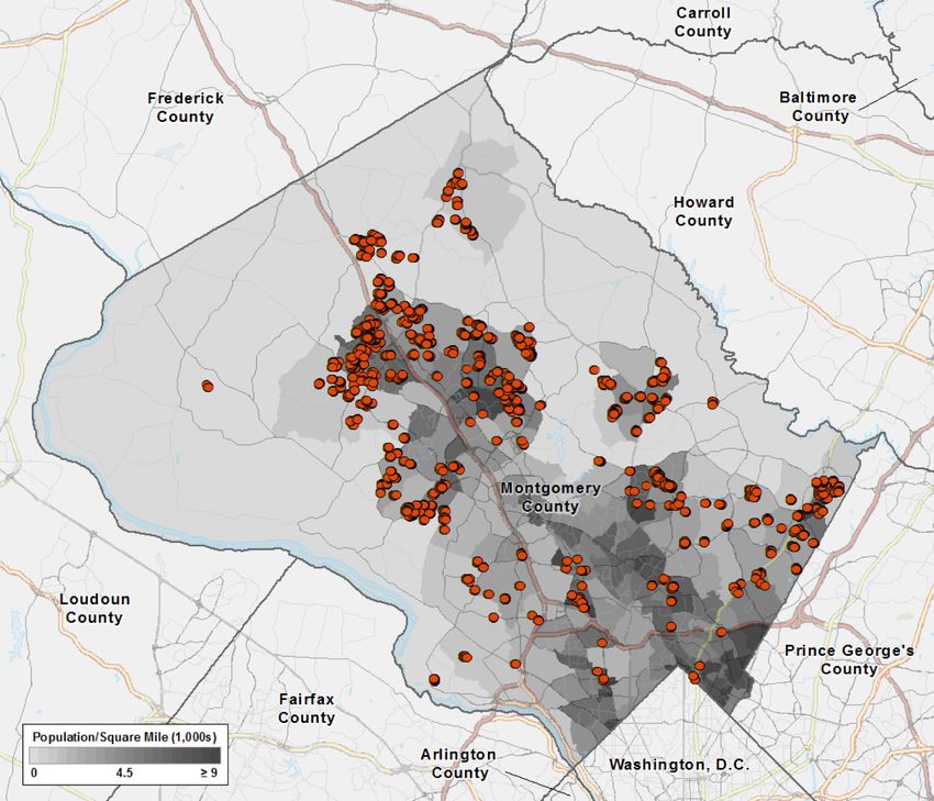
While my results provide clear evidence that homeowners respond to increases in housing
collateral by borrowing against their homes, the real effects of such borrowing depend on how
the money is used. In particular, if homeowners simply reinvest the proceeds into more-liquid
assets or use the funds to pay off other outstanding debt, then home equity-based borrowing
induced by rising collateral values should not be expected to affect current consumption or in-
vestment expenditures. Although limitations of the data prevent me from being able to provide
a full account of the uses of extracted funds, I provide two pieces of evidence suggesting that at
least some fraction of the borrowed money was used to fund current expenditures. First, us-
ing administrative data on building and home improvement permits issued by the Montgomery
County Department of Permitting Services, I find that the annual likelihood of applying for a
home improvement permit increases differentially by roughly 0.6–1 percentage points among
owners of price-controlled units following the expiration of the price control. This effect rep-
resents an increase of approximately 60–100 percent over the pre-expiration mean and suggests
that borrowers likely used some portion of the extracted equity to fund residential investment
expenditures.6 Second, the deeds data used to conduct the main analysis also contains informa-
tion on home foreclosures. Using this information, I show that the three-year foreclosure rate
associated with equity extractions secured against MPDU properties increases by roughly 1.5–2
percentage points relative to equity extractions secured against non-MPDU properties following
the expiration of the price control. This result is consistent with previous findings regarding the
increased risks associated with house price-induced equity extraction and suggests that borrowers
are unlikely to be reinvesting all of the proceeds into more-liquid assets, as their risk of foreclo-
sure would presumably remain unchanged if that were the case (Mian and Sufi, 2011; Bhutta and
Keys, 2014; Laufer, 2014).
    My findings build on a large empirical literature studying various relationships between house
prices and household consumption, savings, and borrowing behavior (recent examples include
Case, Quigley, and Shiller, 2005, 2013; Campbell and Cocco, 2007; Cooper, 2013; Gan, 2010;
Leth-Petersen, 2010; Carroll, Otsuka, and Slacalek, 2011; Disney and Gathergood, 2011; Mian
and Sufi, 2011, 2014; Abdallah and Lastrapes, 2012; Carroll and Zhou, 2012; Calormiris, Longhofer,
and Miles, 2013; Mian, Rao, and Sufi, 2013; Agarwal and Qian, 2014 and Bhutta and Keys, 2014).7
   6
      An alternative interpretation of this result is that the expiration of the price control increases the owner’s incen-
tives to invest in the home, as was documented by Autor, Palmer, and Pathak (2014) in the context of rent control,
and may therefore explain both the increase in permitting activity and the increase in equity extraction even in the
absence of any collateral effects. This is unlikely to be the case in my context because the formula used to determine
the controlled price is adjusted upward dollar-for-dollar to reflect documented home improvements. As a result,
the price control generates little disincentive for investment during the control period. Moreover, for owners who
plan to stay in the home beyond the end of the control period, the expected return from home improvements is
determined solely based on the market price. For these owners, the exact timing of the expiration therefore has no
effect on investment incentives.
    7
      Bostic, Gabriel, and Painter (2009) provide a useful review of the earlier literature in this area. A related literature

                                                              5
Many studies in this literature have attempted to infer the role that collateral constraints play in
generating these relationships between house prices and homeowner behavior through the use
of indirect proxies for constraints. For example, a common approach has been to explore how
households with different credit histories and incomes or at different points in the life cycle re-
spond to similar changes in house prices.8 While the results from these analyses are generally
suggestive of an important role for collateral constraints, the indirect nature of the proxy mea-
sures employed has left open the possibility that such estimates may be confounding differences
in constraints with differences in preferences. I contribute to this literature by providing the first
direct estimates of the collateral effect that leverage time-varying and household-specific changes
in access to housing collateral.
    This paper also relates to a much broader literature studying the role of collateral in the
macroeconomy. An important theoretical literature in macroeconomics emphasizes the role
that collateral constraints can play in amplifying business cycle fluctuations through the effect
of changes in asset prices on the borrowing capacity of both firms and households (see, for ex-
ample, Bernanke and Gertler, 1989; Kiyotaki and Moore, 1997; Iacoviello, 2005). Given that real
estate is such a large source of collateral for many households and businesses, a particular point
of focus in the empirical literature studying the microeconomic foundations underlying this “fi-
nancial accelerator” mechanism has been to examine how households and businesses respond to
changes in the collateral value of their real estate assets.9 This paper contributes new empirical
has also studied non-house price determinants of the demand for home equity debt, including income shocks (Hurst
and Stafford, 2004) and various other sources of macroeconomic uncertainty (Chen, Michaux, and Roussanov, 2013).
There is also an extensive literature studying the financial incentive to refinance an existing mortgage from an option
theoretic point of view (see, for example, Agarwal, Driscoll, and Laibson, 2013; Keys, Pope, and Pope, 2014, and
references therein.)
    8
      This approach is motivated by similar strategies that have been used to study the role of liquidity constraints in
the vast empirical literature estimating consumption and borrowing responses to various forms of income receipt
(see, for example, Zeldes, 1989; Jappelli, 1990; Shapiro and Slemrod, 1995; Jappelli, Pischke, and Souleles, 1998;
Parker, 1999; Souleles, 1999; Browning and Collado, 2001; Johnson, Parker, and Souleles, 2006; Agarwal, Liu, and
Souleles, 2007; Stephens, 2008; Aaronson, Agarwal, and French, 2012; Parker et al., 2013; Baker, 2014; Zhang, 2014
and many others as reviewed by Browning and Lusardi, 1996; Browning and Crossley, 2001; Jappelli and Pistaferri,
2010, and Zinman, 2014).
    9
      For example, several recent papers have provided empirical evidence on the firm side by documenting a siz-
able effect of real estate prices on corporate investment, capital structure, and credit terms (Benmelech, Garmaise,
and Moskowitz, 2005; Gan, 2007; Chaney, Sraer, and Thesmar, 2012; Cvijanovic̀, 2014), although Deng, Gyourko,
and Wu (2013) find no evidence of a real estate collateral channel on firm investment in China. A related set of
empirical papers has studied the relationship between house prices and entrepreneurship to test whether access to
collateralized debt through home mortgages is an important determinate of small business formation and employ-
ment (Hurst and Lusardi, 2004; Schmalz, Sraer, and Thesmar, 2013; Adelino, Schoar, and Severino, 2014; Jensen,
Leth-Petersen, and Nanda, 2014). Similarly, on the household side, Caplin, Freeman, and Tracy (1997) and Lustig
and Van Nieuwerburgh (2010) provide empirical evidence for a link between falling house prices, collateral con-
straints, and the consumption responses to regional income shocks in the U.S., while Almeida, Campello, and Liu
(2006) present cross-country evidence suggesting that both house prices and the demand for mortgage debt are more
sensitive to income shocks in countries with more generous collateral constraints.

                                                           6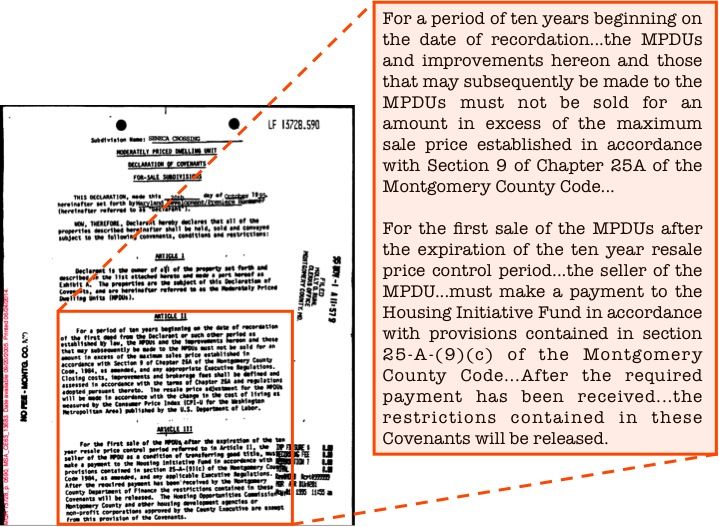
evidence on the household side by documenting a strong positive relationship between housing
collateral values and home equity-based borrowing.
The remainder of this paper is organized as follows: Section II provides institutional back-
ground on the Montgomery County Moderately Priced Dwelling Unit Program. Section III
discusses how MPDU price control expirations can be used to identify collateral effects in the
context of a stylized model of home equity extraction. The data sources and method used to
measure equity extraction are discussed in Section IV. Section V outlines the empirical research
design. Section VI presents the main estimates of the effect of expiring price controls on col-
lateral values and borrowing behavior. Evidence on the uses of extracted funds is presented in
Section VII, and Section VIII concludes.
II. THE MODERATELY PRICED DWELLING UNIT PROGRAM
Established in 1974, the Moderately Priced Dwelling Unit (MPDU) Program in Montgomery
County, Maryland is one of the oldest and most well-known inclusionary zoning policies in
the United States. Inclusionary zoning policies are local land use regulations that either require
or incentivize housing developers to set aside a fraction of their new developments to be sold
or rented to low- and moderate-income households at below-market prices. Historically, these
policies have been particularly popular in high-cost suburban areas; however, in response to rising
house prices and concerns over increasing spatial segregation on the basis of income, inclusionary
zoning policies have grown in popularity over the last 15 to 20 years and now exist in roughly
500 municipalities across 27 states, including several large urban centers such as New York, San
Francisco, Washington, D.C. and Chicago (Hickey, Sturtevant, and Thaden, 2014).
II.A. Developer Requirements
The MPDU program requires that any developer wishing to build a residential development
within the county containing more than 20 housing units must set aside a minimum of 12.5
percent of those units to be sold or rented to income-eligible households at controlled prices.10
Except in rare cases, the affordable units must be provided on-site and are subject to minimum
quality standards and planning guidelines that encourage the developer to scatter MPDUs among
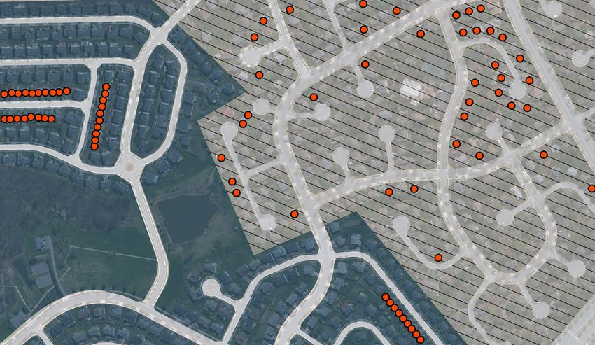
market-rate units in the same development. Figure II provides an example of the spatial distri-
bution of MPDUs in two representative subdivisions.11 In general, MPDU units tend to be dis-
tributed throughout the subdivision though design standards can lead to some clustering in large
10
If the developer agrees to provide more than the required 12.5 percent of affordable units, they are also granted
density bonuses that allow for the construction of more market-rate units than would otherwise be permitted under
the pre-existing zoning code. In practice, developers rarely take this option.
11
The data used to determine the location of the price-controlled units is described in detail in Section IV.
7subdivisions since MPDUs are typically smaller than many of the market-rate units and are there-
fore often placed alongside each other. While MPDUs are permitted to be smaller in terms of
interior square-footage and the construction standards provide some allowances for lower quality
interior finishes (e.g. counter-tops and bathroom fixtures), both the planning guidelines and the
private incentives of developers encourage the exterior design of MPDUs to reflect that of the
nearby market-rate units. This can be seen in Appendix Figure A.1.1, which provides pictures
of several example MPDUs and nearby market-rate units. Since its inception, the program has
resulted in the creation of roughly 14,000 housing units that were price-controlled at some point
in their history.12 As of the 2010 Census, these units represented roughly 3.7 percent of the total
stock of housing units in the county.13 Approximately 70 percent of the MPDUs were originally
offered for sale as owner-occupied units while the remainder were marketed as rentals. In this
paper, I restrict attention to the owner-occupied portion of the program.
II.B. Income Limits and Eligibility
Eligibility to purchase an MPDU is restricted to first-time homebuyers who qualify for a mort-
gage and whose annual gross household income falls within specified ranges published annually
by the Montgomery County Department of Housing and Community Affairs (DHCA). In the
frequent case in which more than one eligible buyer is interested in purchasing an MPDU, the
right to purchase is allocated by lottery.14 Minimum income limits are set at the same level for
all households and are meant to reflect the minimum income required to qualify for a typical
mortgage on an MPDU home. Maximum income limits are pegged to the median family income
for the Washington, D.C. metropolitan area as published by the U.S. Department of Housing
and Urban Development (HUD). For a four-person household, the maximum income limit is
set at 70 percent of the area median income for a household of the same size. That limit is then
scaled by an adjustment factor to determine the income limits for households of other sizes. The
income limits for 2014 are shown in Appendix Table A.1.1. In general, the income limits are
quite high, reflecting both the relative affluence of the D.C. metropolitan area and the fact that
the MPDU program is meant to specifically target moderate-income households. For example,
12
This figure is based on aggregate counts published by the Montgomery County Department of Housing and
Community Affairs (DHCA) at http://www.montgomerycountymd.gov/DHCA/housing/singlefamily/mpdu/
produced.html. The aggregate counts disagree slightly with the number of units for which I was able to obtain
microdata. This is likely due to changes in administrative record keeping that led some of the older units to drop
out of the DHCA database from which my data are derived.
13
This figure is less than the mandated 12.5 percent due primarily to the durability of the housing stock. Ac-
cording to the 2012 American Community Survey, the median housing unit in Montgomery County was built in
1977, implying that roughly half of the housing units in the county were built before the law went into effect. The
remaining gap is likely made up by housing units in smaller subdivisions to which the law does not apply.
14
The lottery gives preference to those living or working in the county and to those who have been on the waiting
list for multiple drawings.
8the maximum income limit of $75,000 for a four-person household is roughly 17 percent higher
than the 2014 national median income for a household of the same size. As will be discussed in
the data section below, this leads purchasers of MPDU homes to look relatively similar to the
typical homebuyer in the U.S., at least in terms of household income.
II.C. Price Controls and Borrowing Restrictions
The initial purchase price for an MPDU is set by the DHCA according to a schedule that is meant
to reflect construction costs associated with housing units of various types and sizes. Adjustments
are made on a square footage basis for unit sizes deviating from those specified in the schedule
and various “soft cost” adjustments are made in order to take into account developer financing
costs, overhead, and other miscellaneous fixed costs of construction.
Owners of MPDUs are permitted to resell their homes. However, if the sale occurs before
the end of the “control period” (a span of time ranging between 5 and 30 years depending on the
initial purchase date), then the resale price is capped at the original price plus an allowance for
inflation. Dollar-for-dollar adjustments are also made to account any documented major home
improvements. The resale restrictions are enforced through deed covenants that are tied to the
land and are released upon the first sale after the end of the control period (see Appendix Fig-
ure A.1.2 for an example deed covenant). Owners who sell before the end of the control period
must sell their home either directly to the DHCA or to another income-eligible household on
the waiting list. The first owner to sell the home after the end of the control period is permitted
to sell to any buyer at the market price but is required to split any capital gains over the controlled
price equally with the DHCA.
Appendix Table A.1.2 shows the history of rules governing the length of the control period.
Prior to 2002, the control period was set as a fixed period of time from the date of the initial
sale by the developer. Beginning in March 2002, the program was changed so that the control
period now resets if the unit is sold at any time prior to expiration. The length of the control
period was also extended from 10 years to 30 years in April 2005. These changes to the law
are reflected in Figure III, which plots the number of MPDU properties whose price controls
expired or will expire in each year since the inception of the program. The shaded grey area
marks the period of time during which I am able to observe transactions and loans.15 The 1980s
construction boom shows up as an increase in the number expiring price controls in the 1990s
while the boom associated with the most recent cycle will not show up until approximately 2035.
Of the price-controlled homes in my final analysis sample, roughly 92 percent had a 10 year initial
price control.
15
The transaction and loan data as well as the data used to determine the number of expiring price controls in
each year is discussed in detail in Section IV
9Importantly, the owner’s ability to borrow against the home is also restricted during the
control period. In particular, MPDU owners are prohibited from refinancing their mortgages
or taking on home equity debt for an amount that exceeds the controlled resale price. Thus,
while the appraised market value of the home may be substantially higher than the controlled
price, the owner is prohibited from pledging that equity as collateral until the expiration of the
price control. This requirement is enforced by both the DHCA and by lenders themselves, who
typically run title searches as part of the underwriting process, which would reveal any deed
restrictions placed on the property. After the price controls have expired, MPDU owners are no
longer restricted from borrowing more than the controlled price and, due to the shared profit
agreement, are typically able to pledge up to half of the difference between the controlled price
and the full market value as additional collateral.16 As discussed in detail in Section VI, I estimate
that the average discount for an MPDU home during the control period is between $66,000–
$106,000, implying an increase in collateralized borrowing capacity of roughly $33,000–$53,000.
Expiring price controls thus generally lead to a large increase in the collateral value of an MPDU
owner’s home, which, as the next section discusses, can be used to provide estimates of the effect
of changes in housing collateral on home equity-based borrowing.
III. CONCEPTUAL FRAMEWORK
To illustrate how expiring price controls can be used to identify the effect of housing collateral
on homeowner borrowing, this section presents a stylized model of a homeowner’s equity ex-
traction decision. I begin by considering a baseline model in which there are no price controls
in order to highlight the difficulties associated with disentangling collateral effects from wealth
effects using natural variation in house prices. I then show how the borrowing restrictions asso-
ciated with MPDU price controls can be used to address these difficulties. The basic structure
of this model draws heavily on Bhutta and Keys (2014), who use the same framework to study
the effect of interest rates on equity extraction. To keep the model simple and focus the discus-
sion on distinguishing collateral from wealth effects, I abstract from several issues that might be
present in a more fully-specified life-cycle model but would otherwise not permit an analytical
solution.17 Most importantly, I assume that house prices and income are known with certainty,
that households enter the world endowed with a house and a mortgage, and that they only live
for two periods during which they may use their home as a source of collateral and as a source of
wealth to fund consumption but from which they receive no direct utility.
16
This is because lenders are aware of the owner’s obligation to the county and are thus reluctant to extend credit
for an amount beyond what the owner would receive in the event of sale.
17
For examples of fully specified life-cycle models that incorporate the home equity extraction decision, see Hurst
and Stafford (2004) or Chen, Michaux, and Roussanov (2013).
10III.A. Baseline Case: No Price Controls
Consider a household that lives for two periods, t ∈ {0, 1}, and is endowed with a house of value
H and outstanding mortgage debt M0 in the first period. The household has log preferences
defined over non-housing consumption in each period, u t (c t ) = l o g (c t ), receives per-period in-
come, y t , and may extract equity by borrowing against the home in the first period, b0 , at the
going mortgage interest rate, r , and up to an exogenous collateral constraint λH − M0 , λ ∈ [0, 1].
The household chooses consumption in each period to maximize total lifetime utility
max U (c0 , c1 ) = l o g (c0 ) + βl o g (c1 ), (1)
c0 ,c1
subject to constraints which are given in the baseline case by
c0 = y0 + b0 (2)
c1 = y1 − (1 + r )(M0 + b0 ) + ωH (3)
0 ≤ b0 ≤ λH − M0 , (4)
where β ∈ [0, 1] is the discount factor and ω ∈ [0, 1] captures, in a reduced form way, the house-
hold’s desire to consume out of housing wealth.
Differences in the parameter ω across households can arise from various sources. For exam-
ple, in a life-cycle model with finitely lived households, ω will vary according to age. Younger
households who plan to continue living in the same house for a longer period of time likely have
lower values relative to older households who may choose to downsize in the near future (Camp-
bell and Cocco, 2007). Similarly, ω may vary within age group due to differences in bequest
motives, which lead households who wish to leave more to the next generation to consume less
of their housing wealth before death. Or, as in Sinai and Souleles (2005), ω may vary by expected
tenure length and by the correlation in house prices across markets to which a household is likely
to move in the future. Modeling the housing wealth effect in this way, while somewhat ad hoc,
greatly simplifies the discussion and is meant to capture these sources of heterogeneity without
needing to specify a particular mechanism through which the wealth effect arises. The impor-
tant point is that for some households who plan to consume part of their housing wealth before
death, increases in house prices will lead to a desire to smooth consumption across periods.
Substituting the per-period budget constraints (2) and (3) into the objective function (1) and
11solving for the optimal level of equity extraction yields the solution
y + ωH − (1 + r )(M0 + βy0 )
b∗ ≡ 1
b ∗ < λH − M0 (5a)
b0 =
∗ (1 + r )(1 + β)
λH − M0
b ∗ ≥ λH − M0 (5b)
where b ∗ denotes the optimal level of borrowing in the absence of the collateral constraint. This
expression highlights the empirical difficulties associated with using natural variation in house
prices to disentangle collateral effects from wealth effects. To see this, consider the effect of an
exogenous increase in house prices on equity extraction. For unconstrained borrowers, this effect
is given by the partial derivative of (5a) with respect to H and is a pure wealth effect, whereas for
constrained borrowers, it is equal to the partial derivative of (5b) and operates entirely through
the collateral constraint. The empirically observable change in borrowing is therefore given by:
ω
∂ b0∗ b ∗ < λH − M0 (6a)
= (1 + r )(1 + β)
∂H λ b ∗ ≥ λH − M0 , (6b)
where (6a) is the wealth effect for unconstrained borrowers and (6b) is the collateral effect for
constrained borrowers. Without prior knowledge of b ∗ , it is impossible to know which of these
two conditions applies for a given household and therefore impossible to know how much of the
observed average change in borrowing in response to a change in house prices is due to wealth
effects or collateral constraints.
The typical approach to solving this problem has been to infer the role of collateral constraints
by examining how the magnitude of the borrowing response varies across different populations
for whom one might expect either (6a) or (6b) to be the more relevant condition. For example,
we might expect that not only are younger households more likely to have values of ω close to
zero, but they are also more likely to have larger values of b ∗ as a result of steeply sloped life-cycle
wage profiles that generate a gap between current and future income (y1 > y0 ). Thus, if younger
homeowners are observed to increase borrowing more than older homeowners in response to
similar increases in house prices, this could be taken as evidence for the importance of collateral
constraints. However, as noted by Jappelli (1990), younger households might also be expected
to be less constrained than older households if the rate of time preference is low relative to the
real interest rate and consumption profiles are increasing in age. This ambiguity highlights the
difficulty of using indirect proxy measures such as age to infer the role of collateral constraints
and may explain why studies that do so have found mixed evidence (Campbell and Cocco, 2007;
12Mian and Sufi, 2011; Bhutta and Keys, 2014).18
Another common approach is to examine heterogeneity in responsiveness across borrowers
M
with different levels of prior debt utilization (M0 ) or loan-to-value ratios ( H0 ), which shift the
right-hand side of the inequality determining whether (6a) or (6b) applies. In this case, a finding
that borrowers with higher loan-to-value ratios or prior debt utilization rates are more responsive
to changes in prices is often taken as evidence in favor of collateral constraints (Disney and Gath-
ergood, 2011; Mian and Sufi, 2011; Mian, Rao, and Sufi, 2013).19 Similarly, several authors have
investigated heterogeneity based on differences in income, liquid assets, or credit scores, with
high-income, more-liquid, and high-credit score households expected to be less affected by col-
lateral constraints (Yamashita, 2007; Mian and Sufi, 2011, 2014; Cooper, 2013; Bhutta and Keys,
2014). While these proxies, and loan-to-value ratios in particular, are more direct measures of col-
lateral constraints than a homeowner’s age, such proxies are nonetheless limited by their reliance
on relatively strong a priori assumptions that are required in order to identify the set of poten-
tially constrained households—assumptions that in many cases conflate credit demand with credit
supply (Gross and Souleles, 2002; Agarwal, Liu, and Souleles, 2007). For instance, it is unclear
whether homeowners with higher initial LTVs or fewer liquid assets borrow more in response to
house price increases because they were unable to borrow prior to the change in prices (collateral
constraints) or simply because they have stronger consumption smoothing motives that led them
to carry more debt in the first place (wealth effects). More generally, as these examples illustrate,
indirect proxy measures are inherently limited in their ability to distinguish differences in col-
lateral constraints from other potential sources of heterogeneity, thus highlighting the need for
estimates that are based on a more direct approach.
III.B. Identifying Collateral Effects Using MPDU Expiration Dates
The borrowing restrictions associated with MPDU price controls drive a wedge between the
value of a home as collateral and its value as a component of homeowner wealth that allows for
a direct test of the role of collateral constraints. To see this, note that during the control period,
an MPDU owner is prohibited from borrowing against the full market value of the property and
therefore faces a more stringent collateral constraint so that equation (4) becomes
0 ≤ b0 ≤ λ(H − η) − M0 , (7)
18
Appealing to similar reasoning, Cooper (2013) finds larger consumption responses among households who ex-
perience higher realized future income growth and argues that this is evidence in favor of the role of collateral
constraints.
19
In related work, Hurst and Stafford (2004) also use loan-to-value ratios as a proxy for collateral constraints in
studying how equity extraction responds to changes in interest rates.
13where η ≥ 0 denotes the MPDU price discount. For an MPDU owner who plans to stay in the
home beyond the end of the control period, the eventual resale value of the home in the second
period, H , remains unchanged and the optimal level of borrowing can be found by replacing
equation (4) with equation (7) and resolving the borrower’s problem:20
y + ωH − (1 + r )(M0 + βy0 )
b∗ ≡ 1
b ∗ < λ(H − η) − M0 (8a)
b0∗ = (1 + r )(1 + β)
λ(H − η) − M0
b ∗ ≥ λ(H − η) − M0 . (8b)
In this framework, an expiring price control is equivalent to lowering the value of η to zero
in the first period while leaving the eventual resale price of the home in the second period, H ,
unchanged. To see how this affects borrowing, note that the effect of a decrease in η on b0∗ is
given by:
∂ b0∗ b ∗ < λ(H − η) − M0
¨
0 (9a)
− =
∂η λ b ∗ ≥ λ(H − η) − M0 . (9b)
This expression makes immediately clear that borrowing should only respond to an expiring
price control through the behavior of households who were collateral constrained prior to expi-
ration. Comparing (9a) with (6a), we can see that there is no longer any role for wealth effects.
Thus, any observed changes in borrowing behavior at the time the price control is lifted can
be entirely attributed to the effect of relaxing collateral constraints. This is the key insight un-
derlying the empirical analysis. In the following sections, I provide empirical estimates of the
magnitude of this response by studying how the borrowing behavior of MPDU owners changes
around the time the price control expires relative to that of owners of observationally identical
market-rate units in the same housing development for whom there is no corresponding change
in collateral values.
IV. DATA AND MEASUREMENT
To conduct the empirical analysis, I merge data at the property, transaction, and loan level us-
ing information from tax assessments, deeds records, and administrative data from the MPDU
program. This section provides a brief overview of the data sources, variable construction, and
sample selection procedures. Further details are available in Appendix A.2.
20
Here, H should be thought of as the owner’s expected proceeds from selling the home, net of the profit sharing
agreement with the county. While the price control affects the amount of profit sharing, the key point is that for
owners who plan to stay in the home beyond the end of the control period, that effect is fully anticipated so that the
actual timing of the price control expiration has no effect on the expected proceeds from selling the home.
14IV.A. Data Sources
Property-Level Data
The basic structure of my dataset is organized around the 2011 Montgomery County property
tax assessment file, which provides a single snapshot of all taxable properties in the county as of
2011. This file was purchased from DataQuick, a private vendor that collects and standardizes
publicly available tax assessment and deeds records from municipalities across the U.S. The tax
assessment file includes detailed information on the physical characteristics (e.g. square footage,
number of bathrooms, number of stories, year built), use type (e.g. residential, commercial,
single-family, condo), and street address for every property in the county. From this file, I drop
all non-residential and multi-family properties as well as any properties with missing characteris-
tics.21 This leaves a “universe” of 286,484 single-family residential properties from which I select
my analysis sample. Each of these properties is geocoded and assigned a subdivision ID based
on whether the geographic coordinates for the property fall within the boundaries of a partic-
ular subdivision, as delineated by the Maryland State Department of Assessments and Taxation
(SDAT).22
To identify MPDU homes, I match the property assessment file with a list of MPDUs scraped
from a publicly available online search portal hosted by the DHCA.23 This data provides me
with the street addresses for all MPDU properties in the DHCA administrative database as well
as the price control expiration dates for those properties. MPDU properties were matched to
the assessment file using a combination of exact physical location (geographic coordinates) and
street address as described in Appendix A.2.A. Of the roughly 8,300 MPDUs in the DHCA
database, I am able to match approximately 90 percent to a property in the assessment file.24
Figure IV maps the location of these properties as well as census tract-level population density
for Montgomery County in 2010. In general, MPDU properties are evenly distributed across the
21
The assessment data in Montgomery County is of unusually high quality. Only 3,702 out of 290,186 single-
family residential properties are dropped due to having missing characteristics. In 3,258 of these cases, it is the year
built that is missing while other characteristics, such as square footage and number of bathrooms, are coded as zero,
suggesting that many of these properties were vacant land at the time of assessment.
22
The subdivision boundary file was created using a parcel-level boundary file provided by the Montgomery
County Planning Department. In addition to the geographic boundaries, this file also contains the SDAT subdivi-
sion ID for each parcel. The subdivision boundaries were constructed by dissolving the individual parcel boundaries
into larger polygons based on whether they shared the same subdivision ID.
23
The search portal can be accessed at http://www6.montgomerycountymd.gov/apps/DHCA/pdm_online/
pdmfull.asp and was scraped by running a script that exhaustively searched through and returned all possible
MPDU addresses beginning with an alpha-numeric character.
24
The match rate is lower than 100 percent largely due to poor quality record keeping in the DHCA database for
some of the older MPDU properties. For example, when matching on street address, I require an exact match on
the street number. Some of the older MPDU properties are missing street numbers and are therefore not included
in the set of matches.
15non-rural regions of the county. One exception is the southern region of the county immediately
bordering Washington, D.C., where MPDUs are underrepresented. This region contains the
cities of Bethesda and Silver Spring and was developed much earlier than the rest of the county.25
As a result, much of the housing stock in that area was not subject to the MPDU regulations at
the time of development.26
Transaction and Loan-Level Data
To analyze how expiring price controls affect collateral values and homeowner borrowing, I
merge the property-level file with two additional datasets from DataQuick. Both datasets are
sourced from local deeds records and can be linked to properties in the assessment file using a
unique property ID. The first dataset contains information on all housing transactions occurring
in the county during the period 1997–2012. For each transaction, this dataset records the pur-
chase price, buyer, seller, and lender names, as well as loan amounts on up to three loans used to
finance the purchase. The second dataset contains information on all non-purchase loans secured
against a property during the same period. This dataset records the initial loan amount and bor-
rower and lender name for every refinance, junior lien, and home equity line of credit (HELOC)
secured against a property. Together, these two datasets provide me with a highly granular and
near complete picture of all mortgage borrowing and housing purchases occurring in the county
during this period. Each dataset is cleaned as described in Appendix A.2.B in order to ensure that
the transactions represent true ownership-changing arm’s length transactions and that the loan
information is accurate and consistent.
IV.B. Measuring Equity Extraction
Since the non-purchase loans dataset contains a combination of loan types but does not distin-
guish between them, several steps must be taken in order to construct an accurate measure of
equity extraction. In particular, it is important to distinguish between three different types of
non-purchase loans: (1) regular refinances, which replace an existing loan without extracting any
equity; (2) cash-out refinances, which replace an existing loan with a larger loan, thereby extract-
ing equity for the amount of the difference; and (3) new non-purchase originations, which directly
extract equity for the amount of the new loan. In order to make this distinction, I construct a
“debt history” for every property that records an estimate of the current amount of outstanding
debt secured against the property at any point in time on up to two potential loans. Debt histo-
25
This can be seen in Appendix Figure A.2.1, which replicates Figure IV replacing population density with prop-
erty age.
26
Another reason for the underrepresentation of MPDUs in this region is that a larger fraction of the housing stock
in the most densely populated areas (i.e. central cities) is composed of rental properties, which are not included in
the MPDU data that I use.
16ries are constructed by amortizing prior loan balances using the average interest rate at the time
the loan was originated.27 Given this history, when a new loan is observed, I am then able to
determine whether that loan represents a purchase loan, cash-out refinance, new non-purchase
origination, or regular refinance by comparing the size of the new loan to the estimated outstand-
ing balance on the relevant existing loan (see Appendix A.2.C for the details of this procedure).
When a new refinance or purchase loan is observed, the old loan is replaced and the new loan
serves as the basis for calculating remaining debt going forward.
Having categorized loans in this way, I then construct an annual panel that records for each
property whether the current owner extracted equity in a particular year and if so, how much eq-
uity was extracted. I define total equity extraction in a given year as the sum of non-purchase orig-
inations and cash withdrawn through cash-out refinances during that year. Similarly, an owner is
defined as having extracted equity in a given year if total equity extracted is greater than zero. For
properties built prior to 1997, the panel covers the full sample period from 1997–2012; for proper-
ties built afterwards, the construction year is used as the first year of observation. Each observa-
tion is also uniquely associated with a particular “ownership-spell” for that property. Ownership
spells are defined to include all years between ownership-changing transactions, where the first
ownership spell starts in either 1997 or the year that the property was built. In Appendix A.2.C,
I provide details validating the accuracy of this equity extraction measure against two measures
provided at the aggregate level based on data from Equifax credit reports and the Freddie Mac
Quarterly Cash-Out Refinance report. In both cases, my measure of equity extraction is shown
to be highly correlated with national aggregates.
IV.C. Sample Restrictions and Descriptive Statistics
Starting with the full sample of 286,484 properties, I impose several restrictions in order to ar-
rive at my primary analysis sample. I first drop any property that could not be matched to a
housing subdivision. This eliminates 31,603 properties located primarily in rural and outlying
areas of the county where SDAT does not assign subdivision IDs. I further drop all properties
located in subdivisions containing no MPDUs. This restriction eliminates 167,117 properties,
many of which were located in densely populated areas consisting mostly of rental housing or in
older subdivisions to which the regulation did not apply. Among subdivisions containing MP-
DUs, I further require that at least one MPDU expires during the DataQuick sample period.
This eliminates 35,236 properties located in either older subdivisions containing only MPDUs
27
All loans are amortized using the average offered interest rate on a 30-year fixed rate mortgage in the month that
the loan was originated. Monthly average offered interest rates are taken from the Freddie Mac Primary Mortgage
Market Survey (PMMS). Since the DataQuick data do not distinguish between HELOCs and closed end liens, all
loans are treated as fully amortizing with an initial principal balance equal to the origination amount, which for
HELOCs, represents the maximum draw-down amount. See Appendix A.2.C for the details of this procedure.
17You can also read