ARBITRAGE AND PARITY CONDITIONS - IRP, PPP, IFE, EH & RW
←
→
Page content transcription
If your browser does not render page correctly, please read the page content below
ARBITRAGE AND PARITY
              CONDITIONS
                      IRP, PPP, IFE, EH & RW

              Arbitrage in FX Markets
Arbitrage Definition
It is an activity that takes advantages of pricing mistakes in financial assets in
one or more markets. It involves no risk and no capital of your own.

• There are 3 types of arbitrage
       (1) Local (sets uniform rates across banks)
       (2) Triangular (sets cross rates)
       (3) Covered (sets forward rates)

Note: The definition presents the ideal view of (riskless) arbitrage.
“Arbitrage,” in the real world, involves some risk. We will call this arbitrage
pseudo arbitrage.

                                                                                     1
Local Arbitrage (One good, one market)
Example: Suppose two banks have the following bid-ask FX quotes:
Bank A Bank B
USD/GBP 1.50 1.51 1.53 1.55
Sketch of Local Arbitrage strategy:
(1) Borrow USD 1.51
(2) Buy GBP 1 from Bank A
(3) Sell GBP 1 to Bank B
(4) Return USD 1.51 & make a USD .02 profit (1.31% per USD borrowed)
Note I: All steps should be done simultaneously. Otherwise, there is risk!
(Prices might change).
Note II: Bank A and Bank B will notice a book imbalance. Bank A will
see all activity at SA,ask (traders placing buy GBP orders) and Bank B will
see all the activity at SB,bid (sell GBP orders). They will adjust the quotes. Say,
Bank A increases the ask quote to 1.54 USD/GBP (SA,ask ↑). 
Triangular Arbitrage (Two related goods, one market)
Triangular arbitrage is a process where two related goods set a third price.
• In the FX Markets, triangular arbitrage sets FX cross rates.
• Cross rates are exchange rates that do not involve the USD. Most
currencies are quoted against the USD. Thus, cross-rates are calculated
from USD quotations.
• For example, a JPY/GBP quote is derived from
SJPY/USD,t (say, 100 JPY/USD) & SUSD/GBP,t (say, 1.60 USD/GBP)
• The cross-rates are calculated in such a way that arbitrageurs cannot take
advantage of the quoted prices. Otherwise, triangular arbitrage strategies
would be possible. For example, using above quotes:
SJPY/GBP,t = SJPY/USD,t * SUSD/GBP,t = 160 JPY/GBP
2
Example: Suppose Bank One gives the following quotes:
     SJPY/USD,t = 100 JPY/USD
     SUSD/GBP,t = 1.60 USD/GBP
     SJPY/GBP,t = 140 JPY/GBP

Take the first two quotes ⇒ Implied (no-arbitrage) JPY/GBP:
       SIJPY/GBP,t = SJPY/USD,t * SUSD/GBP,t = 160 JPY/GBP > SJPY/GBP,t

At St = 140 JPY/GBP, Bank One undervalues the GBP against the JPY
(with respect to the first two quotes).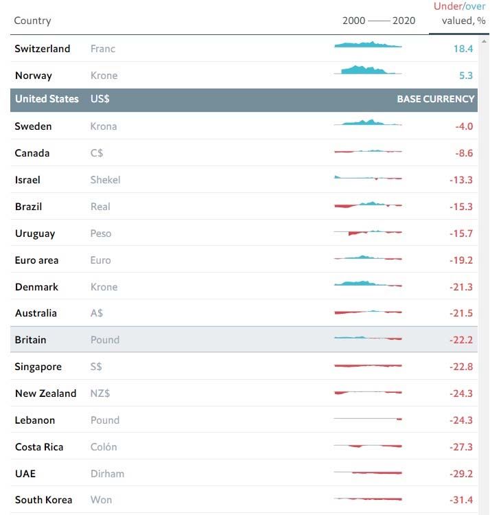
Example (continuation):
Note: It does not matter which currency you borrow in step (1). Recall the
pricing mistake: Bank One undervalues the GBP against the JPY (with
respect to the first two quotes),
        SIJPY/GBP,t = 160 JPY/GBP > SJPY/GBP,t = 140 JPY/GBP

Sketch of Triangular Arbitrage (Key: Buy undervalued GBP with the
overvalued JPY):
(1) Borrow JPY 100
(2) Sell the JPY for GBP (at St = 140 JPY/GBP). Get GBP 0.7143
(3) Sell the GPB for USD (at St = 1.60 USD/GBP). Get USD 1.1429
(4) Sell the USD for JPY (at St = 100 JPY/USD). Get JPY 114.29

         ⇒ Π = JPY 14.29 (14.29% per USD borrowed).

Covered Interest Arbitrage (4 instruments: 2 goods per market and 2
markets)

Open the third section of the WSJ: Brazilian bonds yield 10% and Japanese
bonds 1%.

Q: Why wouldn't capital flow to Brazil from Japan?
A: FX risk: Once JPY are exchanged for BRL (Brazilian reals), there is no
guarantee that the BRL will not depreciate against the JPY.

        ⇒ The only way to avoid this FX risk is to be covered with a
                  forward FX contract.

                                                                             4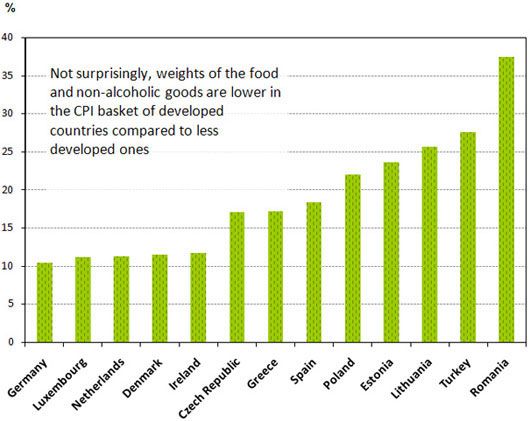
Intuition: Suppose today, at t=0, we have the following data:
iJPY = 1% for 1 year (T=1 year)
iBRL = 10% for 1 year (T=1 year)
St = .025 BRL/JPY

Carry Trade: A strategy to take “advantage” of interest rate differentials:
Today (time t=0), we do the following:
(1) Borrow JPY 1000 at 1% for 1 year.
        (At T=1 year, we will need to repay JPY 1010.)
(2) Convert to BRL at .025 BRL/JPY. Get BRL 25.
(3) Deposit BRL 25 at 10% for 1 year.
        (At T=1 year, we will receive BRL 27.50.)

At time T=1 year, we do the final step:
(4) Exchange BRL 27.50 for JPY at ST=1-year
        ⇒ Π = BRL 27.50 / ST=1-year – JPY 1010

Problem with this strategy: It is risky ⇒ today (t=0), ST=1-year is unknown

Suppose at t=0, a bank offers Ft,1-year = .026 BRL/JPY.

Then, at time T=1 year, we do the final step:
(4’) Exchange BRL 27.50 for JPY at .026 BRL/JPY.
        ⇒ We get JPY 1057.6923 (= BRL 27.50/.026 BRL/JPY).
        ⇒ П = JPY 1057.6923 – JPY 1010 = JPY 47.8
            or 4.78% per JPY borrowed.

Now, instead of borrowing JPY 1000, we will try to borrow JPY 10 billion
(and make a JPY 478M profit) or more.

Obviously, no bank will offer a .026 BRL/JPY forward contract!

        ⇒ Banks will offer Ft,1-year contracts that produce П ≤ 0.

                                                                              5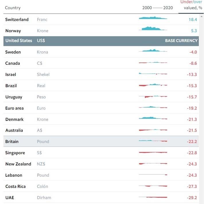
Interest Rate Parity Theorem
Q: How do banks price FX forward contracts?
A: In such a way that arbitrageurs cannot take advantage of their quotes.
To price a forward contract, banks consider covered arbitrage strategies.
Notation:
id = domestic nominal T days interest rate (annualized).
if = foreign nominal T days interest rate (annualized).
St = time t spot rate (direct quote, for example USD/GBP).
Ft,T = forward rate for delivery at date T, at time t.
Note: In developed markets (like the US), all interest rates are quoted on
annualized basis.
Now, consider the following (covered) strategy:
1. At t=0, borrow from a foreign bank 1 unit of a FC for T days.
At time T, We pay the foreign bank FC: (1+if * T/360).
2. At t=0, exchange FC 1 = DC St.
3. Deposit DC St in a domestic bank for T days.
At time T, we receive DC: St(1+id * T/360).
4. At t=0, buy a T-day forward contract to exchange DC for FC at a Ft,T.
At time T, we exchange (in DC) St(1+id * T/360) for FC, using Ft,T.
We get FC: St(1+id * T/360)/Ft,T.
This strategy will not be profitable if, at time T, what we receive in FC is
less or equal to what we have to pay in FC. That is, arbitrage will force:
St (1 + id * T/360)/Ft,T = (1 + if * T/360).
S t (1 i d x T/360)
Solving for Ft,T, we get: Ft, T
(1 i f x T/360)
6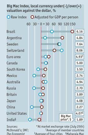
(1 i d x T/360)
Ft,T S t
(1 i f x T/360)
This equation represents the Interest Rate Parity Theorem (IRPT or just IRP).
It is common to use the following linear IRPT approximation:
Ft,T St [1 + (id – if) * T/360].
This linear approximation is quite accurate for small differences in (id – if).
Example: Using IRPT.
St = 106 JPY/USD.
id=JPY = .034.
if=USD = .050.
T = 1 year
Ft,1-year = 106 JPY/USD * (1+.034)/(1+.050) = 104.384 JPY/USD.
Using the linear approximation:
Ft,1-year 106 JPY/USD * (1 – .016) = 104.304 JPY/USD.
Example 1: Violation of IRPT at work.
St = 106 JPY/USD.
id=JPY = .034.
if=USD = .050.
Ft,1-year-IRP = 106 JPY/USD x (1 – .016) = 104.304 JPY/USD.
Suppose Bank A offers: FAt,1-year= 100 JPY/USD.
FAt,1-year= 100 JPY/USD < Ft,1-year-IRP (a pricing mistake!)
The forward USD is undervalued against the JPY.
Let’s take advantage of Bank A’s mistake: Buy USD forward.
Sketch of a covered arbitrage strategy:
(1) Borrow USD 1 from a U.S. bank for one year at 5%.
(2) Exchange the USD for JPY at St = 106 JPY/USD.
(3) Deposit the JPY in a Japanese bank at 3.4%.
(4) Cover. Buy USD forward (Sell forward JPY) at FAt,1-yr= 100 JPY/USD
7
Example 1 (continuation):
t=today T = 1 year
Borrow 1 USD 5% USD 1.05
Deposit JPY 106 3.4% JPY 109.6
Cash flows at time T = 1 year,
(i) We get: JPY 106 * (1+.034)/(100 JPY/USD) = USD 1.096
(ii) We pay: USD 1 * (1+.05) = USD 1.05
П = USD 1.096 – USD 1.05 = USD .046
That is, after one year, the U.S. investor realizes a risk-free profit of USD
.046 per USD borrowed (4.6% per unit borrowed).
Note: Arbitrage will force Bank A’s quote to quickly converge to
Ft,1-yr-IRP = 104.3 JPY/USD. 
Example 2: Violation of IRPT 2.
Now, suppose Bank X offers: FXt,1-year= 110 JPY/USD.
FXt,1-year= 110 JPY/USD > Ft,1-year-IRP (a pricing mistake!)
The forward USD is overvalued against the JPY.
Let’s take advantage of Bank X’s overvaluation: Sell USD forward.
Sketch of a covered arbitrage strategy:
(1) Borrow JPY 1 for one year at 3.4%.
(2) Exchange the JPY for USD at St = 106 JPY/USD
(3) Deposit the USD at 5% for one year.
(4) Cover. Sell USD forward (Buy forward JPY) at FXt,1-yr= 110 JPY/USD.
Cash flows at T=1 year:
(i) We get: USD 1/106 * (1+.05) * (110 JPY/USD) = JPY 1.0896
(ii) We pay: JPY 1 * (1+.034) = JPY 1.034
П = JPY 1.0896 – JPY 1.034 = JPY .0556 (or 5.56% per JPY borrowed)
8
The Forward Premium and the IRPT
Reconsider the linearized IRPT. That is,
Ft,T St [1 + (id – if) * T/360].
A little algebra gives us:
(Ft,T - St)/St * 360/T (id – if)
Let T=360. Then,
p id – if.
Note: p measures the annualized % gain/loss of buying FC spot and selling
it forward. We think of p + if as the annualized return from borrowing DC
and investing in FC (covered) for T days. The opportunity cost of doing
this is id.
Equilibrium: p exactly compensates (id – if) → No arbitrage
→ No capital flows.
Equilibrium: p id - if. IPR Line
IRP Line
id -if
(id - if) > p
(Capital inflows)
45º
B p (forward premium)
Example: Go back to Example 1
p = [(Ft,T - St)/St] * 360/T = [(100 – 106)/106] * 360/360 = - 0.0566
p = - 0.0566 < (id - if) = - 0.016 Arbitrage (pricing mistake!)
Capital flows to DC country
9
Under the linear approximation, we have the IRP Line:
IRP Line
i d - if
B (Capital inflows)
- Example 1
(Capital outflows)
A
- Example 2
45º
p (forward premium)
Consider point A (like in Example 2): p > id – if (or p + if > id),
Borrow at id & invest at if: Capital fly to the foreign country!
Intuition: What an investor pays to finance the foreign investment, id, is
more than compensated by the high forward premium, p, plus if .
IRPT: Assumptions
Behind steps (1) to (4), we have implicitly assumed:
(1) Funding is available. Step (1) can be executed.
(2) Free capital mobility. Step (2) and later (4) can be implemented.
(3) No default/country risk. Step (3) and (4) are safe.
(4) No significant frictions. Typical examples: transaction costs & taxes. Small
transactions costs are OK, as long as they do not impede arbitrage.
We are also implicitly assuming that the forward contract for the desired
maturity T is available. This may not be true.
In general, the forward market is liquid for short maturities (up to 1 year).
For many currencies, say from emerging market, the forward market may
be liquid for much shorter maturities (up to 30 days).
10IRPT with Bid-Ask Spreads
Exchange rates and interest rates are quoted with bid-ask spreads.
Consider a trader in the interbank market:
She buys FC (Sask,t, Fask,t) or borrows at the other party's ask quote (iask).
She sells FC (Sbid,t, Fbid,t) or lends at the bid price (ibid).
There are two roads to take for arbitrageurs:
(1) Borrow domestic currency (at iask,d).
(2) Borrow foreign currency (at iask,f).
• Bid’s Bound: Borrow Domestic Currency
(1) A trader borrows DC 1 at time t=0, and repays 1+iask,d at time=T.
(2) Using the borrowed DC 1, she buys FC spot at Sask,t , getting (1/Sask,t).
(3) She deposits the FC at the foreign interest rate, ibid,f.
(4) She sells the FC forward for T days at Fbid,t,T
This strategy would yield, in terms of DC:
(1/Sask,t) (1+ibid,f) Fbid,t,T.
In equilibrium, this strategy should yield no profit. That is,
(1/Sask,t) (1+ibid,f) Fbid,t,T (1+iask,d).
Solving for Fbid,t,T,
Fbid,t,T Sask,t [(1+iask,d)/(1+ibid,f)] = Ubid.
11• Ask’s Bound: Borrow Foreign Currency
(1) The trader borrows FC 1 at time t=0, and repay 1+iask,f.
(2) Using the borrowed FC 1, she sells the FC spot for Sbif,t units of DC.
(3) She deposits the DC at the domestic interest rate, ibid,d.
(4) She buys the FC forward for T days at Fask,t,T
Following a similar procedure as the one detailed above, we get:
Fask,t,T Sbid,t [(1+ibid,d)/(1+iask,f)] = Lask.
Example: IRPT bounds at work.
Data: St = 1.6540 - 1.6620 USD/GBP
iUSD = 7¼-½,
iGBP = 8⅛ – ⅜,
Ft,one-year= 1.6400 - 1.6450 USD/GBP.
Check if there is an arbitrage opportunity (we need to check the bid’s
bound and ask’s bound).
i) Bid’s bound covered arbitrage strategy:
1) Borrow USD 1 at 7.50% for 1 year
Repay USD 1.07500 in 1 year.
2) Convert to GBP & get GBP 1/1.6620 = GBP 0.6017
3) Deposit GBP 0.6017 at 8.125%
4) Sell GBP forward at 1.64 USD/GBP
we get (1/1.6620) * (1 + .08125) * 1.64 = USD 1.06694
No arbitrage: For each USD borrowed, we lose USD .00806.
12Example (continuation):
ii) Ask’s bound covered arbitrage strategy:
1) Borrow GBP 1 at 8.375% for 1 year we will repay GBP 1.08375.
2) Convert to USD & get USD 1.6540
3) Deposit USD 1.6540 at 7.250%
4) Buy GBP forward at 1.645 USD/GBP
we get 1.6540 * (1 + .07250) * (1/1.6450) = GBP 1.07837
No arbitrage: For each GBP borrowed, we lose GBP 0.0054.
Note: The bid-ask forward quote is consistent with no arbitrage. That is,
the forward quote is within the IRPT bounds. Check:
Ubid = Sask,t[(1+iask,d)/(1+ibid,f)] = 1.6620 * [1.0750/1.08125]
= 1.6524 USD/GBP Fbid,t,T = 1.6400 USD/GBP.
Lask = Sbid,t[(1+ibid,d)/(1+iask,f)] = 1.6540 * [1.0725/1.08375]
= 1.6368 USD/GBP Fask,t,T = 1.6450 USD/GBP. 
Synthetic Forward Rates
A trader is not able to find a specific forward currency contract.
This trader might be able to replicate the forward contract using a spot
currency contract combined with borrowing and lending.
This replication is done using the IRP equation.
Example: Replicating a USD/GBP 10-year forward contract.
iUSD,10-yr = 6%
iGBP,10-yr = 8%
St = 1.60 USD/GBP
T = 10 years.
Ignoring transactions costs, she creates a 10-year (implicit quote) forward
quote:
1) Borrow USD 1 at 6% for 10 years
2) Convert to GBP at 1.60 USD/GBP
3) Invest in GBP at 8% for 10 years
13Transactions to create a 10-year (implicit) forward quote:
1) Borrow USD 1 at 6%
2) Convert to GBP at 1.60 USD/GBP (GBP 0.625)
3) Invest in GBP at 8%
Cash flows in 10 years:
(1) Trader will receive GBP 1.34933 (=1.0810/1.60)
(2) Trader will have to repay USD 1.79085 (= 1.0610)
We have created an implicit forward quote:
USD 1.79085/ GBP 1.34933 = 1.3272 USD/GBP. 
Or
Ft,10-year = St [(1+id,10-year)/(1+if,10-year)]10
= 1.60 USD/GBP [1.06/1.08]10 = 1.3272 USD/GBP. 
Synthetic forward contracts are very useful for exotic currencies.
IRPT: Evidence
Starting from Frenkel and Levich (1975), there is a lot of evidence that
supports IRPT.
Taylor (1989): Strong support for IRPT using 10’ intervals.
Akram, Rice and Sarno (2008, 2009): Using tick-by-tick data, show that
there are short-lived (from 30 seconds up to 4 minutes) departures from
IRP, with a potential profit range of 0.0002-0.0006 per unit.
Overall, the short-lived nature and small profit range point out to a fairly
efficient market, with the data close to the IRPT line.
But, there are situations where we see significant deviations from the IRPT
line. These situations reflect violations of IRPT’s assumptions
For example, during the 2007-2008 financial crisis there were violations of
IRPT. Probable cause: funding constraints –Step (1) in trouble!
14IRPT: Evidence
May 2009: (-.0154,-.0005).
The Behavior of FX Rates
• Fundamentals that affect FX Rates: Formal Theories
- Inflation rates differentials (IUSD - IFC) PPP
- Interest rate differentials (iUSD - iFC) IFE
- Income growth rates (yUSD - yFC) Monetary Approach
- Trade flows Balance of Trade
- Other: trade barriers, expectations, taxes, etc.
• Goal 1: Explain St with a theory, say T1. Then, StT1 = f(.)
Different theories can produce different f(.)’s.
Evaluation: How well a theory match the observed behavior of St.
• Goal 2: Eventually, produce a formula to forecast St+T = f(Xt) E[St+T].
15• We want to have a theory that can match the observed St. It is not realistic
to expect a perfect match, so we ask the question: On average, is St ≈ StT1 ?
Or, alternatively, is E[St] = E[StT1]?
MXN/USD Level: 1989-2018
25
20
15
10
5
0
12/1/1989
12/1/1990
12/1/1991
12/1/1992
12/1/1993
12/1/1994
12/1/1995
12/1/1996
12/1/1997
12/1/1998
12/1/1999
12/1/2000
12/1/2001
12/1/2002
12/1/2003
12/1/2004
12/1/2005
12/1/2006
12/1/2007
12/1/2008
12/1/2009
12/1/2010
12/1/2011
12/1/2012
12/1/2013
12/1/2014
12/1/2015
12/1/2016
12/1/2017
12/1/2018
• Like many macroeconomic series, exchange rates have a trend –in
statistics the trends in macroeconomic series are called stochastic trends. It is
better to try to match changes, not levels.
• Now, the trend is gone. Our goal is to explain st, the percentage change
in St. (Notation: Many times st = ef,t).
MXN/USD Changes: 1990-2018
0.5
0.4
0.3
0.2
0.1
0
‐0.1
‐0.2
1/1/1990
3/1/1991
5/1/1992
7/1/1993
9/1/1994
11/1/1995
1/1/1997
3/1/1998
5/1/1999
7/1/2000
9/1/2001
11/1/2002
1/1/2004
3/1/2005
5/1/2006
7/1/2007
9/1/2008
11/1/2009
1/1/2011
3/1/2012
5/1/2013
7/1/2014
9/1/2015
11/1/2016
1/1/2018
• Our goal is to explain st, the percentage change in St. Again, we will try to
see if the model we are using, say T1, matches, on average, the observed
behavior of st. For example, is E[st] = E[stT1]?
16• We will use statistics to formally tests theories.
• Let’s look at the distribution of st for the MXN/USD –in this case, we
look at monthly percentage changes from 1990-2018.
MXN/USD Changes: Frequency
140
120
100
80
60
40
20
0
-0.12 -0.1 -0.08 -0.06 -0.04 -0.02 0 0.02 0.04 0.06 0.08 0.1 0.12 0.16 More
• The average (“usual”) monthly percentage change is a 0.64% appreciation
of the USD (annualized 8% change). The SD is 3.92% (13.6% annualized).
• These numbers are the ones to match with our theories for St. A good
theory should predict an average annualized change close to 8% for st.
• Descriptive stats for st for the JPY/USD and the MXN/USD.
JPY/USD USD/MXN
Mean -0.0026 0.0064
Standard Error 0.0014 0.0026
Median -0.0004 0.0025
Mode 0 0
Standard Deviation 0.0318 0.0392
Sample Variance 0.0010 0.0021
Kurtosis 1.6088 49.8443
Skewness -0.2606 4.8432
Range 0.2566 0.5812
Minimum -0.1474 -0.1282
Maximum 0.1092 0.4530
Sum -1.2831 -2.7354
Count 491 349
• Developed currencies: less volatile, with smaller means/medians.
17Purchasing Power Parity (PPP)
Purchasing Power Parity (PPP)
PPP is based on the law of one price (LOOP): Goods, once denominated
in the same currency, should have the same price.
If they are not, then some form of arbitrage is possible.
Example: LOOP for Oil.
Poil-USA = USD 80.
Poil-SWIT = CHF 160.
StLOOP = USD 80 / CHF 160 = 0.50 USD/CHF.
If St = 0.75 USD/CHF Oil in Switzerland is more expensive –once
denominated in USD- than in the US:
Poil-SWIT (USD) = CHF 160 * 0.75 USD/CHF = USD 120 > Poil-USA
Example (continuation):
St = 0.75 > StLOOP (LOOP is not holding)
Trading strategy:
(1) Buy oil in the US at Poil-USA = USD 80.
(2) Export oil to Switzerland
(3) Sell US oil in Switzerland at Poil-SWIT = CHF 160.
(4) Sell CHF/buy USD at then St.
This trading strategy, exporting US of oil to Switzerland, will affect prices:
Poil-USA↑; Poil-SWIT↓; & St↓ StLOOP ↑ (= Poil-USA↑/Poil-SWIT↓)
St ⟺ StLOOP (convergence). 
18Example (continuation):
LOOP Notes :
⋄ LOOP gives an equilibrium exchange rate.
Equilibrium will be reached when there is no trade
in oil (because of pricing mistakes). That is, when
the LOOP holds for oil.
⋄ LOOP is telling what St should be (in equilibrium). Not what St is in the
market today.
⋄ Using the LOOP we have generated a model for St. We’ll call this model,
when applied to many goods, the PPP model.
Problem: There are many traded goods in the economy.
Solution: Use baskets of goods.
PPP: The price of a basket of goods should be the same across countries,
once denominated in the same currency. That is, USD 1 should buy the
same amounts of goods here (in the U.S.) or in Colombia.
19• A popular basket: The CPI basket. In the US, the basket typically reported
is the CPI-U, which represents the spending patterns of all urban consumers
and urban wage earners and clerical workers. (87% of the total U.S. population).
• U.S. basket weights:
Food
US: CPI-U Weights
Energy
12% 14%
Food Household Furnishings
Apparel
7%
New vehicles
10%
Used cars and trucks
7%
Recreation
3%
Housing
4% Health care
3%
2%
Housing 6%
32%
• A potential problem with the CPI basket: The composition of the index
(the weights and the composition of each category) may be very different.
• For example, the weight of the food category changes substantially as the
income level increases.
20Absolute version of PPP: The FX rate between two currencies is simply
the ratio of the two countries' general price levels:
StPPP = Domestic Price level / Foreign Price level = Pd / Pf
Example: Law of one price for CPIs.
CPI-basketUSA = PUSA = USD 755.3
CPI-basketSWIT = PSWIT = CHF 1,241.2
StPPP = USD 755.3/CHF 1,241.2 = 0.6085 USD/CHF.
If St 0.6085 USD/CHF, there will be trade of the goods in the basket
between Switzerland and US.
Suppose St = 0.70 USD/CHF > StPPP.
Then, PSWIT (in USD) = CHF 1,241.2 * 0.70 USD/CHF
= USD 868.70 > PUSA = USD 755.3
Example (continuation): (disequilibrium: St = 0.70 USD/CHF > StPPP)
PSWIT (in USD) = CHF 1241.2 * 0.70 USD/CHF
= USD 868.70 > PUSA = USD 755.3
Potential profit: USD 868.70 – USD 755.3 = USD 93.40
Traders will do the following pseudo-arbitrage strategy:
1) Borrow USD
2) Buy the CPI-basket in the US
3) Sell the CPI-basket, purchased in the US, in Switzerland.
4) Sell the CHF/Buy USD
5) Repay the USD loan, keep the profits.
Note: “Equilibrium forces” at work:
2) PUSA ↑ & 3) PSWIT ↓ (=> StPPP↑ = PUSA ↑ / PSWIT ↓)
4) St ↓. St ⟺ StPPP (converge) 
21• Real v. Nominal Exchange Rates
The absolute version of the PPP theory is expressed in terms of St, the
nominal exchange rate.
We can modify the absolute version of the PPP relationship in terms of the
real exchange rate, Rt. That is,
R t = St P f / P d = 1
Rt allows us to compare prices, translated to DC:
If Rt > 1, foreign prices (translated to DC) are more expensive
If Rt = 1, prices are equal in both countries –i.e., PPP holds!
If Rt < 1, foreign prices are cheaper
Economists associate Rt > 1 with a more efficient domestic economy.
Example: Suppose a basket’s –the Big Mac– cost in Switzerland and in the
U.S. is CHF 6.50 and USD 4.93, respectively.
Pf = CHF 6.50
Pd = USD 4.93
St = 0.9908 USD/CHF => Pf (in USD) = USD 6.44 > Pd
Rt = St PSWIT / PUS = 0.9908 USD/CHF * CHF 6.50/USD 4.93 = 1.3065.
Taking the Big Mac as our basket, the U.S. is more competitive than
Switzerland. Swiss prices are 30.65% higher than U.S. prices, after taking
into account the nominal exchange rate.
To bring the economy to equilibrium –no trade in Big Macs-, we expect the
USD to appreciate against the CHF.
According to PPP, the USD is undervalued against the CHF.
=> Trading Signal: Buy USD/Sell CHF. 
22• The Big Mac (“Burgernomics,” popularized by The Economist) has become
a popular basket for PPP calculations. Why?
1) It is a standardized, common basket: beef, cheese, onion, lettuce, bread,
pickles and special sauce. It is sold in over 120 countries.
Big Mac (Sydney) Big Mac (Tokyo)
2) It is very easy to find out the price.
3) It turns out, it is correlated with more complicated common baskets, like
the PWT (Penn World Tables) based baskets.
Using CPI baskets may not work well for absolute PPP. CPI baskets can be
very different. In theory, traders can exploit the price differentials in BMs.
The Economist's Big Mac Index
• In the previous example, Swiss traders can import US BMs.
From UH (US) to
Rapperswill (CH)
• Not realistic. But, the components of a BM are internationally traded.
LOOP suggests that prices of components should be similar in all markets.
The Economist reports the real exchange rate: Rt = StPBigMac,f/PBigMac,d.
For example, in 2020, for the British pound (GBP):
Rt = [GBP 3.39 * 1.2987 USD/GBP] / USD 5.67 = 0.7764
(22.36% overvaluation)
23Example: (The Economist’s) Big Mac Index in 2020.
StPPP = PBigMac,d / PBigMac,f
(The Economist reports Rt – 1 = StPBigMac,f/PBigMac,d – 1).
Rt > 1
Rt < 1
Example: (The Economist’s) Big Mac Index in January 2020.
24Example: Big Mac Index - Rt Changes over time in 2000-2016.
CHF/USD
BRL/USD
But, Rt departures from 1, can be very persistent.
Example: Iphone 6 (March 2015, taken from seekingalpha.com).
Rt = StPIPhone,f/PIPhone,d (d=US) Rt=1 under Absolute PPP
25• Empirical Evidence: Simple informal test:
Test: If Absolute PPP holds Rt = 1.
In the Big Mac example, PPP does not hold for the majority of countries.
Several tests of the absolute version have been performed: Absolute
version of PPP, in general, fails (especially, in the short run).
• Absolute PPP: Qualifications
(1) PPP emphasizes only trade and price levels. Political/social factors (instability,
wars), financial problems (debt crisis), etc. are ignored.
(2) Implicit assumption: Absence of trade frictions (tariffs, quotas, transactions
costs, taxes, etc.).
Q: Realistic? On average, transportation costs add 7% to the price of U.S.
imports of meat and 16% to the import price of vegetables. Many products
are heavily protected, even in the U.S. For example, peanut imports are
subject to a tariff as high as 163.8%. Also, in the U.S., tobacco usage and
excise taxes add USD 5.85 per pack.
• Absolute PPP: Qualifications
Some everyday goods protected in the U.S.:
- European Roquefort Cheese, cured ham, mineral water (100%)
- Paper Clips (as high as 126.94%)
- Canned Tuna (as high as 35%)
- Synthetic fabrics (32%)
- Sneakers (48% on certain sneakers)
- Japanese leather (40%)
- Peanuts (shelled 131.8%, and unshelled 163.8%).
- Brooms (quotas and/or tariff of up to 32%)
- Chinese tires (35%)
- Trucks (25%) & cars (2.5%)
Some Japanese protected goods:
- Rice (778%)
- Beef (38.5%, but can jump to 50% depending on volume).
- Sugar (328%)
- Powdered Milk (218%)
26• Absolute PPP: Qualifications
(3) PPP is unlikely to hold if Pf and Pd represent different baskets. This is why
the Big Mac is a popular choice.
(4) Trade takes time (contracts, information problems, etc.).
(5) Internationally non-traded (NT) goods –i.e. haircuts, home and car repairs,
hotels, restaurants, medical services, real estate. The NT good sector is big:
50%-60% of GDP (big weight in CPI basket).
Then, in countries where NT goods are relatively high, the CPI basket will
also be relatively expensive. Thus, PPP will find these countries' currencies
overvalued relative to currencies in low NT cost countries.
Note: In the short-run, we will not take our cars to Mexico to be repaired,
but in the long-run, resources (capital, labor) will move. We can think of
the over-/under-valuation as an indicator of movement of resources.
• Absolute PPP: Qualifications
The NT sector also has an effect on the price of traded goods. For
example, rent and utilities costs affect the price of a Big Mac: 25% of Big
Mac due to NT goods.
• Empirical Fact
Price levels in richer countries are consistently higher than in poorer ones.
This fact is called the Penn effect. Many explanations, the most popular: The
Balassa-Samuelson (BS) effect.
• Borders Matter
You may look at the Big Mac Index and think: “No big deal: there is also a
big dispersion in prices within the U.S., within Texas, and, even, within
Houston!” It is true that prices vary within the U.S.
For example, in 2015, the price of a Big Mac (and Big Mac Meal) in New
York was USD 5.23 (USD 7.45), in Texas as USD 4.39 (USD 6.26) and in
Mississippi was USD 3.91 (USD 5.69).
27But, borders play a role, not just distance!
Engel and Rogers (1996) computed the variance of LOOP deviations for
city pairs within the U.S., within Canada, and across the border.: Distance
between cities within a country matter, but the border effect is significant.
To explain the difference between prices across the border using the
estimate distance effects within a country, they estimate the U.S.-Canada
border should have a width of 75,000 miles!
This huge estimate has been revised downward in subsequent studies, but a
large positive border effect remains.
• Balassa-Samuelson Effect
Labor costs affect all prices. We expect average prices to be cheaper in poor
countries than in rich ones because labor costs are lower.
This is the so-called Balassa-Samuelson effect: Rich countries have higher
productivity and, thus, higher wages in the traded-goods sector than poor
countries do. But, firms compete for workers.
Then, wages in NT goods and services are also higher Overall prices are
lower in poor countries.
28• For example, in 2000, a typical McDonald’s worker in the U.S. made USD
6.50/hour, while in China made USD 0.42/hour.
• The Balassa-Samuelson effect implies a positive correlation between PPP
exchange rates (overvaluation) and high productivity countries.
• Incorporating the Balassa-Samuelson effect into PPP:
1) Estimate a regression: Big Mac Prices against GDP per capita.
BigMac_Price_(in USD)t = α + β GDP_per_capitat + εt
Switzerland
Brazil
+ β GDP_per_capitat
Hong Kong
29• Incorporating the Balassa-Samuelson effect into PPP:
Same regression in July 2011.
• Incorporating the Balassa-Samuelson effect into PPP:
2) Compute fitted Big Mac Prices (GDP-adjusted Big Mac Prices), along the
regression (red) line. Use the difference between GDP-adjusted Big Mac Prices
and actual prices (the white/blue dots) to estimate GDP-adjusted PPP
over/under-valuation.
30Example: Raw vs GDP-Adjusted Big Mac Index in 2019.
• Pricing-to-Market
Krugman (1987) offers an alternative explanation for the strong positive
relationship between GDP and price levels: Pricing-to-market –i.e., price
discrimination.
Based on price elasticities, producers discriminate: the same exact good is
sold to rich countries (lower price elasticity) at higher prices than to poorer
countries (higher price elasticity).
Alessandria and Kaboski (2008) report that U.S. exporters, on average, charge
the richest country a 48% higher price than the poorest country.
Again, pricing-to-market struggles to explain why PPP does not hold among
developed countries with similar incomes. For example, Baxter and Landry
(2012) report that IKEA prices deviate 16% from the LOOP in Canada, but
only 1% in the U.S.
31Main PPP criticism
Absolute PPP does not incorporate transaction costs and frictions. Relative
PPP allows for fixed transaction costs and frictions (say, a fixed USD
amount).
Relative PPP
The rate of change in the prices of products should be similar when
measured in a common currency (as long as trade frictions are unchanged):
S tT S t (1 I d )
s tPPP
,T 1 (Relative PPP)
St (1 I f )
where,
If = foreign inflation rate from t to t+T;
Id = domestic inflation rate from t to t+T.
Note: st,TPPP is an expectation; what we expect to happen in equilibrium.
• Linear approximation: st,TPPP (Id - If) one-to-one relation
Relative PPP
• Linear approximation: st,TPPP (Id - If) one-to-one relation
Example: From t=0 to t=1, prices increase 10% in Mexico relative to
prices in Switzerland. Then, St should also increase 10%.
If S0 = 9 MXN/CHF S1PPP = E[S1] = 9.9 MXN/CHF.
Suppose S1= 10.2 MXN/CHF > 9.9 MXN/CHF,
According to Relative PPP, the CHF is overvalued. 
Notation: E[S1] = Expected value of S1 (according to a model), a forecast.
32Example: Forecasting St (USD/ZAR) using PPP (ZAR=South Africa).
It’s 2013. You have the following information:
CPIUS,2013 = 104.5,
CPISA,2013 = 100.0,
S2013 = .2035 USD/ZAR.
You are given the 2014 CPI’s forecast for the U.S. and SA:
E[CPIUS,2014] = 110.8
E[CPISA,2014] = 102.5.
You want to forecast S2014 using the relative (linearized) version of PPP.
E[IUS-2014] = (110.8/104.5) - 1 = .06029
E[ISA-2014] = (102.5/100) - 1 = .025
E[S2014] = S2013 * (1 + st,TPPP ) = S2013 * (1 + E[IUS]- E[ISA])
= .2035 USD/ZAR * (1 + .06029 - .025) = .2107 USD/ZAR.
Under the linear approximation, we have PPP Line
Id - If
PPP Line
B (FC appreciates)
A (FC depreciates)
45º
sT (DC/FC)
Look at point A: sT > Id - If,
Priced in FC, the domestic basket is cheaper
pseudo-arbitrage (trade) against foreign basket FC depreciates
33• Relative PPP: Implications
(1) Under relative PPP, Rt remains constant (it can be different from 1!).
(2) Relative PPP does not imply that St is easy to forecast.
(3) Without relative price changes, an MNC faces no real operating FX risk
(as long as the firm avoids fixed contracts denominated in FC).
• Relative PPP: Absolute versus Relative
- Absolute PPP compares price levels.
Under Absolute PPP, prices are equalized across countries: "A mattress costs
GBP 200 (= USD 320) in the U.K. and BRL 800 (=USD 320) in Brazil.“
- Relative PPP compares price changes.
Under Relative PPP, exchange rates change by the same amount as the
inflation rate differential (original prices can be different): “U.K. inflation was
2% while Brazilian inflation was 8%. Meanwhile, the BRL depreciated 6% against the
GBP. Then, relative cost comparison remains the same.”
• Relative PPP is a weaker condition than Absolute PPP: Rt can be
different from 1.
• Relative PPP: Testing
Key: On average, what we expect to happen, st,TPPP, should happen, st,T.
On average: st,T st,TPPP Id – If
or E[st,T] = E[st,TPPP ] E[ Id – If ]
A linear regression is a good framework to test theories. Recall,
st,T = (St+T - St)/St = α + β (Id - If )t+T + εt+T,
where ε: regression error. That is, E[εt+T]=0.
Then, E[st,T ] = α + β E[(Id - If )t+T] + E[εt+T] = α + β E[st,TPPP ]
E[st,T] = α + β E[st,TPPP ]
For Relative PPP to hold, on average, we need α=0 & β=1.
34• Relative PPP: General Evidence
Under Relative PPP: st,T Id – If
1. Visual Evidence
Plot (IJPY-IUSD) against st(JPY/USD), using monthly data 1971-2015.
Test: Is there a 45° line?
st,T
IJPY-IUSD
No 45° line Visual evidence rejects PPP.
• Relative PPP: General Evidence
Under Relative PPP: st,T Id – If
1. Visual Evidence
Plot (IGBP-IUSD) against st(GBP/USD), using monthly data 1971-2017.
Test: Is there a 45° line?
Relative PPP (GBP/USD)
0.04
0.03
0.02
(Igbp - Iusd)
0.01
0
-0.15 -0.1 -0.05 0 0.05 0.1 0.15 0.2
-0.01
-0.02
s_t (GBP/USD)
No 45° line Visual evidence rejects PPP.
35• Relative PPP: General Evidence
1. Visual Evidence
Test: Is Rt 1? (Actually, constant, under Relative PPP)
Real Exchange Rate: JPY/USD
3.5
3
2.5
2
1.5
1
0.5
0
1/1/1971
6/1/1972
11/1/1973
4/1/1975
9/1/1976
2/1/1978
7/1/1979
12/1/1980
5/1/1982
10/1/1983
3/1/1985
8/1/1986
1/1/1988
6/1/1989
11/1/1990
4/1/1992
9/1/1993
2/1/1995
7/1/1996
12/1/1997
5/1/1999
10/1/2000
3/1/2002
8/1/2003
1/1/2005
6/1/2006
11/1/2007
4/1/2009
9/1/2010
2/1/2012
7/1/2013
12/1/2014
5/1/2016
10/1/2017
Some evidence for mean reversion, though slow, for Rt (average = 1.94).
• Relative PPP: General Evidence (continuation)
In general, we have some evidence for mean reversion for Rt. Loosely
speaking, in the long run, Rt moves around some mean number, which we
associate with the long-run PPP parity. But, the deviations from the long-
run parity are very persistent –i.e., very slow to adjust.
Economists usually report the number of years that a PPP deviation is
expected to decay by 50% (the half-life) is in the range of 3 to 5 years for
developed currencies. Very slow!
• Descriptive Stats
IJPY IUSD IJPY-IUSD st,T (JPY/USD)
Mean 0.0021 0.0033 -0.0012 -0.0015
SD 0.0063 0.0038 0.0061 0.0316
Min -0.0107 -0.0191 -0.0192 -0.1474
Median 0.0010 0.0030 -0.0019 -0.0001
Max 0.0431 0.0177 0.0346 0.1092
362. Statistical Evidence
More formal tests: Regression
st,T = (St+T – St)/St = α + β (Id – If )t+T + εt+T, ε: regression error,
E[εt+T]=0.
The null hypothesis is: H0 (Relative PPP true): α=0 and β=1
H1 (Relative PPP not true): α≠0 and/or β≠1
• Tests: t-test (individual tests on α and β) & F-test (joint test)
(1) Individual test: t-test
t-test = tθ = [θ – θ0]/S.E.(θ)
Statistical distribution: tθ ~ tv (v = N – K =degrees of freedom)
where θ represents α or β ( θ0 = α or β evaluated under H0).
Rule: If |t-test| > |tv,α/2|, reject H0 at the α level.
When v = N – K > 30, t30+,.025 ≈ 1.96 2-sided C.I. α = .05 (5 %)
2. Statistical Evidence
(2) Joint Test: F-test
F-test = {[RSS(H0) – RSS(H1)]/J}/{RSS(H1)/(N-K)}
Statistical distribution: F-test ~ FJ,N-K
J = # of restrictions in H0, (under PPP, J=2: α=0 & β=1)
K = # parameters in model, (under PPP model, K=2: α & β)
N = # of observations,
RSS = Residuals Sum of Squared, εt = et = st – [α β (Id – If )t ].
RSS(H0) = ∑ t (Id,t − If,t) ] 2
RSS(H1) = ∑ (εt)2
Rule: If F-test > FJ,N-K,α, reject at the α level. Usually, α = .05 (5 %)
When N > 300, FJ=2,300+,α=.05 ≈ 3.
37Example: Using monthly Japanese and U.S. data (1/1971-9/2007), we fit
the following regression:
st (JPY/USD) = (St – St-1)/St-1 = α + β (IJAP – IUS) t + εt.
R2 = 0.00525
Standard Error (σ) = .0326
F-stat (slopes=0 –i.e., β=0) = 2.305399 (p-value=0.130)
Observations (N) = 439
Coefficient Stand Err t-Stat P-value
Intercept (α ) 0.00246 0.001587 -1.55214 0.121352
(IJAP – IUS) (β ) -0.36421 0.239873 -1.51835 0.129648
We will test the H0 (Relative PPP true): α=0 & β=1
Two tests: (1) t-tests (individual tests)
(2) F-test (joint test)
Example: Using monthly Japanese and U.S. data (1/1971-9/2007), we fit
the following regression (Observations = 439):
st (JPY/USD) = (St – St-1)/St-1 = α + β (IJAP – IUS) t + εt.
R2 = 0.00525
Standard Error (σ) = .0326
F-stat (slopes=0 –i.e., β=0) = 2.305399 (p-value = 0.130)
F-test (H0: α=0 and β=1): 16.289 (p-value: lower than 0.0001) reject H0 at 5% level
(F2,467,.05= 3.015)
Coefficient Stand Err t-Stat P-value
Intercept (α) -0.00246 0.001587 -1.55214 0.121352
(IJAP – IUS) (β) -0.36421 0.239873 -1.51835 0.129648
Test H0, using t-tests (t437.05=1.96 – Note: when N-K>30, t.05 = 1.96):
tα=0: (-0.00246–0)/0.001587 = -1.55214 (p-value=.12) cannot reject H0.
tβ=1: (-0.36421-1)/0.239873 = -5.6872 (p-value:.00001) reject H0. 
38• PPP Evidence:
⋄ Relative PPP tends to be rejected in the short-run (see example above).
In the long-run, there is debate about its validity. Research shows that
currencies with high inflation rate differentials tend to depreciate.
Real FX (GBP/USD): 1971-2017
1
0.9
0.8
GBP/USD
0.7
0.6
0.5
0.4
0.3
0.2
Feb-71
Feb-73
Feb-75
Feb-77
Feb-79
Feb-81
Feb-83
Feb-85
Feb-87
Feb-89
Feb-91
Feb-93
Feb-95
Feb-97
Feb-99
Feb-01
Feb-03
Feb-05
Feb-07
Feb-09
Feb-11
Feb-13
Feb-15
Feb-17
Some evidence for a mean reverting Rt (average Rt = 0.61). But deviations
can last for years!
• PPP: Rt and St
Mussa (1986) and others shows that Rt is much more variable under a free
float. Rt variability tends to be highly correlated with St variability. Since
1973, when floating exchange rates were adopted, Rt moves like St.
Nominal vs. Real FX (GBP/USD): 1971-2017
1
0.9
0.8
GBP/USD
0.7
0.6
0.5
0.4
Real FX
0.3
Nominal
0.2
Feb-71
Feb-73
Feb-75
Feb-77
Feb-79
Feb-81
Feb-83
Feb-85
Feb-87
Feb-89
Feb-91
Feb-93
Feb-95
Feb-97
Feb-99
Feb-01
Feb-03
Feb-05
Feb-07
Feb-09
Feb-11
Feb-13
Feb-15
Feb-17
As a check to the visual evidence: Volatility(changes in Rt) = 2.94% &
Volatility(changes in St) = 2.90 (correlation = .98). Almost the same!
39Implications: Price levels play a minor role in explaining the movements of
Rt (prices are sticky). Engel (1999) reports that prices seem to be sticky also
for traded-goods.
Possible explanations:
(a) Contracts:
Prices cannot be continuously adjusted due to contracts. In a stable
economy, contracts have longer durations. In high inflation countries
(contracts with shorter duration) PPP deviations are not very persistent.
(b) Mark-up adjustments:
Manufacturers and retailers tend to moderate any increase in their prices in
order to preserve market share. Changes in St are only partially transmitted
or pass-through to import/export prices.
Average ERPT (exchange rate pass-through) is around 50% over one
quarter and 64% over the long run for OECD countries (for the U.S., 25%
in the short-run and 40% over the long run).
(c) Repricing costs (menu costs)
It is expensive to adjust continuously prices; in a restaurant, the repricing
cost is re-doing the menu. For example, Goldberg and Hallerstein (2007)
estimate that the cost of repricing in the imported beer market is 0.4% of
firm revenue for manufacturers and 0.1% of firm revenue for retailers.
(d) Aggregation
Q: Is price rigidity a result of aggregation –i.e., the use of price index?
Empirical work using micro level data –say, same good (exact UPC!) in
Canadian and U.S. grocery stores– show that on average product-level Rt
move closely with St. But, micro level prices show idiosyncratic movements,
mainly unrelated to St: 10% of the deviations from PPP are accounted by St.
• PPP: Puzzle
The fact that no single model of exchange rate determination can
accommodate both the high persistent of PPP deviations and the high
correlation between Rt and St has been called the “PPP puzzle.”
40• PPP: Summary of Empirical Evidence
⋄ Rt and St are highly correlated, Pd (even for traded-goods) tend to be
sticky.
⋄ In the short run, PPP is a very poor model to explain short-term St
movements.
⋄ PPP deviation are very persistent. It takes a long time (years!) to
disappear.
⋄ In the long run, there is some evidence of mean reversion, though very
slow, for Rt. That is, StPPP has long-run information:
Currencies that consistently have high inflation rate differentials –i.e., (Id – If) > 0–
tend to depreciate.
• The long-run interpretation for PPP is the one that economist like and
use. PPP is seen as a benchmark, a figure towards which the current
exchange rate should move.
• Calculating StPPP (Long-Run FX Rate)
Let’s look at the MXN/USD case.
We want to calculate StPPP = Pd,t / Pf,t over time.
(1) Divide StPPP by SoPPP (t=0 is our starting point).
(2) After some algebra,
StPPP = SoPPP * [Pd,t / Pd,o] * [Pf,o/Pf,t]
By assuming SoPPP = So, we plot StPPP over time.
(Note: SoPPP = So assumes that at t=0, the economy was in equilibrium. This
may not be true: Be careful when selecting a base year.)
41Let’s look at the MXN/USD case.
Actual vs Long Run PPP: MXN/USD
30
25
20
15
10
5
PPP MX/US MXN/USD
0
12/1/1987
5/1/1989
10/1/1990
3/1/1992
8/1/1993
1/1/1995
6/1/1996
11/1/1997
4/1/1999
9/1/2000
2/1/2002
7/1/2003
12/1/2004
5/1/2006
10/1/2007
3/1/2009
8/1/2010
1/1/2012
6/1/2013
11/1/2014
4/1/2016
9/1/2017
- In the short-run, StPPP is missing the target, St.
- But, in the long-run, StPPP gets the trend right. (As predicted by PPP, the
high Mexican inflation rates differentials against the U.S., depreciate the
MXN against the USD.)
Another example, let’s look at the JPY/USD case.
Actual vs Long Run PPP: JPY/USD
500
450
400
350
300
250
200
150
100
50
PPP JPY/USD JPY/USD
0
1/1/1971
1/1/1973
1/1/1975
1/1/1977
1/1/1979
1/1/1981
1/1/1983
1/1/1985
1/1/1987
1/1/1989
1/1/1991
1/1/1993
1/1/1995
1/1/1997
1/1/1999
1/1/2001
1/1/2003
1/1/2005
1/1/2007
1/1/2009
1/1/2011
1/1/2013
1/1/2015
1/1/2017
As predicted by PPP, since U.S. inflation rates have been consistently higher
than the Japanese ones, in the long-run, the USD depreciates against the
JPY.
42• PPP Summary of Applications:
⋄ Equilibrium (“long-run”) exchange rates. A CB can use StPPP to determine
intervention bands.
⋄ Explanation of St movements (“currencies with high inflation rate
differentials tend to depreciate”).
⋄ Indicator of competitiveness or under/over-valuation: Rt > 1
FC is overvalued (& Foreign prices are not competitive).
⋄ International GDP comparisons: Instead of using St, StPPP is used to
translate local currencies to USD. For example, Chinese per capita GDP
(World Bank figures, in 2017):
Nominal GDP per capita: CNY 59,670.52;
St = 0.14792 USD/CNY;
- Nominal GDP_cap (USD)= CNY 59,670.52 * 0.1479 USD/CNY= USD 8,827
StPPP = 0.2817 USD/CNY ⇒ “U.S. is 90% more expensive”
- PPP GDP_cap (USD)= CNY 59,670.52 * 0.2817 USD/CNY = USD 16,807.
GDP per capita (in USD) - 2017
Country Nominal PPP
Luxembourg 104,103 103,745
USA 59,532 59,532
Japan 38,428 43,279
Italy 31,953 39,427
Czech Republic 20,368 36,504
Costa Rica 11,631 17,044
Brazil 9,821 15,484
China 8,827 16,807
Lebanon 8,524 14,676
Algeria 4,123 15,275
India 1,937 7,056
Ethiopia 767 1,899
Mozambique 416 1,247
Note: PPP GDP/Nominal GDP = USD 16,807/ USD 8,827 = 1.9040
⇒ “U.S. is 90% more expensive.” 
43International Fisher Effect (IFE)
• IFE builds on the law of one price, but for financial transactions.
• Idea: The return to international investors who invest in money markets
in their home country should be equal to the return they would get if
they invest in foreign money markets once adjusted for currency
fluctuations.
• Exchange rates will be set in such a way that international investors
cannot profit from interest rate differentials --i.e., no profits from carry
trades.
The "effective" T-day return on a foreign bank deposit is:
rf (in DC) = (1 + if * T/360) (1 + st,T) – 1.
• While, the effective T-day return on a home bank deposit is:
rd (in DC) = id * T/360.
• Setting rf (in DC) = rd and solving for st,T = (St+T/St - 1) we get:
(1 i d x T/360)
s IFE
T -1 (This is the IFE)
(1 i f x T/360)
• Using a linear approximation: s , (id – if) * T/360.
• s , represents an expectation. It is the expected change in St from t to
t+T that makes looking for the “extra yield” in international money
markets not profitable.
44• Since IFE gives us an expectation for a future exchange rate –St+T-, if we
believe in IFE we can use this expectation as a forecast.
Example: Forecasting St using IFE.
It’s 2015:I. You have the following information:
S2015:I = 1 .0659 USD/EUR.
iUSD,2015:I = 0.5%
iEUR,2015:I = 1.0%.
T = 1 semester = 180 days.
s, : = [1+ iUSD,2015:I * (T/360)]/[1+ iEUR,2015:I * (T/360)] – 1 =
= [1+.005*(180/360))/[1+.01*(180/360)] – 1 = -0.0024875
E[S2015:II] = S2015:I * (1+ s , : ) = 1.0659 USD/EUR *(1 – 0.0024875)
= 1.06325 USD/EUR
We expect St to change to 1.06325 USD/EUR to compensate for the
lower US interest rates. 
Example (continuation):
E[S2015:II] = S2015:I * (1+ s , : ) = 1.0659 USD/EUR *(1 – 0.0024875)
= 1.06325 USD/EUR
Suppose S2015:II = 1.08 USD/EUR > E[S2015:II] = 1.06325 USD/EUR
According to IFE, EUR is overvalued.
Trading signal: Sell EUR/Buy USD.
Note: we can get to the same result by looking at the changes:
s2015:II = 1.08/1.0659 – 1 = 0.01329 > s , : = -0.0024875.
According to IFE, EUR appreciated more than expected.
That is, EUR is overvalued. 
45• Note: Like PPP, IFE also gives an equilibrium
exchange rate. Equilibrium will be reached when
there is no capital flows from one country to another
to take advantage of interest rate differentials.
IFE: Implications
If IFE holds, the expected cost of borrowing funds is identical across
currencies. Also, the expected return of lending is identical across
currencies.
Carry trades –i.e., borrowing a low interest currency to invest in a high
interest currency- should not be profitable.
If departures from IFE are consistent, investors can profit from them.
Example: Mexican peso depreciated 5% a year during the early 90s.
Annual interest rate differential (iMXN – iUSD) were between 7% and 16%.
The E[st,T] = -5% > sIFEt,T = -7% Pseudo-arbitrage is possible
(The MXN at t+T is overvalued!)
IFE
Suppose we expect Et[st,T] > s t,T to occur in the next T days.
Carry Trade Strategy (USD = DC; we invest in the overvalued currency):
1) Borrow USD funds (at iUSD)
2) Convert to MXN at St
3) Invest in Mexican funds (at iMXN)
4) Wait until T. Convert to USD at St+T –expect: E[St+T]=St*(1+ Et[st,T]).
Expected FX loss = 5% (Et[st,T] = -5%)
Assume (iUSD – iMXN) = -7%. (Say, iUSD = 6%; iMXN = 13%.)
Et[st,T]= -5% > sIFEt= -7% “On average,” strategy (1)-(4) should work.
46Example (continuation):
Expected USD return from MXN investment:
rf (in DC) =(1+ iMXN*T/360)(1+ Et[st,T]) – 1 = (1.13)*(1 –.05) – 1 = 0.074
Payment for USD borrowing: rd = id * T/360 = .06
Expected Profit = E[Π] = 0.074 – .06 = .014 per year
• Overall expected profits ranged from: 1.4% to 11%. 
Note: A carry trade strategy is based on an expectation: Et[st,T] = -5%. It
may or may not occur every time. This is risky!
Example: Risk at work. Fidelity used this uncovered strategy during the
early 90s. In Dec. 94, after the Tequila devaluation of the MXN against the
USD (40% in a month), it lost everything it gained before.
• An IFE driven carry trade differs from covered arbitrage in the final step.
Step 4) involves no coverage. It’s an uncovered strategy. IFE is also called
Uncovered Interest Rate Parity (UIRP).
• UIRP is difficult to test since it involves an expectation (an unobservable).
In general, we test UIRP assuming that on average what we expect occurs.
• Test: UIRP true (no carry trade profits) if st,T (id – if) * T/360.
B (FC undervalued) IFE Line
id - if
A FC overvalued
(Carry trade: Borrow DC)
45º
sT (DC/FC)
471. Visual evidence.
Based on linearized IFE: st,T (id – if) * T/360
Expect a 45 degree line in a plot of ef,T against (id – if)
Example: Plot for the monthly USD/EUR exchange rate (1999-2017)
IFE: USD/EUR
0.05
st 0.04
0.03
0.02
0.01
0
-0.12 -0.07 -0.02 0.03 0.08
-0.01
-0.02
-0.03
-0.04
-0.05
iUSD – iEUR
No 45° line Visual evidence rejects IFE. 
2. Regression evidence
st,T = (St+T – St)/St = α + β (id – if )t + εt, (εt error term, E[εt]=0).
• The null hypothesis is: H0 (IFE true): α=0 and β=1
H0 (IFE not true): α≠0 and/or β≠1
Example: Testing IFE for the USD/EUR with monthly data (1999-2017).
R2 = 0.01331
Standard Error = 0.01815
F-statistic (slopes=0) = 2.6034 (p-value=0.1083)
F-test (α=0 and β=1) = 68.63369 (p-value= lower than 0.0001)
rejects H0 at the 5% level (F2,193,.05=3.05)
Observations = 195
Coefficients Standard Error t Stat P-value
Intercept (α ) 0.000588 0.001935 0.303996 0.76141
(id - if )t (β) -0.05477 0.143501 -0.38169 0.70305
48Let’s test H0, using t-tets (t104,.05 = 1.96) :
tα=0 (t-test for α = 0): (0.000588 – 0)/0.00194 = 0.304
cannot reject H0 at the 5% level.
tβ=1 (t-test for β = 1): (-0.05477 – 1)/0.1435 = -8.045
reject H0 at the 5% level.
Formally, IFE is rejected in the short-run (both the joint test and the t-tests
reject H0). Also, note that β is negative, not positive as IFE expects. 
• IFE is rejected. Then,
Q: Is a “carry trade” strategy profitable?
During the 1999-2017 period, the average monthly (iUSD – iEUR) was:
-0.00164/12= -.00015 stIFE = -0.015% per month (≠0, statistically)
Actual average monthly st(USD/EUR) was .0007 (≈0, statistically speaking)
Et[st] = 0.07% > stIFE = -0.015% (EUR overvalued!)
If we use the regression to derive an expectation, then:
E[sReg,t] = 0.000588 – 0.05477 *(-.00164) = 0.0006 (≈0!)
E[st] = E[sReg,t] = 0.06% > stIFE = -0.015% (EUR overvalued)
Note: Consistent deviations from IFE make carry trades profitable. During
the 1999-2017 period, USD-EUR carry trades should have been profitable.
Carry trade strategy:
1) Borrow USD at iUSD
2) Convert to EUR
3) Deposit EUR at iEUR
4) Wait 30 days and convert back to USD (on average, 0% monthly change)
From 1) + 3), we make 0.015% per month.
From 2) + 3), we lose 0% per month.
Total gain over the whole period: 3.3% (very low!). 
49• IFE: Evidence
No short-run evidence Carry trades work (on average).
Burnside (2008): The average excess return of an equally weighted carry
trade strategy, executed monthly, over the period 1976–2007, was about 5%
per year. (Sharpe ratio twice as big as the S&P500, since annualized
volatility of carry trade returns is much less than that for stocks).
Some long-run support:
“Currencies with high interest rate differentials tend to depreciate.”
(For example, the Mexican peso finally depreciated in Dec. 1994.)
Expectations Hypothesis (EH)
• According to the Expectations hypothesis (EH) of exchange rates:
Et[St+T] = Ft,T.
That is, on average, the future spot rate is equal to the forward rate.
Since expectations are involved, many times the equality will not hold. It
will only hold on average.
Q: Why should this equality hold?
Suppose it does not hold. That means, what people expect to happen at
time T is consistently different from the rate you can set for time T. A
potential profit strategy can be developed that works on average.
50Example: Suppose that over time, investors violate EH.
Data: Ft,180 = 5.17 ZAR/USD.
An investor expects: Et[St+180] = 5.34 ZAR/USD. (A potential profit!)
Strategy for this investor:
1. Buy USD forward at ZAR 5.17
2. In 180 days, sell the USD for ZAR 5.34.
Now, suppose everybody expects Et [St+180] = 5.34 ZAR/USD
Disequilibrium: Everybody buys USD forward (nobody sells USD
forward). And in 180 days, everybody will be selling USD. Prices should
adjust until EH holds.
Since an expectation is involved, sometimes you will have a loss, but, on
average, you will make a profit every time Et[St+T] ≠ Ft,T. 
Expectations Hypothesis: Implications
EH: Et[St+T] = Ft,T → On average, Ft,T is an unbiased predictor of St+T.
Example: Today, it is 2014:II. A firm wants to forecast the quarterly St
USD/GBP. You are given the interest rate differential (in %) and St.
Using IRP you calculate Ft,90: Ft,90 = St [1 + (iUS – iUK)t * T/360].
Data available:
St=2014:II = 1.6883 USD/GBP
(iUS – iUK)t=2014:II = -0.304%.
Then,
Ft,90 = 1.6883 USD/GBP * [1 – 0.00304 * 90/360] = 1.68702 USD/GBP
SFt:2014:III = 1.68702 USD/GBP
According to EH, if a firm forecasts St+T using the forward rate, over time,
will be right on average.
average forecast error Et[St+T - Ft,T] = 0.
51Expectations Hypothesis: Implications
Doing this forecasting exercise each period generates the following
quarterly forecasts and forecasting errors, εt:
Quarter (iUS-iUK) St SFt+90 = Ft,90 εt = St - SFt
2014:II -0.304 1.6883
2014:III -0.395 1.6889 1.68702 0.0019
2014:IV -0.350 1.5999 1.68723 -0.0873
2015:I -0.312 1.5026 1.59850 -0.0959
2015:II -0.415 1.5328 1.50143 0.0314
2015:III -0.495 1.5634 1.53121 0.0322
2015:IV 1.5445 1.56146 -0.0170
Calculation of the forecasting error for 2014:III:
εt=2014:III = 1.6889 – 1.68702 = 0.0019. 
Note: Since (St+T – Ft,T) is unpredictable, expected cash flows associated
with hedging or not hedging currency risk are the same.
Expectations Hypothesis: Evidence
Under EH, Et[St+T] = Ft,T → Et[St+T – Ft,T] = 0
Empirical tests of the EH are based on a regression:
(St+T – Ft,T)/St = α + β Zt + εt,(where E[εt]=0)
where Zt represents any economic variable that might have power to
explain St, for example, (id – if).
H0 (EH true): α = 0 and β = 0. ((St+T – Ft) should be unpredictable!)
H1 (EH not true): α ≠ 0 and/or β ≠ 0.
Usual result: β < 0 (and significant) when Zt= (id – if).
But, the R2 is very low.
52Expectations Hypothesis: IFE (UIRP) Revisited EH: Et[St+T] = Ft,T. Replace Ft,T by IRP, say, linearized version: Et[St+T] ≈ St [1+ (id – if) * T/360]. A little bit of algebra gives: (E[St+T] – St)/St ≈ (id – if) * T/360
You can also read