Assessing biophysical and socio economic impacts of climate change on regional avian biodiversity - Nature
←
→
Page content transcription
If your browser does not render page correctly, please read the page content below
www.nature.com/scientificreports
OPEN Assessing biophysical
and socio‑economic impacts
of climate change on regional avian
biodiversity
Simon Kapitza1*, Pham Van Ha2, Tom Kompas2,3, Nick Golding1, Natasha C. R. Cadenhead1,4,
Payal Bal1 & Brendan A. Wintle1,4
Climate change threatens biodiversity directly by influencing biophysical variables that drive species’
geographic distributions and indirectly through socio-economic changes that influence land use
patterns, driven by global consumption, production and climate. To date, no detailed analyses have
been produced that assess the relative importance of, or interaction between, these direct and indirect
climate change impacts on biodiversity at large scales. Here, we apply a new integrated modelling
framework to quantify the relative influence of biophysical and socio-economically mediated impacts
on avian species in Vietnam and Australia and we find that socio-economically mediated impacts on
suitable ranges are largely outweighed by biophysical impacts. However, by translating economic
futures and shocks into spatially explicit predictions of biodiversity change, we now have the power
to analyse in a consistent way outcomes for nature and people of any change to policy, regulation,
trading conditions or consumption trend at any scale from sub-national to global.
Climate change affects biodiversity through a multitude of pathways. There is pervasive evidence that climate
change directly affects environmental conditions that are related to the climatic niches of many taxa, with the
potential of significant shifts in their distributional ranges or even the total extinction of species1,2. However,
climate change also affects biodiversity through indirect human-mediated impacts: it drives the loss of livelihoods
and displacement3 and affects food and commodity production systems through its impacts on land productivity
and human h ealth4,5 and environmental suitability for different land uses6,7. Resulting global transitions of land
use patterns are set to drive habitat conversion and may have dramatic impacts on b iodiversity8–10. While there
are some examples of studies examining synergistic effects of land use and climate change on species 11,12, large-
scale assessments of biodiversity change in response to climate change have tended to look only at direct impacts
of climate change on biophysical conditions or habitat loss and fragmentation alone8. Analyses that couple direct
biophysical impacts on species with indirect socio-economic impacts via consumption, commodity, and land use
change are sorely needed to fill important gaps in our knowledge of interactions between land use and climate
change10, to foster a more holistic understanding of the impacts of climate change, and to support the design of
cross-sectoral adaptation and mitigation s trategies13.
No single model of drivers of change in biodiversity and ecosystem services can capture all relevant dynam-
ics at a high level of detail and there is an increasing awareness of the urgency to consider interactions between
direct and indirect drivers of change under future scenarios to characterise prospects and management options
for biodiversity and ecosystem s ervices13. Coupling demographic, economic and biophysical models has the
potential to advance understanding and improve representation of synergies between direct and indirect driv-
ers in biodiversity modelling, and to discover non-linear system behaviours that may not be apparent when
considering drivers in i solation13.
Here, we contribute to the recent advances in integrated assessment m odelling14–17 by applying an integrated
modelling framework to compare the relative influence of direct biophysical and indirect socio-economic climate
1
Quantitative and Applied Ecology Group, School of BioSciences, The University of Melbourne, Parkville, VIC 3010,
Australia. 2Crawford School of Public Policy, Australian National University, Acton, ACT 2601, Australia. 3Centre of
Excellence for Biosecurity Risk Analysis, School of BioSciences, The University of Melbourne, Parkville, VIC 3010,
Australia. 4NESP Threatened Species Recovery Hub, University of Melbourne and University of Queensland, St
Lucia, QLD 4072, Australia. *email: simon.kapitza.research@gmail.com
Scientific Reports | (2021) 11:3304 | https://doi.org/10.1038/s41598-021-82474-z 1
Vol.:(0123456789)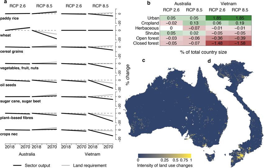
www.nature.com/scientificreports/
Commodity demand: CGE model
Commodity sector Environmental
damage functions
change
indirect
Land use: Spatial allocation
RCP2.6
Land use maps GCM
predictions
RCP8.5
Habitat Biophyscial GCM
suitability suitability predictions
direct
Suitable ranges: SDM
Figure 1. Overview of the modelling framework to capture interactions between direct and indirect drivers of
biodiversity change under climate change scenarios. We included two Representative Concentration Pathways
RCP2.6 and RCP8.5 to characterize the plausible extremes of climate change. Dark green arrows represent the
indirect pathway of climate change impacts on suitable ranges. Light green arrows indicate the direct pathway of
climate change impacts on ecological suitability. Icons from thenounproject.com.
change impacts on the distribution and extent of suitable ranges for avian species in Vietnam and Australia
(Fig. 1).
Recent advances in computable general equilibrium (CGE) m odelling18,19 bring unprecedented power to
parametrise the impacts of climate change on commodity consumption and production patterns at very high
commodity and temporal resolution across the global economy. We combine this economic modelling power
with state-of-the-art land use change modelling to spatially downscale commodity demand changes caused by
climate change4 into changes of land use patterns. In order to isolate net climate change impacts on the economy,
we parametrize only climate change damages in the CGE model, keeping all other economic parameters constant
at current baseline values. The spatial realisation of changing land use patterns varies with changes in the suit-
ability of land for particular uses and is thereby also driven by climate change7,20. Commodity demand changes
are projected annually and land use predicted in 10-year time steps, producing decadal time-series maps of land
use. Maps are integrated with climate change predictions into a biodiversity impact assessment using species
distribution models (SDMs)21–24. SDMs, fitted to current climate, land use, and other environmental variables
(Supplementary Table 1) are extrapolated to conditions in 2070 under a range of climate and land use scenarios.
Predictions of relative likelihood of occurrence are thresholded to examine changes in the ecologically suitable
ranges for 1282 bird species in Vietnam and A ustralia21–24.
Results
Direct biophysical impacts dominate changing range sizes. For birds in both regions, we forecast
major declines in ecologically suitable ranges, with severity of loss scaling with the severity of climate change
(Fig. 2). Under RCP 8.5, a much higher number of species would be expected to experience decreases of more
than half of their present ecologically suitable range compared with RCP 2.6, although variation in responses is
also greater, indicated by the much wider spread of points (Fig. 2a,b). In Australia, mean suitable range decline
under both pathways is not predicted to be as severe as in Vietnam and a smaller number of species is predicted
to lose more than half of their suitable range. For both Vietnamese and Australian birds, predicting only under
the indirect (land use change) effects of climate change results in little change to mean predicted outcomes for
species (Fig. 2a,b), though some threatened species are predicted to lose significant suitable range within their
current range due to indirect climate change impacts (see below). However, our analysis focuses on net climate
change impacts on the economy; species ranges are likely to be affected more severely when also parametrizing
other economic parameters to reflect future economic change. Mean predictions under combined direct and
indirect effects do not differ to any notable degree from those made under direct biophysical effects only. Predic-
tions under the first and third quartiles of bioclimatic variables across 15 Global Circulation Models (GCMs)
show the same trends identified in the main results (Supplementary Figure 1).
SDMs for 1436 bird species were used in the analysis of the direct and indirect impacts of climate change on
biodiversity. Discriminatory performance of the SDMs was assessed using cross-validated AUCs which varied
between 0.7 and 1.0 with a mean of 0.90 in Vietnam and 0.87 in Australia (Fig. 2c), indicating very high dis-
criminatory performance. We discarded models for 179 species with AUC < 0.7 (see “Methods” section). The
predictor variables retained in the highest fraction of models were distance to lakes (dist lakes) in Australia and
annual temperature range (bio7) in Vietnam. These are followed by dist lakes and precipitation of warmest quarter
(bio18) in Vietnam, and by minimum temperature of the coldest week (bio6) and mean diurnal temperature
Scientific Reports | (2021) 11:3304 | https://doi.org/10.1038/s41598-021-82474-z 2
Vol:.(1234567890)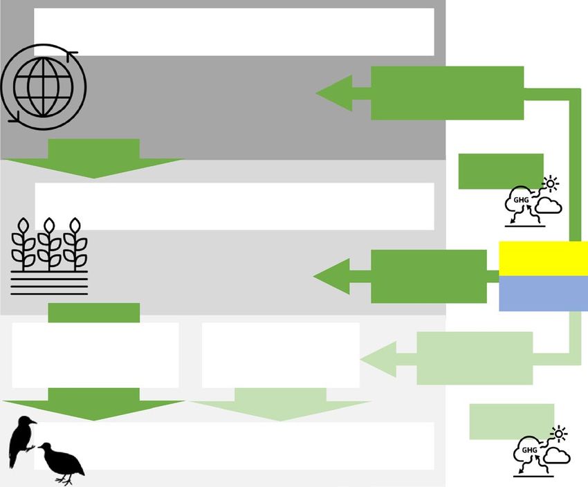
www.nature.com/scientificreports/
8x Australia Vietnam
c Australia Vietnam
a b
0.9
AUC
4x
0.7
n = 516 n = 741
d
increase
2x dila 89%
bio6 85%
bio2 78%
bio18 74%
1x bio19 72%
diri 67%
bio9 57%
1 landuse 49% Australia
decrease
x slope 36%
2
e bio7 95%
dila 89%
1 bio18 80%
x
4 bio2 77%
bio5 75%
bio19 73%
1 bio13 73%
x diri 71%
8 landuse 62% Vietnam
1 2 3 1 2 3 1 2 3 1 2 3
slope 62%
RCP 2.6 RCP 8.5 RCP 2.6 RCP 8.5
0 20 40 60 80 100
1: indirect + direct 2: indirect 3: direct Fraction of models [%]
Figure 2. Predicted changes in species’ ecologically suitable ranges. (a, b) Illustration of multiplicative changes
in species’ ecologically suitable ranges between present (2018) and 2070 for Australia and Vietnam respectively,
under three treatments (1) “indirect + direct” (combined biophysical and socio-economic impacts of climate
change), (2) “indirect” (net socio-economic impacts) and (3) “direct” (net biophysical impacts). Each point
corresponds to a species, black bars are means of ecologically suitable range changes across all species. (c) A
summary of cross-validated test Area Under the Receiver Operating Characteristics Curve values (AUCs)25 of
models in the two regions as well as the respective number of models (n) retained (AUC > 0.7)26. AUC provides
a measure of a model’s discriminatory performance in terms of how well test predictions discriminate between
occupied and unoccupied locations25,26. (d,e) Fractions of models in which a predictor was used. Full names and
definitions of all predictors can be found in Supplementary Table 1. Figure created in R version 3.5.127 (https://
www.R-project.org/).
range (bio2) in Australia. In Australia, land use was retained in about half the models. The very minor indirect
(via land use) impact predictions arise because the changes in commodity demand predicted by the CGE model
did not result in significant changes to land use in both regions (see below).
Land use changes in response to climate change vary by region. The total output of most agricul-
tural crop sectors in both regions was predicted to decrease more with increasing climate change. In particular,
in Vietnam, sectors such as oil seeds and plant-based fibres shrink by up to 20% under RCP 8.5 (Fig. 3a). The
land requirements for each sector generally increase in proportion to the overall output of each sector. This is
due to climate change impacts on crop yields as parametrised in the CGE-model: reductions in land productiv-
ity mean that more land is required to maintain sector outputs. Accordingly, in both countries, even while total
outputs tend to decrease, land requirements of agricultural sectors remain approximately the same, or increase
slightly (Fig. 3a).
The changes in land requirements for crop lead to an increase in cropland of < 0.5% of the total land area in
both regions under RCP 8.5 and a very slight decrease in Australia under RCP 2.6 (Fig. 3b). Increases in urban
land in both countries were modelled on FAOSTAT estimates of urban population growth28. In Australia, land
use changes occur locally and are concentrated in coastal areas along the north-east, south and west of the con-
tinent, although some changes also occur further inland (Fig. 3c). In Vietnam, land use change is higher overall,
with a particular concentration of change in the central-southern and northern coastal areas of the country, that
also approximately coincide with the country’s major river deltas (Fig. 3d). Given that the distributions of most
species are constrained, aggregated, and not random, small percentage changes in land use at the national scale
still have significant impacts on some species locally (Fig. 4a,c). For example, species losing more than 10% of
their currently suitable range under indirect impacts of RCP 8.5 in Vietnam include the vulnerable chestnut-
necklaced partridge (Arborophila charltonii) and the near-threatened yellow-billed nuthatch (Sitta solangiae).
These declines are highly localised and predominantly occur in the centre-south of the country (Fig. 4c). Direct
climate change impacts are more severe: 324 and 362 species lose at least 10% of their suitable ranges under
direct impacts of RCP 2.6 and RCP 8.5 respectively, with areas particularly affected across taxa under RCP 8.5
in the northern highlands and the central eastern parts of the country (Fig. 4d). Among the species losing more
Scientific Reports | (2021) 11:3304 | https://doi.org/10.1038/s41598-021-82474-z 3
Vol.:(0123456789)www.nature.com/scientificreports/
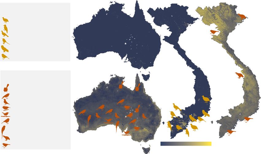
Figure 3. CGE and land use model results. (a) Future projections of commodity sector output and sector land
endowments (the area required to produce output of a sector) from CGE model under RCP 2.6 and RCP 8.5.
(b) Illustration of the percentage change of each land use in response to GTAP projections of crop sectors in (a)
and FAO urban population projections, grouped by country and RCP, relative to the whole country size. (c,d),
Intensity of predicted land use changes under indirect effects of RCP 8.5 in (c) Australia and (d) Vietnam. These
maps are derived by aggregating predicted land use changes between any two classes under the indirect impacts
of RCP 8.5 by factor 3. Figure created in R version 3.5.127 (https://www.R-project.org/).
than 95% of their current suitable range under the direct impacts of RCP 8.5 are the Chinese thrush (Turdus
mupinensis) and the critically endangered white-rumped vulture (Gyps bengalensis) (Fig. 4c,d).
In Australia, no species was found to lose more than 10% of its currently suitable range under indirect climate
change impacts, although the black-throated whipbird (Psophodes nigrogularis) loses more than 5%. A higher
number of species are affected by the direct impacts of climate change, with areas predicted to suffer particu-
larly high suitable range declines along the southern and eastern coasts, the southwest and the southeast of the
continent. In Australia, 188 and 230 species are expected to lose more than 10% of their suitable range under
RCP 2.5 and RCP 8.5 respectively.
Amongst the Australian species losing more than 95% of their suitable range under the direct impacts of
RCP 8.5 are the kalkadoon grasswren (Amytornis ballarae) and the Australasian pitpit (Anthus Australis) and a
number of other species now categorised as of least concern (Fig. 4b). This highlights the potential dangers of
climate change to species that we do not yet consider under threat, but for which extinction debts are a ccruing30.
The expected direct impacts of climate change impacts on many taxa are well researched and documented (i.e.
increased extinction risks across taxa with accelerated climate change31, northward shifts of bird distributions in
Great Britain under climate c hange32 and responses of bird abundance to climate change in the United States and
Europe33). Our findings largely agree with these trends. In both Australia and Vietnam, climate change is likely
to have extensive detrimental impacts on the climatically suitable ranges of birds. For many species, suitable
ranges decline with increasing severity of climate change (Fig. 2) and under RCP 8.5, 24% of species analysed
(in Vietnam) show likely declines in suitable ranges of greater than 50%, increasing their extinction risk in the
country severely. Our analysis shows that subject to the assumptions of this work, the relative contribution of
direct, biophysical impacts of climate change on biophysical suitability in our study area outweighs the contribu-
tion of indirect socio-economic impacts on habitat suitability via global commodity markets and resulting land
use change, also taking into account the fact that climate change impacts on the suitability of land for particular
uses. In Vietnam and Australia, bird species appear to be more severely impacted by the direct influence of
changing climates than by its indirect impacts via commodity demand and land use.
Scientific Reports | (2021) 11:3304 | https://doi.org/10.1038/s41598-021-82474-z 4
Vol:.(1234567890)www.nature.com/scientificreports/
a c d
> 10 % range decline under
indirect impacts (RCP 8.5)
Arborophila charltonii VU
Arachnothera
LC
hypogrammicum
Carpococcyx renauldi VU
Leptocoma sperata LC
Ketupa zeylonensis LC
Sitta solangiae NT
> 95% range decline under b
direct impacts (RCP 8.5)
Amytornis ballarae LC
Anthus Australis LC
Cinclosoma castanotum LC
Climacteris affinis LC
Lichenostomus ornatus LC
Pachycephala inornata LC
Parvipsitta LC
porphyrocephala
Gyps bengalensis CR
Turdus mupinensis LC
0 0.25 0.5 0.75 1
Proportion of modelled species with range declines
Figure 4. Mapping of range declines under RCP 8.5. (a–d), The proportion of avian species predicted to lose
ecologically suitable range across Australia (a,b) and Vietnam (c,d) under the indirect (a,c) and direct (b,d)
climate change impacts under RCP 8.5. Cell shading indicates the proportion of species predicted to lose
suitable range in each cell. This identifies areas of declines in species’ suitable ranges from either indirect or
direct impacts. The icons indicate locations of suitable range declines for severely affected species that lose
more than 10% (indirect) and more than 95% (direct) of their suitable ranges overall. IUCN conservation
status is given alongside taxonomic names (LC—least concern; VU—vulnerable; NT—near threatened; EN—
endangered; CR—critically endangered)29. Icon credit—http://phylopic.org. Maps created in R version 3.5.127
(https://www.R-project.org/).
Discussion
Better understanding of climate change impacts on commodity demand and supply, and how those changes
impact biodiversity should remain a research priority.
We predict economic change under two climate change scenarios, keeping all other aspects of the global
economy at current baseline values. This way, we capture and isolate the effect of climate change on the economy.
However, this approach omits other socio-economic processes that could affect supply and demand, such as
population growth, changes to economic growth, energy efficiency, and shifts in social demands. These other
factors may impact habitat and biodiversity through agricultural expansion, deforestation or urbanisation. While
this study was designed to assess the net effects of direct and indirect climate change impacts on species as a first
case study introducing our integrated assessment framework, these factors will be incorporated in future itera-
tions that include an even more comprehensive CGE parametrization (i.e. full CGE baseline scenarios with socio-
economic pathway narratives34 and integration of climate models in CGE analysis) and through improvements
to current CGE methods by including, for example, stochastic effects of natural disasters in the CGE modelling.
Our results are valid for avian taxa in Australia and Vietnam under a number of assumptions about how com-
modity demand and supply, land use and biodiversity interact to deliver outcomes predicted by our integrated
model. In our assessment framework, we follow a top-down modelling approach; within the architecture of our
CGE model, climate change affects global demand and supply of many land-based commodities, requiring sector
outputs as well as requirements of land to each sector to increase or decrease. However, mapped land use changes
corresponding to changes in land endowments to different commodity sectors do not feed back into the CGE
model. The inclusion of such feedbacks would increase the realism of both CGE and land use predictions, but
detailed knowledge of local production systems and commodity markets are required to accurately parametrise
such a model, and such models are computationally expensive35.
We chose not to produce SDMs for species with less than 20 occurrence records, to avoid the inflation of
AUC for range-restricted species and species with very low prevalence36 and to assure sufficient discrimination
between presences and background points37,38. Rare or spatially restricted species can be more vulnerable to
localised impacts such as habitat loss39, but these effects are difficult to capture when biodiversity data are poor.
We assumed unlimited dispersal ability in Vietnam and dispersal ability constrained to bioregions adjacent to
Scientific Reports | (2021) 11:3304 | https://doi.org/10.1038/s41598-021-82474-z 5
Vol.:(0123456789)www.nature.com/scientificreports/
those containing observation records in Australia. Disconnected patches of potential habitat outside of observed
ranges (but within adjacent bioregions in Australia) were counted in future predictions, regardless of whether
those areas were functionally linked (by suitable or traversable habitats) to the observed range and thus within
the dispersal range of species. This may lead to an over-estimation of habitat utilisation and a commensurate
underestimation of both direct and indirect impacts of climate change, particularly for taxa with a low dispersal
ability that rely on small pockets of habitat within their range and are unable to reach disconnected patches of
potential habitat. The importance of connectivity as a key component of habitat structure is well k nown40 and
crucial for population viability in many species with low dispersal a bility41,42. The parametrization of species’
dispersal ability and explicit modelling of landscape structure in response to land use change would allow for the
inclusion of these fragmentation effects. This may be particularly important when our framework is extended
to non-avian species.
While we found that total agricultural sector outputs decrease in both Vietnam and Australia, decreases
in land productivity mean that land use in production for some agricultural commodities were predicted to
increase slightly. We assumed a global economic equilibrium in which commodities can be substituted through
trade between regions, thus implying that global demand for land-based commodities is serviced by regions that
benefit from a comparative advantage under climate change. Where comparative advantage is due to increases
in land productivity (land use efficiency), additional land may not be required to increase outputs. However,
where this advantage is due to other economic mechanisms and not driven by the cost of converting additional
land for production, more land may be allocated to agricultural or other commodity production, increasing
habitat loss. For example, in Canada, our CGE model predicted an increase of wheat sector output by over 37%
under RCP 8.5, while land endowments increase by only 14% due to increases in land use efficiency. In India,
wheat output is estimated to increase by 8% under RCP 8.5, while land endowments to the wheat sector increase
by 6%, suggesting much lower land use efficiency in India than in Canada (see Supplementary Figure 2 for a
global, country-wise mapping of projected changes in sector outputs and land endowments of the wheat sector).
Despite lower land use efficiency, wheat production in India still grows, because growth is economically feasible
as long as it is not limited by factors arising from the sector’s context in domestic and international markets. In
both countries, increases in land use lead to agricultural expansion, but in Canada more wheat can be produced
per unit land and areas lost to wheat farming are likely to be much smaller per produced unit than in India.
Nonetheless, if wheat production occurs in parts of Canada that were previously in, for example, natural prairie,
then significant biodiversity losses may occur. Our framework provides in-depth insight into the links between
sectors and regions and allows for a better understanding of global shifts in land requirements, enabling the
fine-scale identification of hotspots for production, agricultural expansion and ultimately habitat destruction
under consideration of the global economic processes.
In this first implementation of our framework we could capture and quantify principal relationships between
climate change, the global economy, land use and avian habitat. Future uses of our approach could include
regional and global biodiversity assessments following individual policy shocks, such as the introduction or
abolishment of taxes or international trade deals, or could seek to capitalize on existing narratives of socio-
economic futures and climate change pathways (so-called Shared Socio-economic Pathways)34 to parametrise
climate adaptation policies, sustainable development goals and other aspects of socio-political transitions within
the CGE modelling. Expanding consideration of biodiversity to include non-avian taxa and explicitly dealing with
the role of connectivity and dispersal will enable a more comprehensive assessment of biodiversity impacts under
socio-economic change. A key feature of our approach is that it provides opportunity to downscale country-level
commodity demands to spatial explicit land use changes and biodiversity impacts, enabling a more meaningful
analysis of the habitat and biodiversity implications of economic shocks or the implications of trade than have
previously been possible.
Better integration of models and scenarios of biodiversity is required to guide evidence-based climate adapta-
tion strategies and to chart progress toward sustainable development goals43. Our approach to integrating eco-
nomic, land use and biodiversity values into a single model capable of high resolution, spatially-explicit predic-
tions of land use and biodiversity outcomes provides information in a form that can be used directly by planners
and managers. While spatial predictions of biodiversity and land use change have been available for decades,
being able to place these predictions coherently in a global economic context is a new and exciting development
that will bring a new level of relevance and realism to predictions in the eyes of policy and decision makers.
Methods
Study area. We focussed our analysis on Vietnam and Australia because the countries provide unique
socio-economic contexts, while hosting a similar number of bird species that are vulnerable, endangered or
critically endangered44,45. SDMs for Vietnam were built using data from a 30° × 30° tile that comprises large
parts of Southeast Asia. This enabled us to capture the occurrence of bird species present in Vietnam on larger
environmental gradients.
Climate change. We chose Representative Concentration Pathways RCP2.6 and RCP8.546 to include two
extremes of the expected radiative forcing levels. For each pathway, we acquired the 2070 predictions of 19 bio-
climatic variables47 from 15 GCM of Coupled Model Intercomparison Phase 5 (CMIP5)48. To capture variation
between GCM predictions, we determined the cell-wise first, second and third quartiles each of the 19 variables
across the 15 GCM (Supplementary Table 2).
Main results were derived by predicting land use and species distributions under the medians of these vari-
ables. We predicted both land use and species distributions under the first and third quartiles to approximate
Scientific Reports | (2021) 11:3304 | https://doi.org/10.1038/s41598-021-82474-z 6
Vol:.(1234567890)www.nature.com/scientificreports/
the range of outcomes for species across all 15 GCM (Supplementary Figure 1). In CGE models, we included
the parametrization of both climate change pathways proposed by Roson & Satori4.
CGE models. We developed an inter-temporal Global Trade and Analysis Project (GTAP) m
odel49 to sim-
ulate changes in production under different climate change scenarios. CGE models use input–output-tables
derived from national economic census data. These tables represent the inputs required in each economic sec-
tor to produce outputs and meet household and government demands (both nationally and internationally),
which in turn are affected by prices and thus supply. Sectors are linked within each national economy, but also
between economies. Producers in each country can produce various commodities to sell to domestic or foreign
households and governments. Households and governments generate their income from selling (to producers)
productive input factors (land, capital, labour, etc.) and through taxes. In our version of GTAP, the total land area
(land endowment) from which allocations are made to crop sectors (land requirements) can be changed in the
baseline. Therefore, land supply is not necessarily fixed, as is the case in most other GTAP models.
Estimations within GTAP are carried out relative to this baseline supply and we convert relative changes in
agricultural land requirements to absolute changes in cropland by using their respective shares in the total har-
vested area for a by-sector-weighting of the average relative change of all classes (Supplementary Table 3). This
weighted average change is applied on the current area under cropland to derive a future value. Accordingly, there
is a direct proportional link between changes in land requirements and changes in the total area of agricultural
land and the total area under agricultural land can change at the expense, or to the benefit, of other classes.
Since our GTAP model is a general equilibrium model, any shock to productivity will affect both the demand
and supply of an agricultural commodity. The marginal cost of production generally increases (with the loss
of productivity). At the same time, the income of households in the model will also be affected by the change
in productivity as incomes are derived from selling (or renting) productive factors (land, capital, labour, and
natural resources). As a result, prices change to equalize demand and supply and a substitution effect between
agricultural commodities and between agricultural and other commodities takes place. As a result, demand does
not stay constant. The contraction or expansion of the production of a particular crop is a result of interaction
between demand and supply for that crop (both domestically and internationally).
Our inter-temporal GTAP model uses the GTAP 9 d atabase50, which is subdivided into 139 regions and 57
commodity sectors50 and extends the GTAP model by replacing the recursive dynamic module of the current
GTAP model with a forward-looking dynamic (or inter-temporal) module, where the producer can optimise
profits overtime51,52. The inter-temporal GTAP model allows optimal investment behaviours, in which producers
in each country can adjust their decisions based on the impacts from both past and foreseeable future events.
Agents in the model can react to future threats long before their full r ealisation52. This makes the model a perfect
tool for the simulation of future phenomena like climate change.
Following Roson & Satori4, climate change impacts in our GTAP model are realised as shocks to land supply
and agricultural and labour productivity. The reduction in endowments of productive land and productivity
negatively affect the production of commodities. Agricultural commodities are expected to be the most affected.
With production shrinking more in some commodities than others, the price will adjust to balance the demand
and supply of commodities. As a result, there is a substitution effect between domestically produced products
and their competitive imports along with a substitution effect in factors of production (such as land), balancing
demands between sectors.
Unlike the Kompas et al.52 approach, which relied on a one-step simulation approach, here we apply a multi-
step simulation approach allowing the shocks to be applied into smaller successive intervals combined with
extrapolation techniques to further enhance the simulation accuracy (see Horridge et al.53 and P earson54 for
details on multi-steps CGE solution methods). The solution of the inter-temporal GTAP model in this paper
has been carried out within a parallel computing p latform19,55 with the use of PETSC56–58 and H SL59 libraries.
Land use models. We reclassified a global land use map to 8 land use classes (urban, cropland, herbaceous
ground vegetation, shrubland, open canopy forest, closed canopy forest and wetlands and barren land) (Sup-
plementary Table 1 for full list of data sources). Changes in urban land were estimated using estimates of urban
population changes60 and adjusting the amount of land under this class, assuming that urban population den-
sity remains steady through time. Future applications of this work will establish links between land use classes
related to forestry and livestock-raising, as has been demonstrated recently17.
We predicted land use maps under both pathways in 10-year time steps, using an R implementation (R pack-
age ‘lulcc’61) of the Conversion of Land Use and its Effects at Small regional extents (CLUE-S) model by Verburg
et al.62. First, we determined the local suitability for different land uses through logistic regression of land use
against the linear combination of a range of biophysical and socio-economic drivers in Generalised Linear Models
(GLMs), from 15,000 randomly sampled pixels in each region (Supplementary Table 1 for a detailed list of data,
Supplementary Figure 3 for effect sizes of predictors in each GLM). The selection of variables for land use suit-
ability models was based on work by Verburg et al.63). Correlation analysis eliminated highly correlated predictor
pairs (Spearmen’s rank correlation coefficient ≥ 0.7), always keeping the predictor whose highest correlation
with any other remaining predictor was smaller, to maximise independent information retained in the final set.
The final predictor sets were checked against literature64,65. We discarded a small number of predictors using
cross-validated Lasso penalisation in the ‘glmnet’ R-package66 and used the reduced predictor sets to build GLM
and predict to future timesteps by interpolating GCM-predicted WorldClim variables (Supplementary Table 2
for used GCM). GLM predictions produced maps of the landscape’s potential suitability for each land use class.
Transitions between classes were constrained through a matrix detailing possible transitions (Supplementary
Scientific Reports | (2021) 11:3304 | https://doi.org/10.1038/s41598-021-82474-z 7
Vol.:(0123456789)www.nature.com/scientificreports/
Table 4). We specified conversion elasticities of each class (total possible turn-over within each class) based on
literature61,62.
Projected demand changes were allocated iteratively until estimated land area demands were met20. Competi-
tion between land uses is handled in CLUE-S by allocating the land use with the highest predicted suitability in
a given cell, accounting for conversion elasticity and allowed transitions. We masked category I and II protected
areas7, precluding these areas from land use changes. Since there was no CGE-modelled future demand for her-
baceous ground vegetation and shrubland, as well as the forest classes, the overall amount of area allocated to
those land uses was what was not allocated to satisfy projected agricultural and urban demands. The proportional
allocation between each of these residual classes was determined based on their mean predicted suitability in
the landscape.
Species distribution models. Correlative species distribution models (SDM) can predict responses of
species to changing environmental conditions by extrapolating from the covariate space in which they were
observed21–24. The MaxEnt software package67 (ver. 3.3.3 k) was used to fit SDMs for 656 bird species in Australia
and 739 bird species in Vietnam, using presence-only data from the Global Biodiversity Information Facility
(GBIF)68. We filtered records to retain observations from 1950 to 2018 with more than or equal to 20 occurrence
points. We included a range of biophysical, topographic and socio-economic predictors as well as land use (Sup-
plementary Table 1). Correlation analysis eliminated highly correlated predictors (see above). Literature review
ensured that final predictor sets were ecologically meaningful to avian species across taxa32,69–71 at our aspired
scale. We kept 9 predictors for Australia and 10 predictors for Vietnam, including 5 and 6 climate predictors
respectively.
Sampling bias is a pervasive issue particularly affecting presence-only data that is often sampled opportunisti-
cally. We estimated sampling effort in response to demographic and topographic p redictors72 (Supplementary
Table 1). By selecting background points proportional to sampling effort, the its effect on the location of presence
records is largely eliminated as a form of b ias73.
Predictions were made using the estimated quartiles and medians of bioclimatic variables and the accord-
ing land use maps that were also predicted under quartiles and medians. We controlled overfitting by dropping
predictors with a permutation importance < 1%. Test AUC were estimated via fivefold cross-validation of each
model and final models built on all available records. Species for which only uninformative models were fitted
(AUC < 0.7) were excluded26.
We recorded the log ratio of the respective number of cells with relative likelihoods predicted above MaxEnt’s
MaxSSS threshold74 (where the sum of model sensitivity and specificity is maximised) between the present (2018)
and the future time step (2070) as a measure of change. In Australia, we constrained this change estimation for
each species to bioregions containing records of the species, and adjacent bioregions75.
Software and data. All data preparation and modelling for land use and SDMs was conducted in R (ver-
sion 3.5.1)27, using packages ‘lulcc’61 for land use simulations and ‘dismo’76 for MaxEnt67 models. All analyses and
spatial predictions of the land use model and SDM were performed at 0.5 arc-minute resolution; approximately
1 km at the equator. SDM building and predictions were computationally expensive and required up to 50 GB of
working memory on 12 parallel cores.
Data availability
Sources for data used in land use and species distribution modelling are listed in Supplementary Information.
Direct download links to these data sets are available in the code repository accompanying this study (see
below). We provide outputs of the CGE, land-use and species distribution models in a data repository (https://
doi.org/10.26188/5ce25391e5b60). The GTAP database that underpins GGE modelling is available from GTAP
under license. A link to a repository with the CGE modelling code that contains details of parameters settings
for global economic models and detailed commodity demand output tables for each of the scenarios modelled
is published with the code repository accompanying this study. All R-code for land use and species distribution
modelling is available online (https://doi.org/10.5281/zenodo.4461105).
Received: 14 February 2020; Accepted: 18 January 2021
References
1. Díaz, S. et al. (eds) IPBES: Summary for Policymakers of the Global Assessment Report on Biodiversity and Ecosystem Services of the
Intergovernmental Science-Policy Platform on Biodiversity and Ecosystem Services (IPBES secretariat, Bonn, 2019).
2. Struebig, M. J. et al. Targeted conservation to safeguard a biodiversity hotspot from climate and land-cover change. Curr. Biol. 25,
372–378 (2015).
3. McMichael, A. J., Woodruff, R. E. & Hales, S. Climate change and human health: present and future risks. Lancet 367, 859–869
(2006).
4. Roson, R. & Sartori, M. Estimation of climate change damage functions for 140 regions in the GTAP 9 database. J. Glob. Econ.
Anal. 1, 78–115 (2016).
5. Tol, R. S. J. Who Benefits and Who Loses from Climate Change? In Handbook of Climate Change Mitigation and Adaptation (eds
Chen, W.-Y. et al.) 1–12 (Springer, New York, 2014).
6. Veldkamp, A. & Fresco, L. O. CLUE: a conceptual model to study the conversion of land use and its effects. Ecol. Model. 85, 253–270
(1996).
7. Verburg, P. H. & Overmars, K. P. Combining top-down and bottom-up dynamics in land use modeling: exploring the future of
abandoned farmlands in Europe with the Dyna-CLUE model. Landsc. Ecol. 24, 1167–1181 (2009).
Scientific Reports | (2021) 11:3304 | https://doi.org/10.1038/s41598-021-82474-z 8
Vol:.(1234567890)www.nature.com/scientificreports/
8. Mantyka-pringle, C. S. et al. Climate change modifies risk of global biodiversity loss due to land-cover change. Biol. Conserv. 187,
103–111 (2015).
9. Oliver, T. H. & Morecroft, M. D. Interactions between climate change and land use change on biodiversity: attribution problems,
risks, and opportunities. Wiley Interdiscip. Rev. Clim. Change 5, 317–335 (2014).
10. Newbold, T. et al. Climate and land-use change homogenise terrestrial biodiversity, with consequences for ecosystem functioning
and human well-being. Emerg. Top. Life Sci. 3, 207–219 (2019).
11. Brodie, J. F. Synergistic effects of climate change and agricultural land use on mammals. Front. Ecol. Environ. 14, 20–26 (2016).
12. Brambilla, M., Pedrini, P., Rolando, A. & Chamberlain, D. E. Climate change will increase the potential conflict between skiing
and high-elevation bird species in the Alps. J. Biogeogr. 43, 2299–2309 (2016).
13. Ferrier, S. et al. (eds) IPBES. Summary for Policymakers of the Methodological Assessment of Scenarios and Models of Biodiversity
and Ecosystem Services of the Intergovernmental Science-Policy Platform on Biodiversity and Ecosystem Services (IPBES secretariat,
Bonn, 2016).
14. Leclere, D. et al. Bending the curve of terrestrial biodiversity needs an integrated strategy. Nature 585, 551–556 (2020).
15. Newbold, T. Future effects of climate and land-use change on terrestrial vertebrate community diversity under different scenarios.
Proc. R. Soc. B Biol. Sci. 285, 20180792 (2018).
16. Powers, R. P. & Jetz, W. Global habitat loss and extinction risk of terrestrial vertebrates under future land-use-change scenarios.
Nat. Clim. Change 9, 323–329 (2019).
17. Marques, A. et al. Increasing impacts of land use on biodiversity and carbon sequestration driven by population and economic
growth. Nat. Ecol. Evol. 3, 628–637 (2019).
18. Ha, P. V., Kompas, T., Thi, H., Nguyen, M. & Hoang, C. Building a better trade model to determine local effects : a regional and
intertemporal GTAP model. Econ. Model. 67, 102–113 (2016).
19. Van Ha, P. & Kompas, T. Solving intertemporal CGE models in parallel using a singly bordered block diagonal ordering technique.
Econ. Model. 52, 3–12 (2016).
20. Fuchs, R., Herold, M., Verburg, P. H. & Clevers, J. G. P. W. A high-resolution and harmonized model approach for reconstructing
and analysing historic land changes in Europe. Biogeosciences 10, 1543–1559 (2013).
21. Lawson, C. R., Hodgson, J. A., Wilson, R. J. & Richards, S. A. Prevalence, thresholds and the performance of presence-absence
models. Methods Ecol. Evol. 5, 54–64 (2014).
22. Wintle, B. A., Elith, J. & Potts, J. M. Fauna habitat modelling and mapping: a review and case study in the lower hunter central
coast region of NSW. Austral. Ecol. 30, 719–738 (2005).
23. Wintle, B. A. et al. Ecological–economic optimization of biodiversity conservation under climate change. Nat. Clim. Change 1,
355–359 (2011).
24. Thomas, C. D. Climate change and extinction risk. Nature 430, 25 (2004).
25. Jiménez-Valverde, A. Insights into the area under the receiver operating characteristic curve (AUC) as a discrimination measure
in species distribution modelling. Glob. Ecol. Biogeogr. 21, 498–507 (2012).
26. Baldwin, R. Use of maximum entropy modeling in wildlife research. Entropy 11, 854–866 (2009).
27. R Development Core Team. R: A Language and Environment for Statistical Computing. Foundation for Statistical Computing. https
://www.R-project.org/ (2020). Accessed 3 September 2018.
28. Food and Agriculture Organization of the United Nations (FAO). FAOSTAT Statistics Database (2017).
29. IUCN. The IUCN Red List of Threatened Species. Version 2018-2 (2018).
30. Kuussaari, M. et al. Extinction debt: a challenge for biodiversity conservation. Trends Ecol. Evol. 24, 564–571 (2009).
31. Urban, M. C. Accelerating extinction risk from climate change. Science 348, 571–573 (2015).
32. Gillings, S., Balmer, D. E. & Fuller, R. J. Directionality of recent bird distribution shifts and climate change in Great Britain. Glob.
Change Biol. 21, 2155–2168 (2015).
33. Stephens, P. A. et al. Consistent response of bird populations to climate change on two continents. Science 352, 84–87 (2016).
34. van Vuuren, D. P. & Carter, T. R. Climate and socio-economic scenarios for climate change research and assessment: reconciling
the new with the old. Clim. Change 122, 415–429 (2014).
35. Bryan, B. A. et al. Land-use and sustainability under intersecting global change and domestic policy scenarios: trajectories for
Australia to 2050. Glob. Environ. Change 38, 130–152 (2016).
36. van Proosdij, A. S. J., Sosef, M. S. M., Wieringa, J. J. & Raes, N. Minimum required number of specimen records to develop accurate
species distribution models. Ecography 39, 542–552 (2016).
37. Hernandez, P. A., Graham, C., Master, L. L. & Albert, D. L. The effect of sample size and species characteristics on performance of
different species distribution modeling methods. Ecography 29, 773–785 (2006).
38. Wisz, M. S. et al. Effects of sample size on the performance of species distribution models. Divers. Distrib. 14, 763–773 (2008).
39. Guisan, A. et al. Using niche-based models to improve the sampling of rare species. Conserv. Biol. 20, 501–511 (2006).
40. Taylor, P. D., Fahrig, L., Henein, K. & Merriam, G. Connectivity Is a vital element of landscape structure. Oikos 68, 571 (1993).
41. Gordon, A. et al. The use of dynamic landscape metapopulation models for forest management: a case study of the red-backed
salamander. Can. J. For. Res. 42, 1091–1106 (2012).
42. Cadenhead, N. C. R., Kearney, M. R., Moore, D., Mcalpin, S. & Wintle, B. A. Climate and fire scenario uncertainty dominate the
evaluation of options for conserving the great desert skink. Conserv. Lett. 9, 181–190 (2015).
43. UN General Assembly. Transforming Our World: The 2030 Agenda for Sustainable Development. https://www.refworld.org/docid
/57b6e3e44.html (2015). Accessed 22 November 2018.
44. BirdLife International. Country profile: Vietnam. http://www.birdlife.org/datazone/country/vietnam (2018). Accessed 21 October
2018.
45. BirdLife International. Country Profile: Australia. http://www.birdli fe.org/datazo ne/countr y/austra lia (2018). Accessed 21 October
2018.
46. van Vuuren, D. P. et al. The representative concentration pathways: an overview. Clim. Change 109, 5–31 (2011).
47. Hijmans, R., Cameron, S., Parra, J., Jones, P. & Jarvis, A. WORLDCLIM—A Set of Global Climate Layers (Climate Grids), Version
1.4.
48. Taylor, K. E., Stouffer, R. J. & Meehl, G. A. An overview of CMIP5 and the experiment design. Bull. Am. Meteorol. Soc. 93, 485–498
(2012).
49. Hertel, T. Global Trade Analysis: Modeling and Applications (Center for Global Trade Analysis, Department of Agricultural Eco-
nomics, Purdue University, West Lafayette, 1997).
50. Aguiar, A., Narayanan, B. & McDougall, R. An overview of the GTAP 9 data base. J. Glob. Econ. Anal. 1, 181–208 (2016).
51. Van Ha, P., Kompas, T., Nguyen, H. T. M. & Long, C. H. Building a better trade model to determine local effects: a regional and
intertemporal GTAP model. Econ. Model. 67, 102–113 (2017).
52. Kompas, T., Pham, V. H. & Che, T. N. The effects of climate change on GDP by country and the global economic gains from
complying with the Paris climate accord. Earth’s Future 6, 1153–1173 (2018).
53. Horridge, J. M., Jerie, M., Mustakinov, D. & Schiffmann, F. GEMPACK manual, GEMPACK Software, ISBN 978-1–921654-34-3
(2018).
54. Pearson, K. R. Solving Nonlinear Economic Models Accurately Via a Linear Representation. Working paper No. IP-55. Victoria
University, Centre of Policy Studies (1991).
Scientific Reports | (2021) 11:3304 | https://doi.org/10.1038/s41598-021-82474-z 9
Vol.:(0123456789)www.nature.com/scientificreports/
55. Kompas, T. & Ha, P. V. The ‘curse of dimensionality’ resolved: the effects of climate change and trade barriers in large dimensional
modelling. Econ. Model. 80, 103–110 (2018).
56. Balay, S. et al. PETSc users manual, Technical Report ANL-95/11—Revision 3.11. (2019).
57. Balay, S. et al. PETSc Web page. http://www.mcs.anl.gov/petsc(2019). Accessed 23 September 2018.
58. Balay, S., Gropp, W. D., McInnes, L. C. & Smith, B. F. Efficient management of parallelism in object oriented numerical software
libraries. In Modern Software Tools in Scientific Computing (eds Arge, E. et al.) (Birkhaeuser Press, Boston, 1997).
59. HSL. A collection of fortran codes for large scale scientific computation. The HSL Mathematical Software Library (2013).
60. World Bank Group. Population Estimates and Projections. http://data.worldbank.org/data-catalog/population-projection-tables
(2016). Accessed 3 May 2018.
61. Moulds, S., Buytaert, W. & Mijic, A. An open and extensible framework for spatially explicit land use change modelling: the lulcc
R package. Geosci. Model Dev. 8, 3215–3229 (2015).
62. Verburg, P. H. et al. Modeling the spatial dynamics of regional land use: the CLUE-S model. Environ. Manag. 30, 391–405 (2002).
63. Verburg, P. H., Veldkamp, T. & Bouma, J. Land use change under conditions of high population pressure: the case of Java. Glob.
Environ. Change 9, 303–312 (1999).
64. Verburg, P. H., Schulp, C. J. E., Witte, N. & Veldkamp, A. Downscaling of land use change scenarios to assess the dynamics of
European landscapes. Agr. Ecosyst. Environ. 114, 39–56 (2006).
65. Verburg, P. H., De Koning, G. H. J., Kok, K., Veldkamp, A. & Bouma, J. A spatial explicit allocation procedure for modelling the
pattern of land use change based upon actual land use. Ecol. Model. 116, 45–61 (1999).
66. Friedman, J., Hastie, T. & Tibshirani, R. Regularization paths for generalized linear models via coordinate descent. J. Stat. Soft. 33,
1–22 (2010).
67. Steven J. P., Miroslav D., Robert E. S. [Internet] Maxent software for modeling species niches and distributions (Version 3.3.3k). http://
biodiversityinformatics.amnh.org/open_source/maxent/. Accessed 12 December 2018.
68. GBIF. GBIF data portal. http://www.gbif.net/ (2016). Accessed 22 May 2018.
69. Goetz, S. J., Sun, M., Zolkos, S., Hansen, A. & Dubayah, R. The relative importance of climate and vegetation properties on patterns
of North American breeding bird species richness. Environ. Res. Lett. 9, 034013 (2014).
70. Maggini, R. et al. Assessing species vulnerability to climate and land use change: the case of the Swiss breeding birds. Divers. Distrib.
20, 708–719 (2014).
71. Coxen, C. L., Frey, J. K., Carleton, S. A. & Collins, D. P. Species distribution models for a migratory bird based on citizen science
and satellite tracking data. Glob. Ecol. Conserv. 11, 298–311 (2017).
72. Stolar, J. & Nielsen, S. E. Accounting for spatially biased sampling effort in presence-only species distribution modelling. Divers.
Distrib. 21, 595–608 (2015).
73. Phillips, S. J. et al. Sample selection bias and presence-only distribution models: Implications for background and pseudo-absence
data. Ecol. Appl. 19, 181–197 (2009).
74. Liu, C., Newell, G. & White, M. On the selection of thresholds for predicting species occurrence with presence-only data. Ecol.
Evol. 6, 337–348 (2016).
75. Morán-Ordóñez, A., Lahoz-Monfort, J. J., Elith, J. & Wintle, B. A. Evaluating 318 continental-scale species distribution models
over a 60-year prediction horizon: what factors influence the reliability of predictions?. Glob. Ecol. Biogeogr. 26, 1–14 (2016).
76. Hijmans, R. J., Phillips, S., Leathwick, J. & Elith, J. Package ‘dismo’. http://cran.r-project.org/web/packages/dismo/index.html
(2011). Accessed 6 July 2017.
Acknowledgements
This work received funding under the Australian Research Council Discovery grant DP170104795. The
authors are grateful for contributions made throughout the research phase by B. Bryan, P. Lentini, H. Kujala
and J. Elith.
Author contributions
S.K. led the modelling with contributions from P.V.H., T.K., N.G., N.C., B.W. B.W., T.K. and S.K. conceptualised
the analysis framework. S.K. led the writing of the manuscript with contributions from B.W., P.B., N.C., N.G.,
P.V.H., T.K.
Competing interests
The authors declare no competing interests.
Additional information
Supplementary Information The online version contains supplementary material availlable at https://doi.
org/10.1038/s41598-021-82474-z.
Correspondence and requests for materials should be addressed to S.K.
Reprints and permissions information is available at www.nature.com/reprints.
Publisher’s note Springer Nature remains neutral with regard to jurisdictional claims in published maps and
institutional affiliations.
Open Access This article is licensed under a Creative Commons Attribution 4.0 International
License, which permits use, sharing, adaptation, distribution and reproduction in any medium or
format, as long as you give appropriate credit to the original author(s) and the source, provide a link to the
Creative Commons licence, and indicate if changes were made. The images or other third party material in this
article are included in the article’s Creative Commons licence, unless indicated otherwise in a credit line to the
material. If material is not included in the article’s Creative Commons licence and your intended use is not
permitted by statutory regulation or exceeds the permitted use, you will need to obtain permission directly from
the copyright holder. To view a copy of this licence, visit http://creativecommons.org/licenses/by/4.0/.
© The Author(s) 2021
Scientific Reports | (2021) 11:3304 | https://doi.org/10.1038/s41598-021-82474-z 10
Vol:.(1234567890)You can also read