Assessment of meteorology vs. control measures in the China fine particular matter trend from 2013 to 2019 by an environmental meteorology index ...
←
→
Page content transcription
If your browser does not render page correctly, please read the page content below
Atmos. Chem. Phys., 21, 2999–3013, 2021
https://doi.org/10.5194/acp-21-2999-2021
© Author(s) 2021. This work is distributed under
the Creative Commons Attribution 4.0 License.

Assessment of meteorology vs. control measures in the China fine
particular matter trend from 2013 to 2019 by an environmental
meteorology index
Sunling Gong1 , Hongli Liu1 , Bihui Zhang2 , Jianjun He1 , Hengde Zhang2 , Yaqiang Wang1 , Shuxiao Wang3 ,
Lei Zhang1 , and Jie Wang4
1 StateKey Laboratory of Severe Weather & Key Laboratory of Atmospheric Chemistry of CMA,
Chinese Academy of Meteorological Sciences, Beijing 100081, China
2 National Meteorological Center, Beijing 100081, China
3 School of Environment and State Key Joint Laboratory of Environment Simulation and Pollution Control,

Tsinghua University, Beijing 100084, China
4 Hangzhou YiZhang Technology Co., Ltd., Hangzhou, China

Correspondence: Sunling Gong (gongsl@cma.gov.cn) and Hongli Liu (liuhl@cma.gov.cn)

Received: 10 April 2020 – Discussion started: 15 July 2020
Revised: 26 January 2021 – Accepted: 27 January 2021 – Published: 1 March 2021

Abstract. A framework was developed to quantitatively as-        1   Introduction
sess the contribution of meteorology variations to the trend
of fine particular matter (PM2.5 ) concentrations and to sep-    Recent observation data from the Ministry of Ecology and
arate the impacts of meteorology from the control measures       Environment of China (MEE) have shown a steady improve-
in the trend, based upon the Environmental Meteorology In-       ment of air quality across the country, especially in particular
dex (EMI). The model-based EMI realistically reflects the        matter (PM) concentrations (Hou et al., 2019). According to
role of meteorology in the trend of PM2.5 and is explicitly      the 2013–2019 China Air Quality Improvement Report is-
attributed to three major factors: deposition, vertical accu-    sued by the MEE, compared to 2013, the average concen-
mulation and horizontal transports. Based on the 2013–2019       trations of particulate matter with an aerodynamic diameter
PM2.5 observation data and re-analysis meteorological data       of less than 2.5 µm (PM2.5 ) in 74 major cities of China de-
in China, the contributions of meteorology and control mea-      creased by more than 50 % in 2019. From scientific and man-
sures in nine regions of China were assessed separately by       agement point of views, a quantitative apportionment of the
the EMI-based framework. Monitoring network observations         reasons behind the trend is critical to assess the reduction
show that the PM2.5 concentrations have declined by about        strategies implemented by the government and to guide fu-
50 % on the national average and by about 35 % to 53 % for       ture air quality control policy. However, the assessment of the
various regions. It is found that the nationwide emission con-   improvements of air quality is a complicated process that in-
trol measures were the dominant factor in the declining trend    volves the quantification of changes in the emission sources,
of China PM2.5 concentrations, contributing about 47 % of        meteorological factors, and other characteristics of the PM2.5
the PM2.5 decrease from 2013 to 2019 on the national av-         pollution, which are also interacting with each other. In order
erage and 32 % to 52 % for various regions. The meteorol-        to separate the relative degree of these factors, a comprehen-
ogy has a variable and sometimes critical contribution to the    sive analysis, including observational data and model simu-
year-by-year variations of PM2.5 concentrations, 5 % on the      lation, is needed.
annual average and 10 %–20 % for the fall–winter heavy pol-         Studies have been done extensively on the impacts of
lution seasons.                                                  weather systems on air quality. Synoptic and local meteo-
                                                                 rological conditions have been recognized as influencing the
                                                                 PM concentrations at various scales (Beaver and Palazoglu,

Published by Copernicus Publications on behalf of the European Geosciences Union.
3000                                                 S. Gong et al.: Assessment of meteorology vs. control measures in China

2006; He et al., 2017a, b; Pearce et al., 2011a, b). For the at-    reality. The mechanisms behind the variation of the time se-
mospheric aerosol pollution, the dynamic effect of the down-        ries were not investigated.
draft in the “leeward slope” and “weak wind area” of the               A chemical transport model (CTM) is an ideal tool to carry
Qinghai Tibet Plateau in winter is not conducive to the diffu-      the task of assessment by taking the meteorology, emissions
sion of air pollution emissions in the urban agglomerations of      and processes into consideration altogether. Andersson et
eastern China (Xu et al., 2015, 2002). The evolution of cir-        al. (2007) used a CTM to study the meteorologically induced
culation situation is an important factor driving the change        inter-annual variability and trends in deposition of sulfur and
in haze pollution (He et al., 2018). The local circulations,        nitrogen as well as concentrations of surface ozone (O3 ), ni-
such as mountain and valley wind and urban island circu-            trogen dioxide (NO2 ) and PM and its constituents over Eu-
lation, have a significant impact on local pollutant concen-        rope during 1958–2001. It is found that the average Euro-
tration (Chen et al., 2009; Yu et al., 2016). Previous studies      pean interannual variation, due to meteorological variability,
also revealed that PM2.5 concentration is significantly corre-      ranges from 3 % for O3 , 5 % for NO2 , 9 % for PM, 6 %–9 %
lated with local meteorological elements, such as tempera-          for dry deposition, to about 20 % for wet deposition of sulfur
ture, humidity, wind speed, and boundary layer height (He et        and nitrogen. A multi-model assessment of air quality trends
al., 2017b; Bei et al., 2020; Ma et al., 2019; He et al., 2016).    with constant anthropogenic emissions was also carried out
   In the Beijing–Tianjin–Hebei (BTH) region, a correlation         in Europe (Colette et al., 2011) and found that the magnitude
analysis and principal component regression method (Zhou            of the emission-driven trend exceeds the natural variability
et al., 2014) was used to identify the major meteorolog-            for primary compounds, concluding that emission manage-
ical factors that influenced the API (Air Pollution Index)          ment strategies have had a significant impact over the past
time series in China from 2001 to 2010, indicating that air         10 years, hence supporting further emission reduction strate-
pressure, air temperature, precipitation and relative humid-        gies. Model assessments of air quality trends in various re-
ity were closely related to air quality with a series of regres-    gions and time periods (Wei et al., 2017; Li et al., 2015) in
sion formulas. Yet the analysis was assumed to be a relatively      China were also done and yielded some useful results. For
unchanged emission whose impacts were not taken into ac-            the BTH region, Li et al. (2015) used the Comprehensive
count. On a local scale, an attempt (Zhang et al., 2017) was        Air Quality Model with extensions (CAMx) plus the Partic-
made to correlate the air pollutant levels with a combination       ulate Source Apportionment Technology (PSAT) to simulate
of meteorological factors with the development of the Sta-          the contributions of emission changes in various sectors and
ble Weather Index (SWI) at the China Meteorological Ad-             changes in meteorology conditions for the PM2.5 trend from
ministration (CMA). The SWI is a composite index which              2006 to 2013. It was found that the change in source con-
includes the advection, vertical diffusion and humidity and         tribution of PM2.5 in Beijing and northern Hebei was dom-
other meteorological factors that are related to the formation      inated by the change in local emissions. However, for Tian-
of air pollutions in a specific region or city. A higher value of   jin and central and southern Hebei Province, the change in
SWI means a weaker diffusion of air pollutants. This index          meteorology conditions was as important as the change in
had some success in assessing the meteorological impacts on         emissions, illustrating the regional difference of impacts by
air pollution, especially calibrated for a specific region, i.e.,   meteorology and emissions. However, the emission changes
Beijing. However, when applied to different areas where the         in the simulations were assumed and did not reflect the real
emission patterns and meteorological features are different,        spatio-temporal variations.
this index failed to give a universal or comparable indication         There is no surprise that previous studies could not system-
of meteorological assessment of pollution levels across the         atically catch the meteorological impacts across the whole
nation.                                                             nation as the controlling meteorological factors involving
   Using the Kolmogorov–Zurbenko (KZ) wave filter                   the characteristics of plenary boundary layers (PBLs), wind
method, Bai et al. (2015) separated the API time series into        speed and turbulence, temperature and stability, radiation and
three Chinese cities into short-term, seasonal and long-term        clouds, underlying surface as well as pollutant emissions
components and then used the stepwise regression to set up          vary greatly from region to region. A single index or cor-
API baseline and short-term components separately and es-           relation cannot be applied to the entire nation. Obviously, in
tablished linear regression models for meteorological vari-         order to systematically assess the impacts of meteorology on
ables of corresponding scales. Consequently, with the long          air pollution, these factors have to be taken into considera-
term representing the change in emissions removed from the          tion in a framework and be assessed simultaneously. This pa-
time series, the meteorological contributions alone were as-        per presents a methodology to assess the individual impacts
sumed and analyzed, pointing out that unfavorable condi-            of meteorology and emission changes, based on a model-
tions often lead to an increase by 1–13 and the favorable           derived index EMI, i.e., Environmental Meteorology Index,
conditions to a decrease by 2–6 in the long-term API series,        and observational data, providing a comprehensive analysis
respectively. Though the contributions of emissions and me-         of the air quality trends in various regions of China, with
teorological variations were separated by the research, it was      mechanistic and quantitative attributions of various factors.
only done by mathematical transformations and far from the

Atmos. Chem. Phys., 21, 2999–3013, 2021                                              https://doi.org/10.5194/acp-21-2999-2021
S. Gong et al.: Assessment of meteorology vs. control measures in China 3001
31 December 2020). From 2013 to 2019, the concentrations
showed a large change in the country, where most regions
saw a declined trend in the annual concentrations. Data show
that from 2013 to 2019, the national annual averaged PM2.5
concentrations dropped about 50 % (Fig. 2), where the haze
days have been shortened by 21.2 d from the CMA monitor-
ing data (Table 1), with some regional differences. Region-
ally, by 2019, the PM2.5 reduction rate from 2013 ranged
from 35 % to 53 %. Detailed analysis will be carried out in
the Results and discussions section.
It is noted that the PM2.5 mass concentrations by the MEE
are now reported under the observation site’s actual condi-
tions of temperature and pressure from 1 September 2018,
before which the values were reported under the standard
state (STP), i.e., 273 K and 101.325 kPa. In order to main-
tain the consistency of the data series, the PM2.5 concentra-
tions used in this study have all been converted according
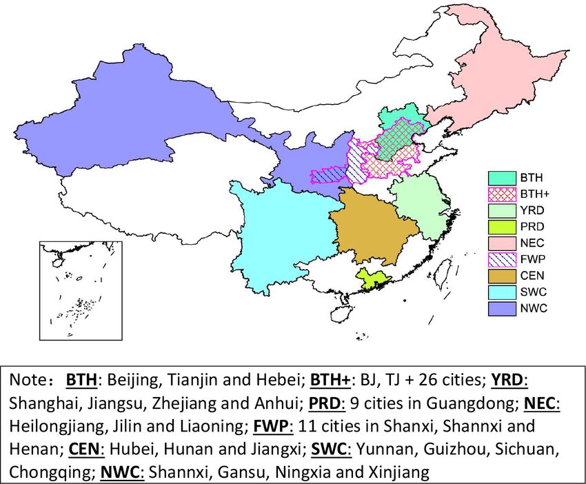
Figure 1. Analysis region separation and definition. to the new standard (MEE, 2012) (GB3095-2012) under ac-
tual conditions. Research has shown that after the change in
reporting standard, the PM2.5 concentration in most cities de-
creased, and the number of good days to meet the standard
increased (Zhang and Rao, 2019).
2.2 Meteorological data
Conventional meteorological data can provide qualitative as-
sessment of the contributions of meteorological factors to the
changes in air quality. The data used in this study are from
843 national base weather stations of the CMA from 2013 to
2019. The wind speed (WS), day with small wind (DSW),
relative humidity (RH) and haze days are used to analyze the
pollution meteorological conditions. When the daily average
wind speed is less than 2 m s−1 , a DSW is defined. Since
the haze formation is always related to stable meteorological
conditions and high aerosol mass loading, haze observation
Figure 2. National and regional trend lines of PM2.5 in China from from the CMA is also used to analyze the haze trends and the
2013 to 2019. impact of air quality on visibility. A haze day is defined with
daily averaged visibility less than 10 km and relative humid-
ity less than 85 % (Wu et al., 2014), excluding days of low
2 Methodology visibility due to precipitation, blowing snow, blowing sand,
floating dust, sandstorms and smoke.
The assessment is carried out through the combination of ob- The 2019 national annual averaged WS increased by
servational data and the EMI from model analysis. Since the 4.5 %, DSW dropped by 15.1 %, and RH decreased by 3.9 %
emission and air quality characteristics vary greatly from re- compared with 2013, with regional differences (Table 1).
gion to region in China, the analysis is divided into nine fo- Slight changes occurred when compared with 2015: WS de-
cused regions (Fig. 1). Regional air quality data (PM2.5 ) pro- creased by 0.7 %, DSW dropped by 11.3 %, and RH de-
vides the basis for the trend analysis. Separating the trend creased by 2.2 %. Overall, it can be seen that the annual haze
contribution from regional emission reduction and meteoro- days have a certain degree of correlations negatively with WS
logical variation entails a framework which is discussed be- and positively with DSW. Detailed analysis linking PM2.5
low. and meteorology will be given in the Results and discussions
section.
2.1 Particular matter (PM) observation data
The observational pollution data of PM2.5 concentrations
used in this study were from the monitoring network of
the MEE of China (http://english.mee.gov.cn/, last access:
https://doi.org/10.5194/acp-21-2999-2021 Atmos. Chem. Phys., 21, 2999–3013, 2021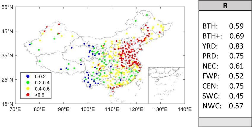
3002                                                        S. Gong et al.: Assessment of meteorology vs. control measures in China

Table 1. National and regional environmental meteorology in 2019 and comparisons with 2015 and 2013.

  Region                    Wind speed                 Days with small wind                Relative humidity               Haze (days)
                    Avg      vs. 2015    vs. 2013   Days    vs. 2015     vs. 2013     %      vs. 2015    vs. 2013   Days   vs. 2015   vs. 2013
                (m s−1 )          (%)         (%)                (%)          (%)                 (%)         (%)
  National           2.2          −0.7     +4.5     129.8     −11.3       −15.1     60.1        −2.2       −3.9     25.7     −19.0       −21.2
  BTH                2.0          −8.6     −2.2     131.0     +14.7        +9.0     56.7        −2.6       −4.2     45.2     −20.4       −26.1
  BTH+               2.0          −9.9     −1.0     114.4     +11.4        −5.6     58.3        −3.9       +0.6     54.5     −34.8       −30.3
  YRD                2.1          +2.1     −4.7     114.1     −11.2        +5.2     76.3        −0.9       +5.5     34.0     −43.8       −54.9
  FWP                1.9          +0.3    +10.9     122.8     −12.1       −25.2     59.9        −2.9       +3.3     51.6     −44.2       −43.8
  PRD                2.0          +1.9    −10.4     118.5     +16.2       +14.4     79.7        −8.0      +10.3      3.1     −10.3       −34.3
  NEC                2.7          +3.6    +12.9      55.8     −33.7       −38.4     61.6        −2.8       −5.8     13.6     −30.8       −12.4
  CEN                1.8          +3.2     +0.4     172.1      −9.4        −2.8     77.9        −1.9       +6.9     30.3     −27.9       −23.2
  SWC                1.7          +3.7    +12.2     180.7     −13.3       −16.3     74.7        −0.9       +5.7     11.1     −12.1       −12.4
  NWC                1.9          −8.4     +4.3     146.8      −2.7        −9.5     58.5         1.5       +2.8     20.2     −14.7        −6.6

Note: “+” increased; “−” decreased.

2.3    EMI – the Environmental Meteorological Index                             Mathematically, these factors are expressed as

Due to the complicated interactions of emissions, meteorol-                                    Zh
                                                                                       1                ∂C    ∂C    ∂C
ogy and atmospheric processes, a single set of meteorolog-                    iTran =                 u    +v    +w      dz,
                                                                                      hC0               ∂x    ∂y    ∂z
ical factors or a combination of them cannot quantitatively                                    0
attribute the individual factor to the changes in concentration
                                                                                               Zh

observed.                                                                              1       ∂C      ∂C      ∂C       ∂C
                                                                              iAccu =               Kx       +       Ky
   In order to quantitatively assess the impacts of meteoro-                          hC0      ∂x       ∂x     ∂y       ∂y
logical conditions on the changes in air pollution levels, an
                                                                                           0

EMI is defined as follows. For a defined atmospheric column                           ∂C      ∂C
                                                                                    +      Kz       dz,
(h) at a time t, an EMI is defined as an indication of atmo-                          ∂z      ∂z
spheric pollution level:                                                                  Zh
                                                                                       1
                             Zt                                               iEmid =        [Emis − (Vd + Ld )] dz,                         (3)
                                                                                      hC0
EMI(t) = EMI(t0) +                1EMI · dt,                       (1)                         0

                             t0                                               where the tendency is normalized by a factor C0 . For an
                                                                              application of the EMI to the PM2.5 , C0 is set to equal
where the 1EMI is the tendency that causes the changes in
                                                                              35 µg m−3 , the national standard for PM2.5 in China (MEE,
pollution level in a time interval dt defined as
                                                                              2012), and the EMI(t) is written as EMI(t)2.5 . If the EMI2.5
1EMI = iEmid + iTran + iAccu,                                      (2)        is less than 1, the concentration level will reach or be better
                                                                              than the national standard.
where the iEmid is the difference between emission and de-                       It can be seen here that these key parameters account for
position, and iTran and iAccu are the net (in minus out) ad-                  the major meteorological factors which control the air pol-
vection transports and the vertical accumulation by turbulent                 lutant levels, including wind speed and directions (u, v, w),
diffusion in the column, respectively. A positive sign of each                turbulent diffusion coefficients (Kx , Ky , Kz ) as well as dry
factor indicates a net flow of pollutants into the column, and                and wet depositions (Vd and Ld ). Therefore, under the con-
vice versa.                                                                   ditions of unchanged emissions (Emis), the EMI variation
                                                                              reflects the impacts of meteorological factors on the levels
                                                                              of atmospheric pollutants. Furthermore, because of the in-
                                                                              clusion of individual factors such as iTran, iAccu and iEmid,
                                                                              the variation of EMI(t)2.5 can be attributed to the variation
                                                                              of each factor, which gives more detailed information on the
                                                                              meteorological influence on the ambient pollutant concentra-
                                                                              tion variations. It should be pointed out that the current EMI
                                                                              has only accounted explicitly for three major physical pro-
                                                                              cesses of iTran, iAccu, and iEmid that are closely related to
                                                                              the meteorological influences. However, the secondary for-

Atmos. Chem. Phys., 21, 2999–3013, 2021                                                            https://doi.org/10.5194/acp-21-2999-2021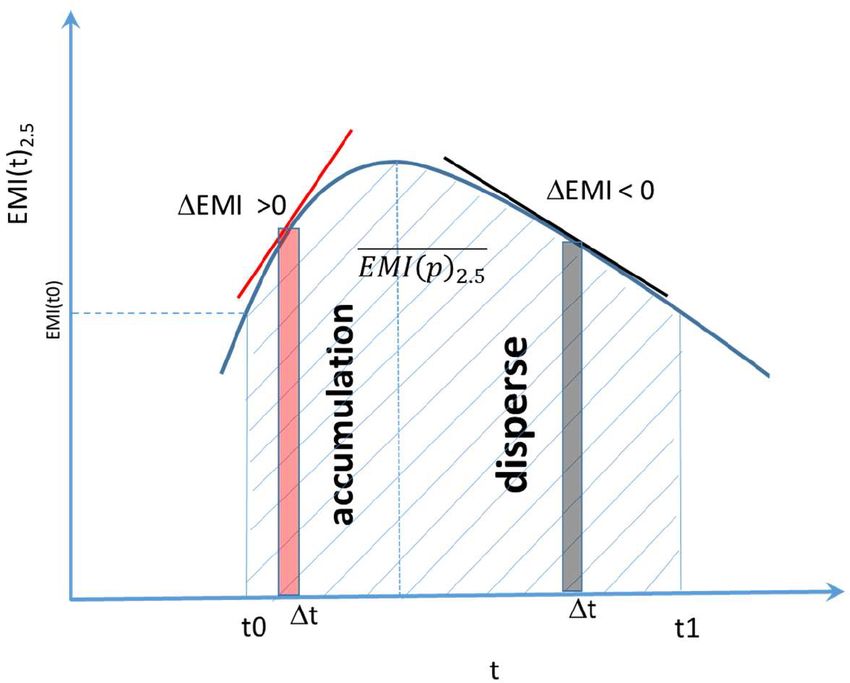
S. Gong et al.: Assessment of meteorology vs. control measures in China                                                         3003

                                                                                        1
                                                                      EMI (p)2.5 =         [EMI (0) + EMI (1) + EMI (2)
                                                                                    n+1
                                                                                 +· · · + EMI(n)]
                                                                                        1
                                                                                 =         [(n + 1)EMI (t0) + n1EMI (1) 1t
                                                                                    n+1
                                                                                 + (n − 1) 1EMI (2) 1t + (n − 2) 1EMI (3) 1t
                                                                                 + (n − 3) 1EMI (4) 1t + . . . + 1EMI(n)1t] ,
                                                                                                                                  (5)

                                                                      where n is the time steps in the period and the averaged
                                                                      EMI has been linked to the starting point EMI(0) and the
                                                                      changing rates of the EMI, i.e., 1EMI(n), at each time step.
                                                                      For monthly simulations, the initial values EMI(t0) for each
                                                                      month were set up by the averaged PM2.5 concentrations for
Figure 3. Relationship between the 1EMI, EMI(t)2.5 and                the first day from 2013 to 2019 divided by the constant C0
EMI(p)2.5 .                                                           (35 µg m−3 ).

                                                                      2.4   Assessment framework of emission controls
mation of aerosols is only implicitly considered in the EMI
as the three major physical processes are calculated from the         The EMI2.5 index provides a way to assess the meteorolog-
concentrations of aerosols (C) as indicated in Eq. (3).               ical impacts on the changes in PM2.5 concentrations at two
   For a period of time p (t0 to t1) when the averaged pollu-         time periods, i.e., January 2013 (p0) and January 2016 (p1),
tant level (e.g., PM2.5 ) is compared with EMI(t)2.5 , the time       under the assumption of unchanged emissions. However, due
integral has to be done to obtain the averaged index for the          to the national efforts of improving air quality, the year-by-
period, such as                                                       year emissions are changing rapidly and unevenly across the
                                                                      country. The changes in both emissions and meteorology are
                        Zt1
                1                                                     tangled together to yield the observed changes in ambient
EMI (p)2.5 =                  EMI(t)2.5 dt.                    (4)    concentrations. For policy makers, the emission reduction
             t1 − t0
                        t0                                            quantification is critical to guide further air quality improve-
                                                                      ments. The framework proposed here is to combine changes
The relationship among the 1EMI, EMI(t)2.5 and EMI (p)2.5             in the observed concentration levels and meteorology fac-
is illustrated in Fig. 3. It is clear that the EMI(t)2.5 is a func-   tors EMI (p)2.5 to quantify the changes caused by emission
tion of time and can be used to reflect the pollution level           changes only at two time periods.
at any time t, while the EMI (p)2.5 is the area under the                The observed concentrations at p0 and p1 are defined as
EMI(t)2.5 from times t0 to t1, which gives the averaged pol-          PM (m0, e0) and PM (m1, e1), where (m0, e0) and (m1, e1)
lution levels for the period. The derivatives of EMI(t)2.5 are        indicate the meteorology and emission status at p0 and p1,
the 1EMI, which is a positive value when the pollution is             respectively. The contribution to the observed concentration
being accumulated and a negative value when the pollution             changes between p0 and p1 by sole emission changes or
is being dispersed.                                                   control measures is defined as
   Therefore, for the period p with n discrete steps from t0
to t1, the EMI (p)2.5 represents the averaged meteorological                      PM (m0, e1) − PM(m0, e0)
                                                                      1EMIS =                              × 100 %,               (6)
influences on PM2.5 , while the sum of the positive 1EMI                                PM(m0, e0)
is the accumulation potentials and the sum of the negative
1EMI is the dispersing potentials as illustrated in Fig. 3. The       where PM (m0, e1) is a hypothetically non-measurable quan-
relationship between them is derived as follows:                      tity, indicating the PM concentration at p1 with emission e1
                                                                      and meteorology m0, which does not exist in reality. An as-
                                                                      sumption is to be made to compute this quantity using the
                                                                      EMIs. It is assumed that

                                                                      EMI(p0)2.5 /EMI(p1)2.5 = PM(m0, e1)/PM(m1, e1),             (7)

                                                                      which means that under the same emissions, the ratio of av-
                                                                      eraged EMIs under two meteorologies (m0, m1) equals the

https://doi.org/10.5194/acp-21-2999-2021                                               Atmos. Chem. Phys., 21, 2999–3013, 2021
3004                                                 S. Gong et al.: Assessment of meteorology vs. control measures in China

ratio of PM concentrations under the same two meteorolo-
gies (m0, m1). Given the nonlinear contributions of meteo-
rology and emissions to the ambient PM concentrations or
simulated EMIs, this assumption is a first-order approxima-
tion for the contributions of meteorology and emissions to
the observed concentrations. Substituting PM (m0, e1) cal-
culated from Eqs. (7) to (6) will facilitate the estimate of per-
centage contribution of emission controls to the air quality
improvement at two periods of time, independent of meteo-
rology variations.

2.5    Quantitative estimate of the EMI                             Figure 4. Correlation coefficients (R) between the EMI2.5 and the
                                                                    observed PM2.5 daily concentrations across China for 2017 and for
Finally, a process-based method is developed to calculate           typical regions averaged between 2013 and 2019.
the EMI and its components, i.e., iEmid, iTran and iAccu.
The main modeling framework used is the chemical weather
                                                                    sions on the ambient concentration changes. The EMI (p)2.5
modeling system MM5/CUACE, which is a fully coupled
                                                                    and 1EMIS form the basis for the assessment. In the Results
atmospheric model used at the CMA for national haze and
                                                                    and discussions section, the application of the platform is
air quality forecasts (Gong and Zhang, 2008; Zhou et al.,
                                                                    presented to assess the fine particular matter (PM2.5 ) changes
2012). CUACE is a unified atmospheric chemistry environ-
                                                                    in China.
ment with four major functional sub-systems: emissions, gas-
phase chemistry, aerosol microphysics and data assimilation
(Niu et al., 2008). Seven aerosol components, i.e., sea salts,      3     Results and discussions
sand/dust, EC, OC, sulfates, nitrates and ammonium salts,
are sectioned into 12 size bins with detailed microphysics of       3.1    Validation of the EMI by observations
hygroscopic growth, nucleation, coagulation, condensation,
dry depositions and wet scavenging in the aerosol module            Under the conditions of no changes in annual emissions for
(Gong et al., 2003). The gas chemistry module is based on           PM2.5 and its precursors, the daily EMI2.5 was computed
the second generation of a Regional Acid Deposition Model           by CUACE from 2013 to 2019 on a 15 × 15 km resolution
(RADM II) mechanism with 63 gaseous species through 21              across China and accompanied by its contribution compo-
photo-chemical reactions and 121 gas-phase reactions appli-         nents: iTran, iAccu and iEmid. However, in order to reflect
cable under a wide variety of environmental conditions es-          the significant changes in industrial and domestic energy
pecially for smog (Stockwell et al., 1990) and prepares the         consumptions within a year in China, a monthly emission
sulfate and SOA production rates for the aerosol module and         (Wang et al., 2011) variation was applied to the emission in-
for the aerosol equilibrium module ISORROPIA (Nenes et              ventory for computing the EMI2.5 , which more realistically
al., 1998) to calculate the nitrate and ammonium aerosols.          reflects the meteorology contributions to the PM2.5 concen-
This is the default method to treat the secondary aerosol for-      trations.
mations in CUACE. For the EMI application of CUACE,                    To evaluate the applicability of EMI2.5 , the index was
another option was also adapted to compute the secondary            compared with the observed PM2.5 concentrations. Figure 4
aerosol formations by a highly parameterized method (Zhao           shows the spatial distribution of correlation coefficients be-
et al., 2017) that computes the aerosol formation rates di-         tween PM2.5 and EMI2.5 for 2017 for all of China. The corre-
rectly from the precursor emission rates of SO2 , NO2 and           lation coefficients between EMI2.5 and PM2.5 concentrations
VOC. This option was added to facilitate timely operational         are greater than 0.4 for most of eastern China and greater
forecast requirements for the CMA. Both primary and pre-            than 0.6 for most of the assessment regions. Less satisfac-
cursor emissions of PM are based on the 2016 MEIC In-               tory correlation was found in western China, possibly due to
ventory (http://www.meicmodel.org/, last access: 31 Decem-          complex terrain and less accurate emission data over there.
ber 2020) developed by Tsinghua University for China.               Furthermore, due to the uncertainty in emissions and the dif-
   In order to quantitatively obtain each term defined in           ference in model performance for year-to-year meteorology
Eq. (3), the CUACE model was modified to extract the                simulations, the correlation coefficients may differ for differ-
change rates for the processes involved. Driven by the re-          ent years. Overall, the good correlation between them merits
analysis meteorological data, the new system CUACE/EMI              the application of EMI2.5 to quantify the meteorology impact
can be used to calculate each term in 1EMI at each time step        on PM2.5 .
(1t).                                                                  To further illustrate the applicability of EMI2.5 , the dif-
   In summary, this section presents a systematic platform to       ference of various conditions between December 2014 and
separate and assess the impacts of the meteorology and emis-        December 2015 in the BTH region was also analyzed when

Atmos. Chem. Phys., 21, 2999–3013, 2021                                               https://doi.org/10.5194/acp-21-2999-2021
S. Gong et al.: Assessment of meteorology vs. control measures in China 3005
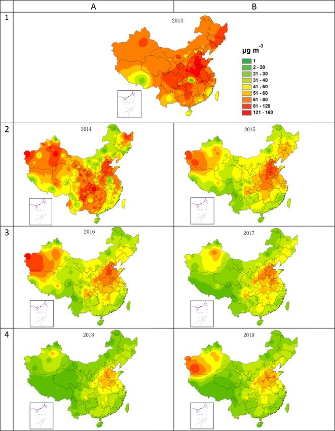
meteorological stations in the BTH region (Fig. 6a), which
indicates a large decrease in local diffusion capability. The
comparison of the wind rose map shows that the decrease
in northwesterly wind and the increase in southwesterly and
northeasterly wind occurred in December 2015 (Fig. 6b). The
change in wind fields indicates more pollutants were trans-
ported to the BTH region from Shandong, Jiangsu, Henan,
and Northeast China. These variations indirectly validate the
conclusions of adverse atmospheric transport conditions with
high iTran in December 2015.
Based on the assessment method of emission contribution
to the observed trend (Eqs. 6 and 7), the emission reduc-
tion in December 2015 as compared to 2014 was estimated
to contribute about 9.4 % (Fig. 5d) to the PM2.5 concentra-
tion decrease, compensating for the large increase caused by
meteorology, which is comparable with previous studies of
about 8.6 % reduction in emissions (Liu et al., 2017; He et
Figure 5. (a) The monthly averaged EMI2.5 and (b) monthly PM2.5
for the Decembers of 2014 and 2015 over BTH. (c) Contributions of al., 2017a) for the same 2 months. In other words, without
the sub-index to the EMI2.5 change and (d) contributions of emis- the regional emission reduction efforts, the observed PM2.5
sion and meteorology changes to PM2.5 change for the Decembers concentration in December 2015 would have had a similar
from 2014 to 2015, respectively. rate of 54.9 % increase to the worsening meteorology condi-
tions as compared with December 2014. This assessment of
emission reduction is supported by the estimate of emission
a significant change in air quality and meteorological con- inventories for the BTH region in the Decembers of 2014 and
ditions occurred. The winter of 2015 was accompanied by a 2015 by Zheng et al. (2019), who found out that the monthly
strong El Niño (ENSO) event, resulting in significant anoma- emission strengths for PM2.5 , SO2 , NOx , VOCs and NH3 in
lies for meteorological conditions in China. Analysis shows 2015 were reduced by 22.0 %, 6.9 %, 2.5 %, 2.5 % and 2.5 %,
that the meteorological conditions in December 2015 (com- respectively, as compared with 2014. The sensitivity and the
pared to December 2014) had several important anomalies, nonlinear response of PM2.5 concentrations to the air pollu-
including that the surface southeasterly winds were signif- tant emission reduction in the BTH region (Zhao et al., 2017)
icantly enhanced in the North China Plain (NCP) and the have been estimated to be about 0.43 for both primary in-
wind speeds were decreased in the middle north of eastern organic and organic PM2.5 , 0.05 for SO2 , −0.07 for NOx ,
China and slightly increased in the south of eastern China. A 0.15 for VOCs, and 0.1 for NH3 . Combining the emission
study suggests that the 2015 El Niño event had significant ef- reduction percentages between the Decembers of 2014 and
fects on air pollution in eastern China, especially in the NCP 2015 and the nonlinear response of emissions to the PM2.5
region, including the capital city of Beijing, in which aerosol concentrations results in an approximately 10.2 % ambient
pollution was significantly enhanced in the already heavily PM2.5 concentration reduction due to the emission changes.
polluted capital city of China (Chang et al., 2016). This is very close to the estimate of emission reduction con-
Figure 5 shows the monthly average EMI2.5 , PM2.5 and tribution to the December PM2.5 concentration difference of
contribution of the sub-index to total EMI2.5 in Decem- about 9.4 % between 2014 and 2015 by the EMI framework.
ber 2014 and 2015 over the BTH region. The monthly av- The applicability of the EMI to assess the meteorology
erage EMI2.5 increases by about 54.9 % from 2.1 in Decem- and emission changes is also evaluated by results from a
ber 2014 to 3.2 in December 2015, indicating worsening me- full chemical transport model (MM5/CUACE) and observa-
teorological conditions for PM2.5 pollution. The increase in tional data for PM2.5 in China for the Novembers of 2017 and
EMI2.5 is mainly contributed by adverse atmospheric trans- 2018. The averaged EMI2.5 and observational data for the 2
port conditions (Fig. 5c), which results in the increase in months were used to estimate the emission change ratio (E-
EMI2.5 reaching 3.2. With the increase in background con- Ratio in Table 2) by Eqs. (6)–(7) from 2017 to 2018. In order
centration, the deposition and vertical diffusion also increase to evaluate the correctness of this emission change estimate,
and offset the impact of adverse transport conditions to some the E-Ratio was used to adjust the emissions for Novem-
extent. ber 2018 from the base emissions of the same month for
The worsening meteorological conditions represented by 2017, which were then implemented in the MM5/CUACE to
EMI2.5 were also supported by the observations for the simulate the PM2.5 concentrations for the 2 months, respec-
two periods. The observed day with DSW, wind speed less tively. If the simulated concentration differences (M-Ratio)
than 2 m s−1 ) reveals that, except for part of southern Hebei for the 2 months were comparable with the observed con-
Province, the DSW increases by 5–15 d for 2015 in most centration differences (O-Ratio), it can be concluded that the
https://doi.org/10.5194/acp-21-2999-2021 Atmos. Chem. Phys., 21, 2999–3013, 20213006 S. Gong et al.: Assessment of meteorology vs. control measures in China
Figure 6. (a) The change in DSW (days) from December 2014 to December 2015 (December 2015–December 2014) and (b) wind rose maps
in December 2014 and December 2015 over the BTH region.
Table 2. Comparison of PM2.5 concentrations in the Novembers of 2017 and 2018 from ambient observations and from CTM simulations
by EMI-derived estimated emission changes. The emission ratio is indicated by bold font and the two concentration ratios are in bold italic
font.
City EMI2.5 Observations Emission changed CTM simulated
2017 2018 2017 2018 O-Ratio E-Ratio 2017 2018 M-Ratio
Beijing 1.8 3.6 45.7 72.8 1.59 0.80 42.3 67.5 1.59
Shanghai 2.7 2.6 42.0 40.1 0.95 1.00 52.7 51.2 0.97
Jinan 3.3 4.9 57.1 85.8 1.50 1.02 62.4 90.9 1.46
Xian 2.4 2.7 94.8 84.7 0.89 0.79 95.1 86.9 0.91
Zhengzhou 4.3 6.2 73.9 100.4 1.36 0.96 80.4 91.1 1.13
Shenyang 1.8 2.7 40.2 48.9 1.21 0.82 73.3 120.1 1.63
emission change estimated by the EMI framework was reli- FWP, CEN and NWC had the highest PM2.5 concentrations
able and could approximately represent the actual emission among the nine regions. Even though the national concen-
changes. Table 2 summarizes the analysis results of this eval- trations have been reduced significantly from 2013 by re-
uation for six typical cities. It is clear that the O-Ratios for ducing emissions, the pollution center of particular matters
the six cities are very comparable with M-Ratios, indicating has not been changed very much, located in southern Hebei
that the EMI framework can be reasonably used to estimate Province and indicating the macroeconomic structure has not
the emission changes over time. gone through a great change yet. Another phenomenon that
can be seen from the distribution is that in Northwest China,
3.2 PM2.5 trends and meteorological contributions especially in some cities of Xinjiang and Ningxia provinces,
the PM2.5 concentrations were on an increasing trend, due to
The annual averaged PM2.5 concentrations in China have certain migrating industries from developed regions in East
been decreased significantly from 2013 to 2019. Figure 7 China.
shows the observed spatial distribution of national PM2.5 Averaged for the nation, nine focused regions and Beijing,
concentrations from 2013 to 2019, respectively. These spatial the PM2.5 trend lines were shown in Fig. 2. It is seen that
distributions are consistent with those of primary and pre- all regions have had a large reduction of more than 35 %
cursor emissions of PM2.5 (Wang et al., 2011), pointing out in surface PM2.5 concentrations in 2019 as compared with
the fundamental cause of the air pollution in China. From those in 2013. The averaged national annual concentration
the spatial distributions, it is clear that the regions of BTH,
Atmos. Chem. Phys., 21, 2999–3013, 2021 https://doi.org/10.5194/acp-21-2999-2021S. Gong et al.: Assessment of meteorology vs. control measures in China 3007
Figure 7. Regional annual PM2.5 concentration distributions from 2013 to 2019.
at 36 µg m−3 has been very close to the national standard of the reduction was in the range of 45 % to 50 %, while in YRD
35 µg m−3 , while the concentrations in the PRD, SWC and and PRD the reduction was around 35 %.
NEC regions have been below the standard. Regions above As one of the key factors in controlling the ambient PM2.5
the standard are BTH+, BTH, YRD, CEN and FWP. Re- concentration variations, the annual meteorological fluctua-
gionally, the largest drop percentage of PM2.5 was seen in tions, i.e., EMI2.5 , from 2014 to 2019 with 2013 as the base
the NEC and NWC regions (Fig. 8), reaching over 50 % com- year, are shown in Fig. 9 for nine regions. Generally, the an-
pared with 2013. In the BTH, BTH+, FWP and CEN regions, nual EMI2.5 shows a positive or negative variation, reflecting
the meteorological features for that specific region. Except
https://doi.org/10.5194/acp-21-2999-2021 Atmos. Chem. Phys., 21, 2999–3013, 20213008 S. Gong et al.: Assessment of meteorology vs. control measures in China
Figure 8. Annual averaged PM2.5 concentrations in 2013 (a) and corresponding changing rates (b) from 2014 to 2019 as compared with
2013 for the nation, nine regions and Beijing.
for a couple of regions or years, most of the fluctuations are 3.3 Attribution of control measures to the PM2.5 trend
within 5 % as compared with 2013 and have no definite trend.
It can be inferred that the meteorological conditions are pos- As it is well known that the final ambient concentrations of
sibly responsible for about 5 % of the annual PM2.5 averaged any pollutants result from the emission, meteorology and at-
concentration fluctuations from 2013 to 2019 (Fig. 9b). This mospheric physical and chemical processes, separating emis-
is consistent with what has been assessed in Europe by An- sions and meteorology contributions to the pollution-level re-
dersson et al. (2007). duction entails a combined analysis of them. The analysis in
The variations in meteorological contributions (EMI2.5 ) Sect. 3.2 shows that from 2013 to 2019, the national aver-
to PM2.5 for the heavy pollution seasons of fall and winter aged PM2.5 as well as those for nine separate regions were
(1 October to 31 March) generally follow the same fluctu- all showing a gradual decline trend (Fig. 8). By 2019, 45 %–
ating pattern as the annual average but are much larger than 50 % of reductions in surface PM2.5 concentrations were
the average (Fig. 9c), over 5 % for most of the regions and achieved, while the meteorology contributions did not show
years. For specific regions and years, e.g., BTH, YRD, NEC, a definite trend as from 2013, clearly pointing out the contri-
SWC and CEN, the variations are between 10 % and 20 % bution of emission reductions in the trend. Using the analysis
as compared with 2013. Since the PM2.5 concentrations are framework for separating emissions from meteorology based
much higher in the pollution season, the larger meteorology on the monitoring data of PM2.5 and EMI2.5 (Sect. 2.4), the
variations in fall–winter would exercise more controls on the emission change contributions are estimated.
heavy pollution episodes than the annual averaged concentra- Figure 10 shows the 2013 base emissions of PM2.5 (Zhao
tions, signifying the importance of meteorology in regulating et al., 2017) and the annual changes in the emission con-
the winter pollution situations. tributions to the PM2.5 concentrations from 2014 to 2019
It is found that though most of the regions have a fluctu- as estimated from the EMI2.5 and observed PM2.5 . For the
ating EMI2.5 in the pollution season during the 2014–2019 emissions, it is found that the unit area emissions match bet-
period (Fig. 9c), the YRD and FWP show consistent favorite ter with ambient concentrations of PM2.5 in regions than
and unfavorite meteorological conditions, respectively. BTH the total emissions and the high-emission regions are BTH,
has witnessed the same unfavorite conditions as FWP, except BTH+, YRD, PRD and FWP in 2013. Nationally by 2019,
in 2017. In other words, in BTH and FWP, the decrease in the emission reduction contributions to the ambient PM2.5
ambient concentrations of PM2.5 from 2014 to 2019 has to trend ranged from 32 % to 52 % of the total PM2.5 decrease
overcome the difficulty of worsening meteorological condi- percentage, while in the BTH and BTH+ regions the re-
tions with larger control efforts. duction was more than 49 % from the 2013 base year emis-
sions, leading the national emission reduction campaign. The
emission reduction rates clearly illustrate the effectiveness
Atmos. Chem. Phys., 21, 2999–3013, 2021 https://doi.org/10.5194/acp-21-2999-2021S. Gong et al.: Assessment of meteorology vs. control measures in China 3009 Figure 9. Annual averaged EMI2.5 in 2013 (a) and corresponding changing rates for the annual average (b) and for the fall–winter seasons (c) from 2014 to 2019 as compared with 2013 in nine regions. Figure 10. Annual PM2.5 emissions (total and per unit km2 ) for 2013 (a) and corresponding changing rates (b) from 2014 to 2019 as compared with 2013 in nine regions. https://doi.org/10.5194/acp-21-2999-2021 Atmos. Chem. Phys., 21, 2999–3013, 2021
3010                                                       S. Gong et al.: Assessment of meteorology vs. control measures in China

Table 3. Observed PM2.5 difference between 2019 and 2015 as well as its attributions to meteorology and control measures for all of China,
Beijing and nine regions.

                       Regions        Observed PM2.5 difference                       Attributions
                                                                      Meteorology (EMI)         Emission controls
                                      (µg m−3 )               (%)   (µg m−3 )   Relative %    (µg m−3 )   Relative %
                       National             −10             −21.7       −4.1        −40.9        −5.9         −59.1
                       BTH                  −24             −32.4       +0.1         +0.4       −24.1        −100.4
                       BTH+                 −23             −28.8       +1.2         +5.4       −24.2        −105.4
                       YRD                  −10             −19.6       −4.0        −39.7        −6.0         −60.3
                       PRD                   −4             −12.5       +1.4        +36.0        −5.4        −136.0
                       NEC                  −14             −29.2       −4.4        −31.6        −9.6         −68.4
                       FWP                   −1              −1.8       −3.6       −362.2        +2.6        +262.2
                       CEN                  −12             −23.1       −5.5        −45.5        −6.5         −54.5
                       SWC                   −4             −12.5       −8.5       −211.5        +4.5        +111.5
                       NWC                   −6             −14.3       −5.5        −92.1        −0.5          −7.9
                       Beijing              −36             −46.2       +3.4         +9.4       −39.4        −109.4

                     Note: “+” increased; “−” decreased.

of the nationwide emission control strategies implemented                 pact by emission changes from 2015 was relevant to the in-
since 2013, and the emission reduction is the dominant fac-               terests of management to show how effective the law was.
tor for the ambient PM2.5 declining trend in China. Taking                   Table 3 summarizes the PM2.5 difference between 2019
the analysis data of PM2.5 and EMI2.5 from this study for                 and 2015 and the relative contributions of meteorology and
the BTH+ region from 2013 to 2017, it is found that the                   emission changes to the difference for all of China, Bei-
control strategy contributed more than 90 % to the PM2.5 de-              jing and nine regions. Once again, as of the end of 2019,
cline. Chen et al. (2019) estimated that the control of anthro-           the PM2.5 concentrations are all reduced from 2015, ranging
pogenic emissions contributed 80 % of the decrease in PM2.5               from −1.8 % in FWP to −46.2 % in Beijing. During this pe-
concentrations in Beijing from 2013 to 2017.                              riod of time, regions of BTH, BTH+, PRD and Beijing had
   Regionally, the emission reduction trends from 2014 to                 encountered unfavorite meteorological conditions with posi-
2019 display some unique characteristics. For the regions                 tive EMI2.5 changes, which indicated that for these regions,
of BTH, BTH+ and PRD, the year-by-year reduction rate is                  emission reductions were not only to maintain the decline
consistent, indicating that regardless of fluctuations in mete-           trend, but also to offset the unfavorite meteorological condi-
orology, these regions have had an effective emission control             tions in order to achieve the observed reductions in ambient
strategy and maintained the emission reduced year by year                 PM2.5 concentrations. By contrast, for the regions of FWP
since 2014. However, in some regions such as FWP, NEC,                    and SWC, the emission control impacts were to deteriorate
SWC and NWC, the emission reduction rates were fluctuat-                  the concentrations, implying an increase in emissions to re-
ing from 2014 to 2019, implying that the emissions in these               strain the PM2.5 concentration decrease by favorite meteoro-
regions were increased in certain years. Especially in FWP                logical conditions. For other regions, both meteorology and
from 2016 to 2017, the emissions were estimated to be in-                 emission controls contributed to PM2.5 decrease from 2015
creased by about 10 % and then decreased in 2018 and 2019,                to 2019, with the control measures contributing −7.9 % in
despite the fact that FWP experienced unfavorite meteoro-                 NWC to −68.4 % in NEC (Table 3).
logical conditions during this period.                                       Therefore, due to the diversity of meteorological condi-
   The year of 2015 is a special year in the history of China             tions and emission distributions in China, their impacts on
air pollution control. Though the systematical and network                ambient PM2.5 concentrations display unique regional char-
observations of PM2.5 started in China from 2013, it took                 acteristics. Overall, the emission controls are the dominant
about 2 years (until 2015) to evolve to the current status                factor in contributing the declining trend in China from 2013
in terms of spatial coverage and observational station num-               to 2019. However, in certain regions or certain periods of
bers, establishing a consistent and statistically comparable              years, emissions were found to be increased even with fa-
national network. In the same year, the Environmental Pro-                vorite meteorological conditions, which means the design of
tection Law of the People’s Republic of China took effect in              national control strategies has to take both meteorology and
January, signalizing the stage of lawful control of air pollu-            emission impacts simultaneously in order to achieve maxi-
tion. From the regulation assessment point of view, the im-               mum results.

Atmos. Chem. Phys., 21, 2999–3013, 2021                                                      https://doi.org/10.5194/acp-21-2999-2021
S. Gong et al.: Assessment of meteorology vs. control measures in China 3011
4 Conclusions Author contributions. SG proposed the EMI concept and led the
research project, and HL implemented the EMI concept in the mod-
eling system. BZ and HZ led the operational implementation in the
national center and provided the meteorological observational data.
YW, JH and LZ led the modeling activities and result analysis. SW
Based on a 3-D chemical transport model and its process provided the emission change data and JW provided the observa-
analysis, an Environmental Meteorological Index (EMI2.5 ) tional data of pollutants.
and an assessment framework have been developed and ap-
plied to the analysis of the PM2.5 trend in China from 2013
to 2019. Compared with observations, the EMI2.5 can real- Competing interests. The authors declare that they have no conflict
of interest.
istically reflect the contribution of meteorological factors to
the PM2.5 variations in the time series with impact mech-
anisms and can be used as an index to judge whether the
Acknowledgements. This work was supported by the National Nat-
meteorological conditions are favored or not for the PM2.5
ural Science Foundation of China (nos. 91744209, 91544232, and
pollutions in a region or time period. In conjunction with 41705080) and the Science and Technology Development Fund of
the observational trend data, the EMI2.5 -based framework the Chinese Academy of Meteorological Sciences (no. 2019Z009).
has been used to quantitatively assess the separate contribu-
tion of meteorology and emission changes to the time series
for nine regions in China. Results show that for the period Financial support. This research has been supported by the Na-
of 2013 to 2019, the PM2.5 concentrations dropped contin- tional Natural Science Foundation of China (grant nos. 91744209,
uously throughout China, by about 50 % on the national av- 91544232, and 41705080) and the Science and Technology Devel-
erage. In the regions of NWC, NEC, BTH, BEIJING, CEN, opment Fund of the Chinese Academy of Meteorological Sciences
BTH+, and SWC, the reduction was in the range of 46 % (grant no. 2019Z009).
to 53 %, while in FWP, PRD, and YRD, the reduction was
from 45 % to 35 %. It is found that the control measures of
emission reduction are the dominant factors in the PM2.5 de- Review statement. This paper was edited by Joshua Fu and re-
clining trends in various regions. By 2019, the emission re- viewed by Kun Luo and two anonymous referees.
duction contributes about 47 % of the PM2.5 decrease from
2013 to 2019 on the national average, while in the BTH re-
gion the emission reduction contributes more than 50 %, and
in the YRD, PRD, and SWC regions, the contributions were References
between 32 % and 37 %. For most of the regions, the emis-
sion reduction trend was consistent throughout the period ex- Andersson, C., Langner, J., and Bergstroumm, R.: Interannual
cept for FWP, NEC, SWC, and NWC, where the emission variation and trends in air pollution over Europe due to cli-
amounts were increased for certain years. The contribution mate variability during 1958–2001 simulated with a regional
by the meteorology to the surface PM2.5 concentrations from CTM coupled to the ERA40 reanalysis, Tellus B, 59, 77–98,
2013 to 2019 was not found to show a consistent trend, fluc- https://doi.org/10.1111/j.1600-0889.2006.00231.x, 2007.
tuating positively or negatively about 5 % on the annual aver- Bai, H.-M., Shi, H.-D., Gao, Q.-X., Li, X.-C., Di, R.-Q., and Wu,
age and 10 %–20 % for the fall–winter heavy-pollution sea- Y.-H.: Re-Ordination of Air Pollution Indices of Some Typical
sons. It is noted that the estimate of emission control contri- Cities in Beijing-Tianjin-Hebei Region Based on Meteorological
Adjustment, J. Ecol. Rural Environ., 31, 44–49, 2015.
butions was made under a first-order approximation of emis-
Beaver, S. and Palazoglu, A.: Cluster Analysis of Hourly Wind
sion and meteorology, which should be improved in the fu- Measurements to Reveal Synoptic Regimes Affecting Air Qual-
ture implementations. ity, J. Appl. Meteorol. Clim., 45, 1710–1726, 2006.
Bei, N. F., Li, X. P., Tie, X. X., Zhao, L. N., Wu, J.
R., Li, X., Liu, L., Shen, Z. X., and Li, G. H.: Im-
Code availability. This EMI system is now part of the official pact of synoptic patterns and meteorological elements on
CMA operational forecasting framework and not publicly assess- the wintertime haze in the Beijing-Tianjin-Hebei region,
able. However, for research purposes, requests for the source code China from 2013 to 2017, Sci. Total Environ., 704, 135210,
can be sent to the corresponding authors. https://doi.org/10.1016/j.scitotenv.2019.135210, 2020.
Chang, L., Xu, J., Tie, X., and Wu, J.: Impact of the 2015 El
Nino event on winter air quality in China, Sci. Rep., 6, 34275,
Data availability. The PM2.5 data are from the MEE (http:// https://doi.org/10.1038/srep34275, 2016.
english.mee.gov.cn, last access: 31 December 2020) and the meteo- Chen, Y., Zhao, C. S., Zhang, Q., Deng, Z. Z., Huang, M. Y.,
rological data are from the CMA (http://www.cma.gov.cn/en2014/, and Ma, X. C.: Aircraft study of Mountain Chimney Effect
last access: 31 December 2020). We have no authority to re- of Beijing, China, J. Geophys. Res.-Atmos., 114, D08306,
distribute the data. https://doi.org/10.1029/2008jd010610, 2009.
https://doi.org/10.5194/acp-21-2999-2021 Atmos. Chem. Phys., 21, 2999–3013, 20213012 S. Gong et al.: Assessment of meteorology vs. control measures in China
Chen, Z., Chen, D., Kwan, M.-P., Chen, B., Gao, B., Zhuang, Y., China’s Jing-Jin-Ji area, Atmos. Chem. Phys., 17, 2971–2980,
Li, R., and Xu, B.: The control of anthropogenic emissions con- https://doi.org/10.5194/acp-17-2971-2017, 2017.
tributed to 80 % of the decrease in PM2.5 concentrations in Bei- Ma, T., Duan, F. K., He, K. B., Qin, Y., Tong, D., Geng, G.
jing from 2013 to 2017, Atmos. Chem. Phys., 19, 13519–13533, N., Liu, X. Y., Li, H., Yang, S., Ye, S. Q., Xu, B. Y., Zhang,
https://doi.org/10.5194/acp-19-13519-2019, 2019. Q., and Ma, Y. L.: Air pollution characteristics and their rela-
Colette, A., Granier, C., Hodnebrog, Ø., Jakobs, H., Maurizi, tionship with emissions and meteorology in the Yangtze River
A., Nyiri, A., Bessagnet, B., D’Angiola, A., D’Isidoro, M., Delta region during 2014–2016, J. Environ. Sci., 83, 8–20,
Gauss, M., Meleux, F., Memmesheimer, M., Mieville, A., Rouïl, https://doi.org/10.1016/j.jes.2019.02.031, 2019.
L., Russo, F., Solberg, S., Stordal, F., and Tampieri, F.: Air MEE: Ambient air quality standards: GB 3095–2012, China Envi-
quality trends in Europe over the past decade: a first multi- ronmental Science Press, Beijing, China, 2012.
model assessment, Atmos. Chem. Phys., 11, 11657–11678, Nenes, A., Pandis, S. N., and Pilinis, C.: ISORROPIA: A new ther-
https://doi.org/10.5194/acp-11-11657-2011, 2011. modynamic equilibrium model for multiphase multicomponent
Gong, S. L. and Zhang, X. Y.: CUACE/Dust – an integrated inorganic aerosols, Aquat. Geochem., 4, 123–152, 1998.
system of observation and modeling systems for operational Niu, T., Gong, S. L., Zhu, G. F., Liu, H. L., Hu, X. Q., Zhou, C. H.,
dust forecasting in Asia, Atmos. Chem. Phys., 8, 2333–2340, and Wang, Y. Q.: Data assimilation of dust aerosol observations
https://doi.org/10.5194/acp-8-2333-2008, 2008. for the CUACE/dust forecasting system, Atmos. Chem. Phys., 8,
Gong, S. L., Barrie, L. A., Blanchet, J.-P., Salzen, K. V., Lohmann, 3473–3482, https://doi.org/10.5194/acp-8-3473-2008, 2008.
U., Lesins, G., Spacek, L., Zhang, L. M., Girard, E., Lin, H., Pearce, J. L., Beringer, J., Nicholls, N., Hyndman, R. J., and Tap-
Leaitch, R., Leighton, H., Chylek, P., and Huang, P.: Cana- per, N. J.: Quantifying the influence of local meteorology on
dian Aerosol Module: A size-segregated simulation of atmo- air quality using generalized additive models, Atmos. Environ.,
spheric aerosol processes for climate and air quality mod- 45, 1328–1336, https://doi.org/10.1016/j.atmosenv.2010.11.051,
els 1. Module development, J. Geophys. Res., 108, 4007, 2011a.
https://doi.org/10.1029/2001JD002002, 2003. Pearce, J. L., Beringer, J., Nicholls, N., Hyndman, R. J., Uotila,
He, J. J., Yu, Y., Xie, Y. C., Mao, H. J., Wu, L., Liu, N., and P., and Tapper, N. J.: Investigating the influence of synoptic-
Zhao, S. P.: Numerical Model-Based Artificial Neural Net- scale meteorology on air quality using self-organizing maps and
work Model and Its Application for Quantifying Impact Fac- generalized additive modelling, Atmos. Environ., 45, 128–136,
tors of Urban Air Quality, Water Air Soil Poll., 227, 235, https://doi.org/10.1016/j.atmosenv.2010.09.032, 2011b.
https://doi.org/10.1007/s11270-016-2930-z, 2016. Stockwell, W. R., Middleton, P., Change, J. S., and Tang, X.: The
He, J. J., Gong, S. L., Liu, H. L., An, X. Q., Yu, Y., Zhao, S. P., second generation Regional Acid Deposition Model Chemical
Wu, L., Song, C. B., Zhou, C. H., Wang, J., Yin, C. M., and Mechanizm for Regional Ai Quality Modeling, J. Geophy. Res.,
Yu, L. J.: Influences of Meteorological Conditions on Interannual 95, 16343–16376, 1990.
Variations of Particulate Matter Pollution during Winter in the Wang, S., Xing, J., Chatani, S., Hao, J., Klimont, Z., Cofala, J., and
Beijing-Tianjin-Hebei Area, J. Meteorol. Res., 31, 1062–1069, Amann, M.: Verification of anthropogenic emissions of China by
https://doi.org/10.1007/s13351-017-7039-9, 2017a. satellite and ground observations, Atmos. Environ., 45, 6347–
He, J. J., Gong, S. L., Yu, Y., Yu, L. J., Wu, L., Mao, H. J., Song, C. 6358, 2011.
B., Zhao, S. P., Liu, H. L., Li, X. Y., and Li, R. P.: Air pollution Wei, Y., Li, J., Wang, Z.-F., Chen, H.-S., Wu, Q.-Z., Li, J.-J., Wang,
characteristics and their relation to meteorological conditions Y.-L., and Wang, W.: Trends of surface PM2.5 over Beijing-
during 2014–2015 in major Chinese cities, Environ. Pollut., 223, Tianjin-Hebei in 2013–2015 and their causes: emission controls
484–496, https://doi.org/10.1016/j.envpol.2017.01.050, 2017b. vs. meteorological conditions, Atmos. Ocean. Sci. Lett., 10, 276–
He, J. J., Gong, S. L., Zhou, C. H., Lu, S. H., Wu, L., 283, 2017.
Chen, Y., Yu, Y., Zhao, S. P., Yu, L. J., and Yin, C. M.: Wu, D., Chen, H. Z., Meng, W. U., Liao, B. T., Wang, Y. C., Liao, X.
Analyses of winter circulation types and their impacts on N., Zhang, X. L., Quan, J. N., Liu, W. D., and Yue, G. U.: Com-
haze pollution in Beijing, Atmos. Environ., 192, 94–103, parison of three statistical methods on calculating haze days-
https://doi.org/10.1016/j.atmosenv.2018.08.060, 2018. taking areas around the capital for example, China Environ. Sci.,
Hou, X. W., Zhu, B., Kumar, K. R., and Lu, W.: Inter-annual vari- 34, 545–554, 2014.
ability in fine particulate matter pollution over China during Xu, X., Zhou, M., Chen, J., Bian, L., Zhang, G., Liu, H., Li, S.,
2013–2018: Role of meteorology, Atmos. Environ., 214, 116842, Zhang, H., Zhao, Y., Suolongduoji, and Jizhi, W.: A comprehen-
https://doi.org/10.1016/j.atmosenv.2019.116842, 2019. sive physical pattern of land-air dynamic and thermal structure
Li, X., Zhang, Q., Zhang, Y., Zheng, B., Wang, K., Chen, Y., on the Qinghai-Xizang Plateau, Sci. China Ser. D-Earth Sci., 45,
Wallington, T. J., Han, W., Shen, W., Zhang, X., and He, K.: 577–594, 2002.
Source contributions of urban PM2.5 in the Beijing-Tianjin- Xu, X. D., Wang, Y. J., Zhao, T. L., Cheng, X. H., Meng, Y. Y., and
Hebei region: Changes between 2006 and 2013 and relative im- Ding, G. A.: “Harbor” effect of large topography on haze dis-
pacts of emissions and meteorology, Atmos. Environ., 123, 229– tribution in eastern China and its climate modulation on decadal
239, 2015. variations in haze China, Chin. Sci. Bull., 60, 1132–1143, 2015.
Liu, T., Gong, S., He, J., Yu, M., Wang, Q., Li, H., Liu, W., Zhang, Yu, Y., He, J. J., Zhao, S. P., Liu, N., Chen, J. B., Mao, H. J.,
J., Li, L., Wang, X., Li, S., Lu, Y., Du, H., Wang, Y., Zhou, C., and Wu, L.: Numerical simulation of the impact of reforesta-
Liu, H., and Zhao, Q.: Attributions of meteorological and emis- tion on winter meteorology and environment in a semi-arid urban
sion factors to the 2015 winter severe haze pollution episodes in valley, Northwestern China, Sci. Total Environ., 569, 404–415,
https://doi.org/10.1016/j.scitotenv.2016.06.143, 2016.
Atmos. Chem. Phys., 21, 2999–3013, 2021 https://doi.org/10.5194/acp-21-2999-2021You can also read