Assessment of the theoretical limit in instrumental detectability of northern high-latitude methane sources using δ13CCH4 atmospheric signals ...
←
→
Page content transcription
If your browser does not render page correctly, please read the page content below
Atmos. Chem. Phys., 19, 12141–12161, 2019
https://doi.org/10.5194/acp-19-12141-2019
© Author(s) 2019. This work is distributed under
the Creative Commons Attribution 4.0 License.

Assessment of the theoretical limit in instrumental detectability
of northern high-latitude methane sources using δ 13CCH4
atmospheric signals
Thibaud Thonat1 , Marielle Saunois1 , Isabelle Pison1 , Antoine Berchet1 , Thomas Hocking1 , Brett F. Thornton2 ,
Patrick M. Crill2 , and Philippe Bousquet1
1 Laboratoiredes Sciences du Climat et de l’Environnement, LSCE/IPSL, CEA-CNRS-UVSQ, Université Paris-Saclay,
91191 Gif-sur-Yvette, France
2 Department of Geological Sciences and Bolin Centre for Climate Research, Stockholm University, Svante Arrhenius väg 8,

106 91 Stockholm, Sweden

Correspondence: Marielle Saunois (marielle.saunois@lsce.ipsl.fr)

Received: 20 November 2018 – Discussion started: 26 November 2018
Revised: 12 July 2019 – Accepted: 26 July 2019 – Published: 30 September 2019

Abstract. Recent efforts have brought together bottom-             sions requires accuracies lower than 0.05 ‰ at coastal Rus-
up quantification approaches (inventories and process-based        sian sites (even lower for other sites). Freshwater emissions
models) and top-down approaches using regional observa-            would be detectable with an uncertainty lower than 0.1 ‰ for
tions of methane atmospheric concentrations through in-            most continental sites. Except Yakutsk, Siberian sites require
verse modelling to better estimate the northern high-latitude      stringent uncertainty (lower than 0.05 ‰) to detect anthro-
methane sources. Nevertheless, for both approaches, the rel-       pogenic emissions from oil and gas or coal production. Re-
atively small number of available observations in northern         mote sites such as Zeppelin, Summit, or Alert require a daily
high-latitude regions leaves gaps in our understanding of the      uncertainty below 0.05 ‰ to detect any regional sources.
drivers and distributions of the different types of regional       These limits vary with the hypothesis on isotopic signatures
methane sources. Observations of methane isotope ratios,           assigned to the different sources.
performed with instruments that are becoming increasingly
affordable and accurate, could bring new insights on the con-
tributions of methane sources and sinks. Here, we present
the source signal that could be observed from methane iso-         1   Introduction
topic 13 CH4 measurements if high-resolution observations
were available and thus what requirements should be ful-           Atmospheric methane (CH4 ) is a potent climate forcing gas,
filled in future instrument deployments in terms of accuracy       responsible for more than 20 % of the direct additional radia-
in order to constrain different emission categories. This the-     tive forcing caused by human activities since pre-industrial
oretical study uses the regional chemistry-transport model         times (Ciais et al., 2013; Etminan et al., 2016). After stay-
CHIMERE driven by different scenarios of isotopic signa-           ing nearly constant between 1999 and 2006, methane con-
tures for each regional methane source mix. It is found that       centrations have been increasing again (Dlugokencky et al.,
if the current network of methane monitoring sites were            2011; Saunois et al., 2016). The explanations of this renewed
equipped with instruments measuring the isotopic signal con-       accumulation are still widely debated. Recent studies, how-
tinuously, only sites that are significantly influenced by emis-   ever, stress the major role played by microbial sources, par-
sion sources could differentiate regional emissions with a         ticularly in the tropics (Schaefer et al., 2016; Nisbet et al.,
reasonable level of confidence. For example, wetland emis-         2016; McNorton et al., 2016; Saunois et al., 2017), together
sions require daily accuracies lower than 0.2 ‰ for most of        with uncertain contributions of fossil-fuel-related emissions
the sites. Detecting East Siberian Arctic Shelf (ESAS) emis-       (Schwietzke et al., 2016; Saunois et al., 2016) associated

Published by Copernicus Publications on behalf of the European Geosciences Union.

12142                                      T. Thonat et al.: Methane source detectability using δ 13 CCH4 atmospheric signal

with a probable decrease in biomass burning emissions (Wor-        98.8 %, 1.1 %, and 0.06 % (Bernard, 2004). An isotopic sig-
den et al., 2017). Decreases in atmospheric sinks (Naus et         nature characterizes each source and sink. The fractionation
al., 2019; Rigby et al., 2017; Turner et al., 2017) have also      between the different isotopes is driven by source and sink
been postulated to contribute to the rise, though changes in       processes that vary in space and time (Schwietzke et al.,
methane sinks cannot explain this rise by themselves.              2016). Microbial sources produce methane depleted in heavy
   Although the northern high latitudes (> 60◦ N) represent        isotopes. The isotopic signatures of biological sources vary
only about 4 % of global methane emissions (Saunois et al.,        depending on the metabolic pathway of formation, on the
2016) and do not seem to be a main contributor to the in-          nature of the degraded organic matter, on its stage of degra-
creasing trend of the past decade (e.g. Nisbet et al., 2016), it   dation, and on temperature (Whiticar, 1999). Thermogenic
is a region of major interest in the context of climate change     sources related to fossil fuels emit methane that tends to be
and the associated risks. The Arctic is particularly sensi-        not as depleted in heavy isotopes as microbial sources. Py-
tive to climate-driven feedbacks. For instance, higher tem-        rogenic sources related to incomplete biomass combustion
peratures may favour methane production from wetlands and          are even less depleted, with combustion of C3 plants con-
methane release from thawing permafrost, as protected car-         tributing lighter signatures than C4 plants. Sink processes
bon becomes available to remineralization. This could drive        also influence methane’s isotopic composition. The isotopic
a sustained carbon feedback to climate change (Schuur et           fractionations associated with the reaction with OH and the
al., 2015). Most major source types for methane are present        uptake by soils enrich atmospheric methane in heavier iso-
in the northern high latitudes: natural wetlands, oil and gas      topes comparison to the mean source signature. Atmospheric
industry, and peat and forest burnings. There are also other       methane carries the isotopic signature resulting from the
sources that have received increasing attention over the past      summed value of all of its sources and sinks. Though mea-
decade: freshwater systems (Walter et al., 2007; Bastviken         surements of 12 CH3 D exist, only 12 CH4 and 13 CH4 are con-
et al., 2011; Tan and Zhuang, 2015; Wik et al., 2016), sub-        sidered in this study because they are the most abundant
sea permafrost and hydrates in the East Siberian Arctic Shelf      methane isotopologues in the atmosphere and as such are
(ESAS, in the Laptev and East Siberian seas; Shakhova et           easier to measure than 12 CH3 D. Regular measurements us-
al., 2010; Berchet et al., 2016; Thornton et al., 2016a), and      ing flask samples have existed since the early 2000s for
terrestrial thermokarst (Wik et al., 2016).                        δ 3 CCH4 . Unfortunately 12 CH3 D flask measurement series are
   Methane sources and sinks can be estimated by a vari-           scarce, with no published Arctic series in recent years. Laser
ety of approaches generally classified as either top-down          spectrometer-based instruments for δ 3 CCH4 continuous mea-
(driven by atmospheric transport and concentration data) or        surements are currently being, or have been, settled at differ-
bottom-up (driven by inventories and process-based models;         ent locations (e.g. Zeppelin mountain, Svalbard, since 2018),
e.g. Saunois et al., 2016). Our understanding of the methane       while this is less the case for 12 CH3 D, most likely because
global budget and its evolution is limited by the uncertain-       only one instrument is commercially available.
ties about sources (their location, intensity, seasonality, and        The isotopic variations are small: the ratio of 13 C/12 C
proper classification) and sinks, by the representative cover-     in methane is expressed in conventional delta notation as
age of the current observational surface network, by the bi-       δ 13 CCH4 , which is the part per thousand deviation of the ratio
ases of satellite-based data (e.g. Bousquet et al., 2018), and     in a sample to that in an international standard:
by the quality of atmospheric transport models (e.g. Patra et
                                                                   δ 13 CCH4 = [(Rsample /Rstandard ) − 1] × 1000 ‰,            (1)
al., 2018). In particular, the discrepancies between bottom-up
and top-down estimates remain a major concern both glob-           where R is  13 C/12 C of either the sample or of a community-
ally (Saunois et al., 2016) and in the Arctic (Thornton et al.,    determined standard (currently Vienna Pee Dee Belemnite,
2016b; Thompson et al., 2017). Methane sources are partic-         VPDB; Craig, 1957).
ularly numerous and are temporally and spatially variable,            The use of stable isotopes for discriminating methane
especially when compared to carbon dioxide (Saunois et al.,        sources is not new (Schoell, 1980). Isotope data can bring a
2016). This makes it challenging to allocate emissions to          valuable constraint on the methane budget (Mikaloff Fletcher
each particular source as illustrated in Berchet et al. (2015),    et al., 2004) and can be relevant in the elimination of some
who studied overlapping wetland and anthropogenic emis-            emission scenarios used to explain methane evolutions glob-
sions in Siberian lowlands with a top-down approach. Im-           ally (Monteil et al., 2011; Saunois et al., 2017) or region-
proving the attribution of methane emissions to specific pro-      ally, for example in the Arctic (Warwick et al., 2016). Since
cesses in top-down approaches can benefit from the addi-           2007, globally averaged atmospheric methane concentrations
tional information (on top of the total concentrations) pro-       have been steadily increasing and at the same time atmo-
vided by the ratios of stable isotopes in atmospheric methane      spheric methane has become more depleted in 13 C. Nisbet et
concentrations.                                                    al. (2016) found the post-2007 shift in the δ 13 CCH4 value of
   There are three main stable isotopologues of methane that       the global atmospheric mean concentration to be −0.17 ‰.
are commonly measured: 12 CH4 , 13 CH4 , and 12 CH3 D. Their       This shift signifies major ongoing changes in the methane
respective abundances in the atmosphere are approximately          budget and can be used to bring additional constraints on

Atmos. Chem. Phys., 19, 12141–12161, 2019                                          www.atmos-chem-phys.net/19/12141/2019/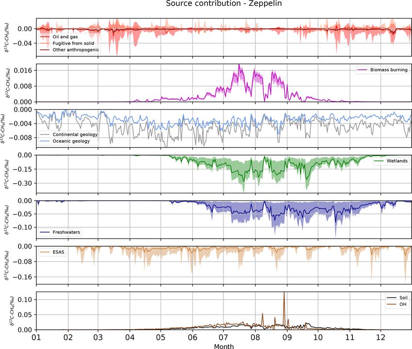
T. Thonat et al.: Methane source detectability using δ 13 CCH4 atmospheric signal                                            12143

the source partitioning (Saunois et al., 2017). Using a box        which would have been missed without the isotopic informa-
model, Schaefer et al. (2016) estimated the δ 13 CCH4 value        tion. In the Arctic, the importance of wetland emissions has
of the post-2007 globally averaged source needed to match          been highlighted with the analysis of isotopic data from air-
the observed δ 13 CCH4 evolution to be −59 ‰. They con-            craft, ships, and surface stations (Fisher et al., 2011; O’Shea
cluded that the post-2007 rise was driven by microbial emis-       et al., 2014; France et al., 2016). Field campaigns are also
sions, in particular from agricultural sources. The Schaefer et    regularly organized to measure the isotopic signatures of var-
al. (2016) estimate was used to validate the sectorial partition   ious sources (Pisso et al., 2016; McCalley et al., 2014; Fisher
of the emission changes for the period 2000–2012 retrieved         et al., 2017).
by Saunois et al. (2017). However, large uncertainties and             The paucity of isotopic measurements to constrain top-
overlaps remain for source signatures, implying that δ 13 CCH4     down atmospheric inversions is another limitation. Inver-
cannot point towards a unique solution.                            sions assimilating both total methane and isotope data are
   Three main limitations remain in the use of isotopic data       few; they use only flask sampling data and rely on a few
to improve our knowledge of methane sources and sinks: the         sites around the world. This, together with the lack of infor-
wide ranges of isotopic signatures, the lack of information        mation on isotopic signatures, can explain why such multi-
to estimate these signatures, and the lack of atmospheric iso-     constraint inversions have mostly been conducted with sim-
topic data to assimilate in top-down approaches (Tans, 1997).      ple box models so far (e.g. Schaefer et al., 2016). How-
   Isotopic signatures span large ranges of values, with typ-      ever, laser spectrometers can now provide continuous ob-
ical ranges being −70 ‰ to −55 ‰ for microbial, −55 ‰              servations of methane isotopes with satisfying performance
to −25 ‰ for thermogenic, and −25 ‰ to −13 ‰ for py-               (Santoni et al., 2012). Moreover, such high-frequency and
rogenic sources (Kirschke et al., 2013). Actually, significant     high-precision isotope measurements were shown, if applied
overlap occurs (see Thornton et al., 2016b and Sect. 2.4: e.g.     to the current observational network, to potentially reduce
−110 ‰ to −50 ‰ for microbial signatures and −80 ‰ to              uncertainties to source inversion in all sectors, even at the
−17 ‰ for coalfields). Modelling studies do not always re-         national scale (Rigby et al., 2012).
flect these ranges because they choose only one or a few val-          Even though long-term continuous atmospheric 13 CH4
ues for each source. McCalley et al. (2014) found that us-         time series are not yet available, it seems important to eval-
ing the commonly used isotopic signature for wetlands for          uate their potential to improve our knowledge on methane
future emissions related to thawing permafrost could entail        sources and sinks. A first step is the modelling of the iso-
overestimations of a few teragrams CH4 and an erroneous            topic signals to be expected at possible monitoring sites,
source apportionment. Regarding coal emissions, Zazzeri et         taking into account the range of isotopic signatures of the
al. (2016) pointed out that global models usually use a sig-       different sources. The northern high-latitude region is cho-
nature of −35 ‰ for coal, while measured values are be-            sen as a test region because of the significant potential of
tween −30 ‰ and −60 ‰ depending on the coal type and               the climate–carbon feedback mentioned earlier and because
depth (from anthracite to bituminous). Recently, Sherwood          methane emissions may overlap less (in time and space) than
et al. (2017) compiled a global comprehensive database of          in the tropics for instance.
δ 13 CCH4 and other methane isotopic signatures for fossil             Following Thonat et al. (2017), who estimated the de-
fuel, microbial, and biomass burning sources. They pointed         tectability of methane emissions at Arctic sites measuring
out that most modelling studies relied on a set of canonical       total CH4 , this paper aims at extending this approach to
isotopic signature values that circulated within the modelling     δ 13 CCH4 observations, even if they do not yet exist. After pre-
community, which could have led to the use of erroneous            senting the 24 existing monitoring sites in the northern high
values. For example, using a previous version of the Sher-         latitudes and the modelling framework (Sect. 2), we evaluate
wood database, Schwietzke et al. (2016) revised the fossil         how well our model simulates δ 13 CCH4 at the five sites where
fuel methane emissions upward by about 50 % for the past           it is already monitored (Sect. 3.1). Then, the atmospheric sig-
3 decades.                                                         nals of the various northern high-latitude methane sources at
   The lack of information on δ 13 CCH4 signatures is also         these sites are estimated (Sect. 3.2) before determining their
a limitation for identifying sources of distinctive methane        detectability based on instrumental constraints and on the un-
plumes (France et al., 2016). However, several recent              certainties of the isotopic signatures (Sect. 3.3).
measurement campaigns showed the value of determining
δ 13 CCH4 for source apportionment. For example, Röckmann
et al. (2016) have deployed high-frequency isotopic mea-           2     Measurements and modelling framework
surements of both δ 13 CCH4 and δDCH4 at Cabauw in Eu-
rope and were able to identify specific events and to allocate     2.1    Measurements
them to specific anthropogenic sources (ruminants, natural
gas, or landfills). Similarly, the isotopic analyses led by Cain   Measurements of the isotopic ratio in atmospheric methane
et al. (2016) from aircraft data in the North Sea made it pos-     for 2012 come from five northern high-latitude surface sites
sible to identify a source in a plume downwind of gas fields,      (White et al., 2018). The locations of these sites are shown in

www.atmos-chem-phys.net/19/12141/2019/                                           Atmos. Chem. Phys., 19, 12141–12161, 2019
12144                                       T. Thonat et al.: Methane source detectability using δ 13 CCH4 atmospheric signal

Table 1. Description of the 24 sites measuring methane used in this study and included in our polar domain.

                     Code     Sites              Coordinates             Altitudes (m a.s.l)   δ 13 CCH4 observations
                     ALT      Alert              82.45◦ N, 62.52◦ W                     36               Y
                     AMB      Ambarchik          69.62◦ N, 162.30◦ E                     5               –
                     BKL      Baker Lake         64.17◦ N, 95.50◦ W                     10               –
                     BRW      Barrow             71.32◦ N, 156.60◦ W                     2               Y
                     BCK      Behchokò           62.80◦ N, 116.10◦ W                   179               –
                     CBB      Cambridge Bay      69.10◦ N, 105.10◦ W                    30               –
                     CAR      CARVE Tower        65.00◦ N, 147.60◦ W                   611               –
                     CHS      Cherskii           68.61◦ N, 161.34◦ E                    23               –
                     CHL      Churchill          58.75◦ N, 94.07◦ W                      9               –
                     CBA      Cold Bay           55.21◦ N, 162.72◦ W                    25               Y
                     DEM      Demyanskoe         59.79◦ N, 70.87◦ E                     71               –
                     IGR      Igrim              63.19◦ N, 64.42◦ E                     53               –
                     INU      Inuvik             68.30◦ N, 133.50◦ E                    10               –
                     KRS      Karasevoe          58.25◦ N, 82.42◦ E                     78               –
                     NOY      Noyabrsk           63.43◦ N, 75.78◦ E                    100               –
                     PAL      Pallas             67.97◦ N, 24.12◦ E                    301               –
                     ICE      Stórhöfði          63.40◦ N, 20.29◦ W                    118               –
                     SUM      Summit             72.60◦ N, 38.42◦ W                   3178               Y
                     TER      Teriberka          69.20◦ N, 35.10◦ E                     83               –
                     TIK      Tiksi              71.59◦ N, 128.92◦ E                   123               –
                     VGN      Vaganovo           54.50◦ N, 62.32◦ E                    197               –
                     YAK      Yakutsk            62.09◦ N, 129.36◦ E                   198               –
                     ZEP      Zeppelin           78.91◦ N, 11.89◦ E                    475               Y
                     ZOT      Zotino             60.80◦ N, 89.35◦ E                    104               –

Fig. 1, and their characteristics are given in Table 1. Most of         isotope ratio being computed offline a posteriori. Following
them are considered to be sampling background air: Alert                Thonat et al. (2017), the domain has a regular kilometric res-
is located in northern Canada; Zeppelin (Ny-Ålesund) is                 olution of 35 km, which avoids numerical issues due to grid
on a mountaintop in the Svalbard archipelago; Cold Bay is               cells that are too small, close to the pole, and encountered
in the Alaska Peninsula; and Summit is at the top of the                in regular latitude–longitude grids. It covers all longitudes
Greenland Ice Sheet. The Barrow observatory (now known as               above 64◦ N but extend partially to 39◦ N, as illustrated in
Utqiaġvik), located in the North Slope of Alaska, is more af-          Fig. 1. The troposphere is divided into 29 vertical levels from
fected by local wetland emissions. The NOAA Earth System                the surface to 300 hPa (∼ 9000 m).
Research Laboratory (NOAA ESRL) is responsible for the                     CHIMERE solves the advection–diffusion equation and is
collection and analysis of the weekly flask samples. The iso-           forced using meteorological fields from the ECMWF (Eu-
topic composition is determined by INSTAAR (Institute of                ropean Centre for Medium Range Weather Forecasts, http:
Arctic and Alpine Research) of the University of Colorado.              //www.ecmwf.int/; last access: 18 September 2019) forecasts
All data are reported in conventional delta notation, in per mil        and reanalyses. Wind, temperature, water vapour, and other
(‰). The δ 13 CCH4 observations are given with a precision of           meteorological variables are given with a 3 h time resolu-
better than 0.1 ‰ (White et al., 2018). All data without re-            tion, at ∼ 0.5◦ spatial resolution, and 70 vertical levels in the
ported issues in collection or analyses are selected; outliers          troposphere. Initial and boundary concentrations of 12 CH4
above 3σ of the variability at the station are discarded.               and 13 CH4 come from a global simulation of the general cir-
   Other sites where atmospheric methane is measured are                culation model LMDZ (Hourdin et al., 2006) for the year
also included in this study. They do not provide δ 13 CCH4 ob-          2012. This global simulation used emission fluxes (including
servations, but we evaluate their potential in doing so. Their          ORCHIDEE for wetland emissions, EDGARv4.2 for anthro-
description is given in Table 1.                                        pogenic emissions other than biomass burning, and GFED4.1
                                                                        for biomass burning emissions) that were adjusted in order
2.2   Model description                                                 to obtain a reasonable agreement at the global scale between
                                                                        the simulated isotopic signal and the flask measurements of
The Eulerian chemistry-transport model CHIMERE (Vautard                 the NOAA ESRL network (Dlugokencky et al., 1994). These
et al., 2001; Menut et al., 2013) is used to simulate tropo-            global fields have a 3 h time resolution and 3.75◦ × 1.875◦
spheric 12 CH4 and 13 CH4 concentrations separately, with the           spatial resolution. These meteorological and concentration

Atmos. Chem. Phys., 19, 12141–12161, 2019                                                www.atmos-chem-phys.net/19/12141/2019/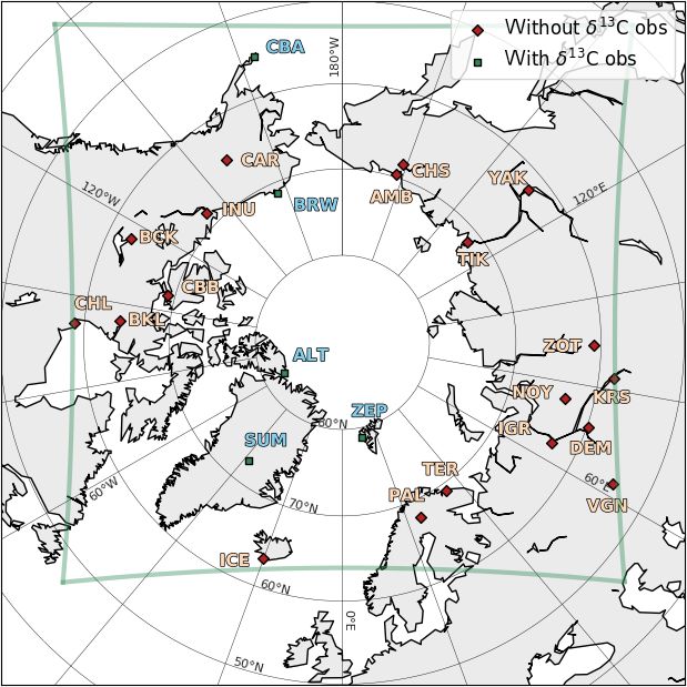
T. Thonat et al.: Methane source detectability using δ 13 CCH4 atmospheric signal                                                  12145

Figure 1. Delimitation of the studied polar domain (green line), the location of the 24 measurement sites used in this study and measuring
atmospheric methane. Five stations (blue squares) include flask measurements of δ 13 CCH4 . The station name abbreviations are given in
Table 1.

fields are interpolated in time and space within the grid of           2–4 weeks (typical mixing time of air masses in the domain
the CHIMERE domain.                                                    with the chosen model set-up spanning high northern-latitude
   The model is run with various tracers, each one corre-              regions), but this has little impact on our conclusions. No
sponding either to the 12 CH4 or to the 13 CH4 component of a          chemistry is included in the multi-tracers simulation, but an-
methane source. Simulated 12 CH4 and 13 CH4 of all sources             other simulation including the reaction with OH is carried out
are then used in the calculation of δ 13 CCH4 . This allows us         in order to assess the contribution of this major sink. More
to analyse the contribution of each source in δ 13 CCH4 . Three        details on the aforementioned emission categories are given
pairs of tracers correspond to anthropogenic sources: emis-            below in Sect. 2.3.
sions from oil and gas, emissions from solid fuels (coal),
and other anthropogenic emissions (mostly from enteric fer-            2.3   Input emission data
mentation and solid waste disposal). One pair of tracers cor-
responds to biomass burning. Two pairs correspond to geo-              Surface emissions used as inputs in the model come from var-
logical sources: continental micro- and macroseepages; and             ious inventories, models, and data-driven studies. The emis-
marine seepages. Three pairs correspond to other natural               sions used are the same as in Thonat et al. (2017), in which
sources: wetlands, freshwater systems, and emissions from              they are described and discussed in more detail; we provide
the ESAS. Another pair of tracers corresponds to soil uptake           a summary below and in Table 2.
and is considered as a negative surface source. Finally, one              All anthropogenic emissions are taken from the
pair of tracers corresponds to the boundary conditions. No             EDGARv4.2FT2010 yearly product (Olivier and Janssens-
pair of tracers is implemented for the initial conditions: sim-        Maenhout, 2012). When possible, the 2010 data are
ulations in January are partly influenced by prescribed initial        updated using FAO (Food and Agriculture Organiza-
conditions from global fields during the spin-up period of             tion, http://www.fao.org/faostat/en/\#data/, last access: 18

www.atmos-chem-phys.net/19/12141/2019/                                                Atmos. Chem. Phys., 19, 12141–12161, 2019
12146                                        T. Thonat et al.: Methane source detectability using δ 13 CCH4 atmospheric signal

Table 2. Methane emissions and isotopic signatures in the studied domain (see text within Sects. 2.3 and 2.4). Emission and sink fluxes used
here are the same as in Thonat et al. (2017).

                  Type of source or sink    Emissions (Tg CH4 yr−1 )     δ 13 CCH4 (‰)      KIE     Range δ 13 CCH4 (‰)
                  Oil and gas                                    11.9             −46                         −40, −50
                  Coal mining                                     4.7             −55                         −50, −65
                  Animals                                         1.3             −62                                –
                  Landfills                                       1.1             −52                                –
                  Total anthropogenic                            20.5                –                               –
                  Biomass burning                                 3.1             −24                         −21, −30
                  Geology                                         4.0             −52                                –
                  ESAS                                            2.0             −58                         −80, −50
                  Wetlands                                       29.5             −70                         −80, −55
                  Freshwater systems                              9.3             −66                         −80, −50
                  Soil uptake                                    −3.1            −65.7     1.020                     –
                  OH oxidation                                     −                       1.039                     –

September 2019) and BP (http://www.bp.com/, last access:                recent pan-Arctic studies (e.g. Wik et al., 2016; Tan and
18 September 2019) statistics (on enteric fermentation, and             Zhuang, 2015).
manure management, and on oil and gas production, fugitive
from solid, respectively). For 2012, anthropogenic emissions            2.4    Source isotopic signatures
amount to 20.5 Tg CH4 yr−1 in our domain, mostly from the
fossil fuel industry. Biomass burning emissions come from               Source signatures are chosen constant in time and space in
the GFED4.1 (van der Werf et al., 2010; Giglio et al., 2013)            our modelling framework. Regional seasonal variations of
daily product and represent 3.1 Tg CH4 yr−1 in our domain.              microbial signatures are expected to be small (e.g. Sriskan-
   Wetland emissions are derived from the ORCHIDEE                      tharajah et al., 2012); some homogeneity can be assumed at
global vegetation model (Ringeval et al., 2010, 2011) on a              the scale of our domain, which only comprises high north-
monthly basis. Annual emissions from wetlands in our do-                ern latitudes, and possible heterogeneity is assumed to be
main correspond to 29.5 Tg CH4 yr−1 . A large uncertainty               smoothed out by the model 35 km horizontal resolution.
affects wetland emissions, which can vary widely depend-                Also, considering that most atmospheric sites are located far
ing on the chosen land vegetation model and wetland area                from large emission areas, the signals in the emissions are
dynamics (e.g. Bohn et al., 2015). Emissions from geologi-              mixed by the atmospheric transport. Therefore, we have cho-
cal sources stem from the GLOGOS database (Etiope, 2015)                sen to use only one value for each source but to test various
and amount to 4.0 Tg CH4 yr−1 in our domain. ESAS emis-                 scenarios with different isotopic signatures (see Sect. 3.2).
sions are prescribed to 2 Tg CH4 yr−1 in agreement with                    The Sherwood et al. (2017) data on fossil fuel emissions
the estimate made by Thornton et al. (2016a) based on a                 for countries within our domain show a wide range of mea-
ship measurement campaign and with the estimate made by                 sured isotopic signatures. For conventional gas and shale gas,
Berchet et al. (2016) based on atmospheric observations at              data range between −76 ‰ and −24 ‰, with means for Rus-
surface stations. The temporal and geographic variability of            sia (number of data, n = 556), Canada (n = 490), Norway
the ESAS emissions is based on the description by Shakhova              (n = 28), and the US (Alaska) (n = 20), of −46 ‰, −51 ‰,
et al. (2010), following the modelling framework of Berchet             −44 ‰, and −43 ‰, respectively. Heavier signatures (typi-
et al. (2016).                                                          cally −40 ‰) are generally used for oil and gas related emis-
   Following Thonat et al. (2017), we consider that                     sions in global studies (e.g. Houweling et al., 2006; Lassey et
15 Tg CH4 yr−1 is emitted by all lakes and reservoirs lo-               al., 2007) and also for Arctic studies (Warwick et al., 2016),
cated at latitudes above 50◦ N. The localization of these               but more depleted signatures have also been used for Russia
freshwater systems relies on the Global Lakes and Wetlands              (−50 ‰ in Levin et al., 1999). Given that Russia is by far
Database (GLWD) level 3 map (Lehner and Döll, 2004). Our                the largest emitter of methane from natural gas production
inventory was built based on some simplifications: the emis-            and distribution, we chose here a mean value of −46 ‰ for
sions are uniformly distributed among lakes and reservoirs,             the whole domain, but test our results over a range spanning
no emissions occur when the lake is frozen, and emissions               −40 ‰ to −50 ‰. As it is difficult to distinguish between
are constant otherwise. Freeze-up and ice-out dates are es-             methane associated with gas and oil exploitation, the same
timated based on surface temperature data from ECMWF                    signature is used for both.
ERA-Interim reanalyses. Freshwater emissions amount to                     The range of isotopic values is also very large for emis-
9.3 Tg CH4 yr−1 in our domain, which is consistent with                 sions from coalfields: from −80 ‰ to −17 ‰ (Rice, 1993).

Atmos. Chem. Phys., 19, 12141–12161, 2019                                                www.atmos-chem-phys.net/19/12141/2019/
T. Thonat et al.: Methane source detectability using δ 13 CCH4 atmospheric signal 12147
In the Sherwood et al. (2017) database, isotopic signatures methane, both continental and submarine, is −52 ‰, follow-
from coal exploitation are fewer than those from natural gas, ing Etiope et al. (2019), associated with the range −50 ‰ to
with only one reference for Russia and 92 values reported −55 ‰.
for Canada, with a mean value of −55 ‰. Russia is again The values of isotopic signatures for biomass burning are
the top emitter in this category, but the paucity of the data found within a small range, despite their dependency on
prevents us from using the single value for the whole do- the fuel type (C3 vs. C4 plants) and combustion efficiency.
main. Zazzeri et al. (2016) highlighted the dependence of For example, Chanton et al. (2000) reported values com-
the isotopic value on the coal rank and type of mining, al- prised between −30 ‰ and −21 ‰ for US forests. Yamada
though national and regional specificities remain. Basically, et al. (2006) estimated the global biomass burning δ 13 CCH4
the higher the coal rank (i.e. the carbon content), the heav- at −24 ‰, while Whiticar and Schaefer (2007) suggested
ier the isotopic signature. The main Russian coal basins, −25 ‰. Here, the value of −24 ‰ was used as a mean value,
the Kuznetsk and Kansk-Achinsk basins, located in south- but signatures ranging from −30 ‰ to −21 ‰ have been
ern Siberia, where low rank coal is extracted, are not part of tested (Table 3).
our domain. The few major hotspots of emission associated Microbial methane from wetlands has a wide range of iso-
with coal in our domain, according to EDGARv4.2FT2020, topic signatures, varying from −110 ‰ to −50 ‰ (Whiticar,
correspond to basins where hard coal is exploited, mainly bi- 1999). Acetoclastic fermentation results in methane rela-
tuminous coal (Podbaronova, 2010). According to the broad tively less depleted in 13 C (δ 13 CCH4 of −65 ‰ to −50 ‰),
classification suggested by Zazzeri et al. (2016) for mod- while CO2 reduction produces methane highly depleted in
ellers, this means rather light isotopic signatures between 13 C (δ 13 C
CH4 of −110 ‰ to −60 ‰) (Whiticar, 1999; Mc-
−55 ‰ and −65 ‰. Consequently, we chose here a mean Calley et al., 2014). The partition between these two pro-
value of −55 ‰ for emissions associated with coal in our do- duction pathways depends partly on the ecosystem type and
main, which is lighter than the values usually used in global season. The isotopic signature of the emitted methane also
methane budgets (e.g. −37 ‰ in Bousquet et al., 2006, and depends on other factors, such as the pathways of transport
Tyler et al., 2007; −35 ‰ in Monteil et al., 2011), but we test and oxidation (Chasar et al., 2000). Several studies on the
our results over the range of −50 ‰ to −65 ‰. isotopic signature of wetlands, focusing on high northern lat-
Other non-negligible anthropogenic sectors in our domain itudes, are compiled in Table 3. All studies report values gen-
are enteric fermentation and waste disposal. For the former, erally ranging between −75 ‰ and −60 ‰. Here again, the
the δ 13 C signature depends strongly on the ruminants’ diets difficulty in dealing with these reported source signatures has
and on the species. Klevenhusen et al. (2010) found signa- to do with their representativity. Some observations are from
tures from cows of −68 ‰ (C3 plants) or −57 ‰ (C4 plants), chamber studies, which, by nature, focus on very local sig-
depending on the diet, in agreement with previous studies by nals; others are given by ambient air samplings and can be
Levin et al. (1999) and Bilek et al. (2001). Here, a value of representative of several hundred square kilometres, so pos-
−62 ‰ was used, as in other methane isotopic budgets (e.g. sibly encompassing other source and sink determinants. The
Tyler et al., 2007; Monteil et al., 2011). Methane emitted chamber studies present a wide variety of values for the same
by organic waste is enriched as a result of methane oxida- site. For example, Fisher et al. (2017) reported values at the
tion after its production in the anoxic layer. Here, a value of Stordalen mire ranging from −112 ‰ to −48 ‰, and even in
−52 ‰ was used, in agreement with Chanton et al. (1999) the same week, changes can be as large as 30 ‰. The signals
(−58 ‰ to −49 ‰) and close to what was found by Berga- can also vary significantly with the time of year and the kind
maschi et al. (1998) (−55 ‰). The emissions of those two of ecosystem (McCalley et al., 2014). For example, for three
sources are an order of magnitude lower than anthropogenic different peatland systems in Finland, Galand et al. (2010)
emissions from fossil fuel production; thus, their isotopic sig- report values that differed by 30 ‰. Consequently, values in
nature does not significantly impact the isotopic signal at ob- Table 3 are mostly derived from ambient air samplings rather
servation sites. than chamber measurements, and we give means rather than
Anthony et al. (2012) found natural seeps concentrated the whole measured ranges. The value of −70 ‰ was used
along the boundaries of permafrost thaw and retreating in our study and is close to the recommendation to mod-
glaciers in Alaska and Greenland, with a wide range of iso- ellers made by Fisher et al. (2017) (−71 ‰±1 ‰) and France
topic signatures, originating from fossil and also younger et al. (2016) for wetlands above 60◦ N. However we tested
methane. However, geological methane is mostly of thermo- a wide range of signatures for wetland emissions between
genic origin (Etiope, 2009), and this is also true for sub- −80 ‰ and −50 ‰.
marine seepage (e.g. Brunskill et al., 2011). In this region, Most values labelled “Wetlands” in Table 3 encompass not
geological manifestations occur through submarine seepages only wetlands but also a mix of wetlands and other exposed
and microseepages with mean isotopic signatures of about freshwater systems. Shallow lakes, ponds, and pools, com-
−51.2 ‰ and −51.4 ‰ with uncertainty on the order of mon in the Arctic, have not always been considered a dis-
7 ‰ and 2 ‰, respectively (Etiope et al., 2019). As a con- tinct source (Bastviken et al., 2011). This is another limita-
sequence, the isotopic signature used here for geological tion in estimating the global methane budget (Saunois et al.,
www.atmos-chem-phys.net/19/12141/2019/ Atmos. Chem. Phys., 19, 12141–12161, 201912148 T. Thonat et al.: Methane source detectability using δ 13 CCH4 atmospheric signal
Table 3. δ 13 CCH4 source signatures reported for wetlands at high northern latitudes.
Measurements location Type of source Reference δ 13 CCH4 (‰)
Manitoba, Canada Tundra Wahlen et al. (1989) −62.9
Ontario, Canada Wetlands Kuhlman et al. (1998) −60.0
Ontario, Canada Wetlands Fisher et al. (2017) −67.2
Saskatchewan, Canada Wetlands Fisher et al. (2017) −66.8
Alberta, Canada Wetlands Popp et al. (1999) −66.3 to −63.6
Alaska, USA Tundra Quay et al. (1988) −64
Alaska, USA Wetlands Martens et al. (1992) −65.8
Siberia, Russia Wetlands Meth-MonitEUr (2005) −67.1
Siberia, Russia Wetlands Tarasova et al. (2006) −62.8
Siberia, Russia Wetlands Bergamaschi et al. (1998) −62.4
Siberia, Russia Wetlands Sugawara et al. (1996) −75 to −67
Siberia, Russia Wetlands (thermokarst basins) Nakagawa et al. (2002) −61.1
Northern Fennoscandia Wetlands Fisher et al. (2017) −72.0 to −69.2
Lompolojänkkä, Finland Wetlands Sriskantharajah et al. (2012) −68.7 to −64.9
2016). Signature estimates based on air sampling are rep- emitted from the surface to heavier values after having been
resentative of a wide area, where exposed freshwaters are diffusively advected from its sedimentary sites of production
undoubtedly present. Moreover, signature ranges reported through the water column to the atmosphere. A mean signa-
specifically from Arctic lakes are not precise enough to dis- ture of −58 ‰ (range −80 ‰ to −50 ‰) was used here for
tinguish between water body types and overlap those of wet- emissions from ESAS, in the range of the literature (Etiope
lands (Wik, 2016). In the range of recent reported values et al., 2019).
(Walter et al., 2008; Brosius et al., 2012; Bouchard et al.,
2015; Wik, 2016; Thompson et al., 2016), and close to the 2.5 Sinks: isotopic fractionation
value used for Arctic wetlands, the value of −66 ‰ was used
for the isotopic signature of freshwater system (here lakes The main sinks of methane in the troposphere are its oxi-
and reservoirs) emissions in our domain. We also tested a dation by hydroxyl radicals (OH), which accounts for about
wide range of signatures for freshwater emissions between 90 % of the total sinks (Saunois et al., 2016), its reaction with
−80 ‰ and −55 ‰. chlorine (Cl) in the marine boundary layer (about 3 %), and
Sources of methane in the ESAS are varied, and it is still its uptake by soils (about 3 %, on a global scale; Kirshke et
a challenge to determine the origin of methane produced and al., 2013).
emitted there (Ruppel, 2015). The shallow ESAS is underlain Due to the difference in mass between the 12 CH4 and
by formerly subaerial permafrost that has been flooded by 13 CH isotopologues, chemical reactions in the atmosphere
4
sea level rise since the Pleistocene (Dmitrenko et al., 2011). preferentially consume the lighter isotopologue, potentially
Carbon can be released via the degradation of permafrost or causing significant fractionation. This is one of the reasons
decomposition of gas hydrates. Sapart et al. (2017) showed why the δ 13 C of methane in the atmosphere is not the same
that sediments in ESAS have isotopic signatures ranging be- as that of the total source.
tween the two main microbial methane formation pathways. The chlorine sink is not included in our regional simula-
In an earlier study, Cramer and Franke (2005) observed sig- tion. We have shown in Thonat et al. (2017) that this sink has
nificantly heavier CH4 (δ 13 CCH4 ∼ −39.9 ‰) in the Laptev a negligible impact of CH4 mixing ratio (below 1 ppb in our
Sea near-surface sediments, which are attributed to a deep polar domain).
thermogenic source. A wider range, with much lighter CH4 Methane uptake occurs in unsaturated oxic soils due to
was detected in the Laptev seawater column. Methane in the the presence of methanotrophic bacteria. This sink may
water is more enriched in 13 C than in sediments, but the sig- be particularly important in high-latitude regions with wet-
nature of methane emitted in the atmosphere is in the range lands. In our domain of simulation, its magnitude is equal to
of wetland emissions. Based on fewer data than Sapart et −3.1 Tg CH4 yr−1 (see Table 2).
al. (2017), Overduin et al. (2015) reported more positive Sinks can be characterized by their kinetic isotope effect
values, associated with strong 13 C enrichment in the upper (KIE). The ratio of the reaction rate coefficients (k) for two
thawed permafrost layers. Oxidation in marine systems can different isotopologues of the same molecule is klight /kheavy .
be coupled to sulfate reduction as well in suboxic environ- For the reaction with OH this value is 1.0039 (Saueressig et
ments. This will not affect the atmospheric values directly al., 2001). For the soil uptake, the KIE is 1.020, which is rep-
but will shift the source signatures of the methane that is resented by a fixed δ 13 CCH4 source signature of −65.7 ‰ in
Atmos. Chem. Phys., 19, 12141–12161, 2019 www.atmos-chem-phys.net/19/12141/2019/T. Thonat et al.: Methane source detectability using δ 13 CCH4 atmospheric signal 12149
Figure 2. Time series of simulated and observed δ 13 CCH4 , at five sites, in 2012. The cyan line represents the contribution of the boundary
conditions; and the black line represents the total simulated δ 13 CCH4 (boundary conditions + direct contribution of the sources located in
the domain). The coloured shades represent total simulated δ 13 CCH4 with varying isotopic signatures (see Table 2) for wetlands (green),
freshwater systems (blue), and ESAS (orange). The pink dots represent the flask observations. The hourly simulated values are averaged
into daily values. (Note the different vertical scale for Barrow: the minimum for simulations at Barrow exceeds the chosen scale and reaches
−49.3 ‰.)
our model set-up. Despite a high KIE, including the chlorine 3.1 Comparison between modelled and observed
sink in the regional simulation will not change significantly δ 13 CCH4
our conclusions on the local source detectability.
Most of the five sites, where weekly δ 13 CCH4 measurements
3 Results are available, are remote from any emitting areas (Fig. 1)
with the exception of Barrow, where significant methane en-
Simulations of distinct tracers, each one corresponding to a hancements from nearby wetlands can happen in summer
different 12 CH4 or 13 CH4 source, are run with CHIMERE (Sweeney et al., 2016). The boundary conditions are the
for the year 2012. Since isotopic signatures generally vary dominant signal in our domain, especially in winter, both in
over a wide range for a given source (Sect. 2.3), we ran sim- terms of total methane mixing ratio (in ppb) and δ 13 CCH4
ulations using the mean value and the extreme values of the value (in ‰), as illustrated in Fig. 2. The boundary condi-
range given in Table 2 for oil and gas, coal, biomass burning, tions represent methane coming from lower latitudes south of
wetland, freshwater, and ESAS emissions. the polar domain (Fig. 1). However, they cannot be fully con-
sidered as a background level of methane given that (i) they
may be due to emissions from the northern high latitudes that
have left our domain and then re-entered it, and (ii) they may
bring to the domain air masses that are particularly depleted
or enriched in methane.
www.atmos-chem-phys.net/19/12141/2019/ Atmos. Chem. Phys., 19, 12141–12161, 201912150 T. Thonat et al.: Methane source detectability using δ 13 CCH4 atmospheric signal For most remote sites, the maximum δ 13 CCH4 is reached ated with sensitivity tests using various isotopic signatures in May–June and ranges between −47.3 ‰ and −47.1 ‰ are sufficient for estimating the magnitude of the isotopic (Fig. 2). Then wetlands and freshwater systems start emit- signals in δ 13 CCH4 originating from the various northern lat- ting 13 C-depleted methane and the minimum is reached in itude sources. September to early November, with values around −47.8 ‰. One exception is Cold Bay, where δ 13 CCH4 in January was 3.2 Contributions of northern high-latitude sources in much lower than other sites. In Barrow, the minimum reaches δ 13 CCH4 at northern latitude sites −48.2 ‰. The yearly mean is −47.6 ‰ at Barrow and −47.5 ‰ at the other sites. The seasonal amplitude is about In terms of total methane, our domain is dominated by an- 0.6 ‰. The variability of the measurements is higher in Bar- thropogenic sources in winter and by wetland emissions in row and Cold Bay compared to the three others, highlighting summer. ESAS and geological sources can also have a rela- that these two sites are the most sensitive to northern high- tively significant impact in winter in some areas, while fresh- latitude sources (mainly wetland emissions) at the synoptic water systems are an important contributor to atmospheric scale. methane in summer (Thonat et al., 2017). The spatial distri- The contribution of the boundary conditions to simulated bution of the source contribution to the δ 13 CCH4 value de- δ 13 CCH4 is approximately between −47.2 ‰ and −47.6 ‰. pends not only on the magnitude of the emission but also on The increment added by northern high-latitude sources lies the difference between the isotopic signature of the source between −0.1 ‰ and −0.2 ‰ in summer (June–October), and of the boundary conditions. The difference between to- except in Barrow where it is −0.4 ‰ and is close to zero tal δ 13 CCH4 and the contribution of the boundary conditions in winter (November–May). Barrow is more sensitive to the (Fig. 2, black and cyan lines, respectively) represents the sum regional sources (mainly wetland and freshwater emissions) of the direct contribution from the various northern latitude compared to the four other sites (compare Fig. S4 to Figs. 4, sources at the measurement locations. The combination of S1, S10 and S18). On a yearly basis, our model overestimates the various signals due to northern latitude sources depends δ 13 CCH4 . The large overestimation in winter (∼ 0.2 ‰) is due on the station, as shown in Fig. 2. to the boundary conditions that are too high in terms of total These five sites do not form a large enough sample to be methane compared to continuous measurements (as shown representative of all northern latitude sites. Therefore, Fig. 3 in Thonat et al., 2017). Contributions of low-latitude fossil shows the winter and summer means of the simulated direct sources that are too large lead to δ 13 CCH4 values that are contributions of the various sources to the δ 13 CCH4 value at too high. Nevertheless, large spikes are simulated in winter the 24 sites of Fig. 1. For each site, the seasonal mean con- at Barrow and Alert, some of which are attributed to ESAS tribution of each source is plotted along a cumulative dotted emissions. Due to the low frequency of flask measurements, line. The rightmost black point of each line represents the to- it is not possible to associate these simulated spikes to ob- tal contribution of all northern latitude sources, i.e. the differ- served ones. Higher frequency measurements are needed to ence between simulated total δ 13 CCH4 and δ 13 CCH4 from the assess the reality of such spikes and their magnitudes and to boundary conditions alone. The frequency distribution of the allow discussion on both the magnitude of the source(s) and contribution from all the Arctic sources to the signal is over- its/their isotopic signature(s). In summer, the model underes- plotted with an arbitrary unit, showing the range of isotopic timates δ 13 CCH4 by less than 0.11 ‰ at all sites, which is in signals covered over the season. For example, if we consider the range of the uncertainty of the measurements. However, Tiksi (TIK) in winter, the direct contribution of all Arctic the seasonality is only poorly captured by the model. The de- sources is −0.09 ‰ on average over the season. However, crease in early summer comes too soon and so does the au- the frequency distribution shows that the isotopic contribu- tumn minimum, as already noticed by Warwick et al. (2016). tion at Tiksi is mainly between 0 and −0.2 ‰ but can reach Thonat et al. (2017) demonstrated that this result is mostly lower values up to −0.25 ‰. emission driven: the seasonality of wetland emissions is not On average, the contributions of northern high-latitude well reproduced by the various existing land surface mod- sources to the isotope ratio are very low in winter at all els because wetland emissions derived from biogeochemical sites, between −0.65 ‰ and +0.03 ‰. The isotope ratio sig- models occur too soon and cover too short a period during nal is low in winter because the largest contribution of Arc- the year. tic sources to atmospheric methane in this season is due Despite their importance to assess the inter-annual vari- to oil and gas emissions, whose signature (−46 ‰) is very ability and seasonality of δ 13 CCH4 , the available flask mea- close to that of boundary conditions. One exception is YAK surements do not allow us to quantify the ability of the model (see Table 1 for the definition of site abbreviations here and to represent the synoptic variations. Continuous measure- hereafter), where the mean winter contribution to δ 13 CCH4 ments of δ 13 CCH4 , as well as δDCH4 , would be necessary to is −0.63 ‰. This is due to large simulated mixing ratios of evaluate the model in a more quantitative way. Even though methane from nearby coal emissions. The daily isotope ra- further improvements will be necessary in the model, we as- tio signal shift due to Arctic contributions there can reach sume in the following that the model performances associ- −1.75 ‰. Geological emissions have a signature close to oil Atmos. Chem. Phys., 19, 12141–12161, 2019 www.atmos-chem-phys.net/19/12141/2019/
T. Thonat et al.: Methane source detectability using δ 13 CCH4 atmospheric signal                                                      12151

Figure 3. Winter (a, b) and summer (c, d) means of the direct contributions of the various northern high-latitude sources to the δ 13 CCH4
value (in ‰) simulated by CHIMERE at 24 sites in 2012. The frequency distribution of daily signatures at each site is overplotted with an
arbitrary unit on the x axis, showing the simulated spread of the signal over the season. For each station and season, the number indicates the
mean δ 13 CCH4 value (in ‰) associated with its 1σ value. See Sect. 3.2 further details.

and gas in our modelling framework and do not show up in                     Compared to winter, higher contributions of northern high-
the simulated signal. On the contrary, ESAS emissions have                latitude sources to the δ 13 CCH4 values are found in summer
an impact on δ 13 CCH4 at some sites at the synoptic scale:               at most stations because of the large magnitude of natural
the maximum δ 13 CCH4 northern high-latitude contribution at              emissions, especially from wetlands. Wetland emissions con-
AMB and CHS in winter is ∼ −0.5 ‰ and ∼ −0.4 ‰ at TIK,                    tribute to more than two-thirds of the signal at all sites, ex-
which are close to the shores of ESAS. NOY is the only site               cept at BKL and CBB where the contribution of freshwa-
with a positive mean contribution to δ 13 CCH4 in winter. Large           ter systems is also important, and at YAK (again due to coal
enhancements of 12 CH4 from oil and gas, which in NOY reg-                emissions). Wetlands keep the isotope ratio quite low, with
ularly exceeds 100 ppb in winter, succeed in making a signif-             two sites having a mean δ 13 CCH4 contribution more nega-
icant difference with the δ 13 CCH4 value of the boundary con-            tive than −1.0 ‰ (BCK and INU). Values below −2.0 ‰ are
ditions. Apart from NOY, the northern high-latitude contri-               even reached on a daily basis at 15 sites; it is frequent at BCK
bution to δ 13 CCH4 is very rarely positive among the sites and           for example, where the influence of wetlands and freshwater
stays low when it is positive (maximum is 0.13 ‰ at DEM).                 systems are combined. On top of wetland and freshwater in-

www.atmos-chem-phys.net/19/12141/2019/                                                    Atmos. Chem. Phys., 19, 12141–12161, 2019
12152 T. Thonat et al.: Methane source detectability using δ 13 CCH4 atmospheric signal
fluences, ESAS explains more than 10 % of the signal at TIK The influence of the sinks on synoptic variations remains
and AMB. smaller than 0.05 ‰ at most sites. Note that the sink consti-
Figure 3 reveals what can be expected on a seasonal basis tuted by the reaction with Cl radicals in the marine boundary
at the different sites, but it does not show how the various layer is not taken into account here, given its very small im-
source contributions combine all along the year and how dif- pact on CH4 -mixing ratios in our domain (less than 1 ppb,
ferent source signatures can affect the total δ 13 CCH4 signal. Thonat et al., 2017), although it is highly fractionating. As
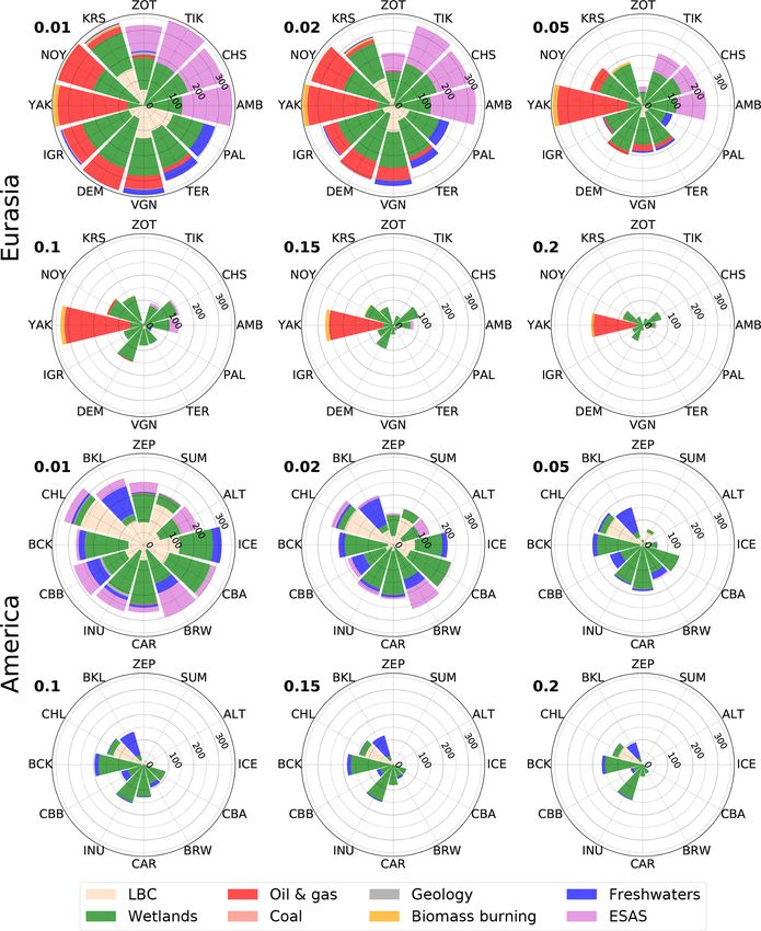
Figures 4 and S1–S23 show the time series of the direct con- aforementioned, including this sink in the regional simula-
tribution of each source and sink to the total δ 13 CCH4 at the tion will not change significantly our conclusions on the local
24 northern latitude stations. A focus is put on Zeppelin sta- source detectability.
tion in Fig. 4 because a new Aerodyne instrument has been
installed there during Summer 2018 in order to continuously 3.3 Detectability of northern high-latitude sources
measure δ 13 CCH4 for at least 1 year. Figure 4 illustrates the using isotopic measurements
magnitude and timing of the maximum signal of each source
during the year, the potential compensation between sources, The magnitude of δ 13 CCH4 signals to be expected at present
and the seasonality of the various contributions. and potential measurement sites and the contributions of in-
Zeppelin is a typical example of a remote site. The dividual sources to these signals do not lead directly to quan-
δ 13 CCH4 values from anthropogenic emissions are very small tifying the detectability of individual sources, as the latter
(< 0.02 ‰, except for some particular events which concern also depends on the performances of the measuring instru-
the lightest isotopic signatures) because the source areas are ment. Here we focus on a detectability definition taken from
far from the station and tend to be cancelled out because a regional inversion point of view: regional inversion systems
the signals from oil and gas, and from coal have approxi- analyse daily signals and optimize sources depending on syn-
mately the same magnitude but opposite signs. The signal optic deviations of the observed signals compared to the sim-
from geological sources remains negligible being 1 order of ulated ones. Therefore, a measuring instrument is consid-
magnitude lower than anthropogenic sources. Only wetland ered to provide useful information to the inversion only if
emissions succeed to tear the signal away from the value of the synoptic variability of the atmospheric signal can be de-
the boundary conditions, from June to October, with synoptic tected. To that end, we compute detectability capability in
changes up to −0.2 ‰. Freshwater systems intensify the sig- Fig. 5 and Table 4 as follows: (1) we compute the standard
nal by 0.02 ‰ on average in summer, with maxima around deviation over a 5 d running window of the simulated total
0.05 ‰ on a synoptic basis. These contributions are dimin- isotopic signal; (2) for a set of instrument precision thresh-
ished by biomass burning (∼ +0.01 ‰) and also by the frac- old (from 0.2 ‰ to 0.01 ‰, see Fig. 5 and Table 4), if the
tionating effects of the two major sinks (∼ +0.01 ‰). The running standard deviation is higher than the corresponding
simulated δ 13 CCH4 signal at the site is the result of these threshold, the source with the higher running standard devi-
competing signals. Varying the isotopic signatures of natu- ation for the same 5 d window is considered detected for that
ral sources does not change the conclusions with wetland, one day; (3) for each threshold, we count the number of days
freshwater, and ESAS synoptic events reaching at maximum over the year that each source is detected. Although the to-
−0.3 ‰, −0.1 ‰, and −0.15 ‰, respectively . Therefore, in tal atmospheric signal integrates contributions from different
the case of a remote station such as ZEP, signals of individual sources with different isotopic signatures, we keep only the
sources remain below 0.3 ‰ at the synoptic scale, and partial major source contributing to the signal as a 1st-order signal.
compensation between sources determines the total δ 13 CCH4 The range of instrument precision threshold was chosen
anomaly. according to present isotopic instrument systems. The flask
Analysing other stations (Figs. S1–S23) reveals that syn- measurements used in Sect. 3.1 (Table 1, Figs. 1 and 2) have
optic events larger than 2 ‰ due to summer wetland emis- an uncertainty of about 0.1 ‰. They were obtained using
sions could happen at AMB, BCK, CHS, DEM, IGR, INU, GC–IRMS (gas chromatography–isotope ratio mass spec-
NOY, and TIK. For freshwater emissions, events larger than trometry; White et al., 2018). Using continuous-flow isotope
0.5 ‰ are simulated at AMB, BKL, BRW, BCK, CBB, CHL ratio mass spectrometry, Fisher et al. (2006) reached a preci-
and INU. For ESAS, varying the isotopic signature induces sion of 0.05 ‰. Laser-based instruments, using cavity ring-
synoptic events larger than 0.3 ‰ at some sites (AMB, BRW, down spectrometry or direct absorption spectrometry (Nel-
CHS, and TIK). When varying the isotopic signature of an- son et al., 2004), have been developed since 10 years for
thropogenic emissions, DEM, IGR, KRS, NOY, and VGN CO2 isotopes (McManus et al., 2010) and, more recently for
show synoptic events due to oil and gas that are larger than methane (Santoni et al., 2012). The Aerodyne QCL instru-
0.15 ‰, and only YAK shows synoptic events due to fugitive ment has proven to be capable of high-frequency (≥ 1 Hz)
emissions larger than 1 ‰; these events occur mainly in win- measurements of 12 CH4 and 13 CH4 isotopes of CH4 with in
ter. Biomass burning synoptic events are the largest at BCK, situ 1 s rms δ 13 CCH4 precision of 1.5 ‰ and an Allan mini-
DEM, KRS, NOY, and YAK with events larger than 0.2 ‰. mum precision of 0.2 ‰ at 100 s (Santoni et al., 2012), re-
cently improved to 0.1 ‰ through laser stability improve-
Atmos. Chem. Phys., 19, 12141–12161, 2019 www.atmos-chem-phys.net/19/12141/2019/You can also read