Asthenospheric anelasticity effects on ocean tide loading around the East China Sea observed with GPS - Solid Earth
←
→
Page content transcription
If your browser does not render page correctly, please read the page content below
Solid Earth, 11, 185–197, 2020
https://doi.org/10.5194/se-11-185-2020
© Author(s) 2020. This work is distributed under
the Creative Commons Attribution 4.0 License.

Asthenospheric anelasticity effects on ocean tide loading around the
East China Sea observed with GPS
Junjie Wang1,2 , Nigel T. Penna2 , Peter J. Clarke2 , and Machiel S. Bos3
1 Department
           of Geomatics Engineering, Minjiang University, Fuzhou, China
2 School
       of Engineering, Newcastle University, Newcastle upon Tyne, UK
3 SEGAL, University of Beira Interior, Covilhã, Portugal

Correspondence: Junjie Wang (wangjunjie.gnss@qq.com)

Received: 21 August 2019 – Discussion started: 10 September 2019
Revised: 20 December 2019 – Accepted: 9 January 2020 – Published: 14 February 2020

Abstract. Anelasticity may decrease the shear modulus of           OTL displacements can reach several centimetres in the ver-
the asthenosphere by 8 %–10 % at semidiurnal tidal peri-           tical component and more than 1 cm in the horizontal com-
ods compared with the reference 1 s period of seismolog-           ponents, with the Earth’s response to the OTL depending
ical Earth models. We show that such anelastic effects are         strongly on the material properties within its interior (Far-
likely to be significant for ocean tide loading displacement at    rell, 1972). In the past 2 decades, Global Positioning Sys-
the M2 tidal period around the East China Sea. By compari-         tem (GPS) data analysis techniques have been developed to
son with tide gauge observations, we establish that from nine      directly measure OTL displacements with millimetre accu-
selected ocean tide models (DTU10, EOT11a, FES2014b,               racy and even submillimetre accuracy at some frequencies
GOT4.10c, HAMTIDE11a, NAO99b, NAO99Jb, OSU12,                      (e.g. Allinson et al., 2004; Thomas et al., 2007; Yuan et al.,
and TPXO9-Atlas), the regional model NAO99Jb is the most           2009; Penna et al., 2015). With parallel substantial advance-
accurate in this region and that related errors in the predicted   ments in the accuracy of global ocean tide models (Stammer
M2 vertical ocean tide loading displacements will be 0.2–          et al., 2014; Ray et al., 2019), comparisons of GPS-observed
0.5 mm. In contrast, GPS observations on the Ryukyu Is-            and predicted (modelled) OTL displacements have several
lands (Japan), with an uncertainty of 0.2–0.3 mm, show 90th-       times revealed the deficiencies of using spherically symmet-
percentile discrepancies of 1.3 mm with respect to ocean tide      ric, non-rotating, elastic, and isotropic (SNREI) Earth mod-
loading displacements predicted using the purely elastic ra-       els. One of the reasons for these deficiencies is that these
dial Preliminary Reference Earth Model (PREM). We show             models have been derived from seismic data and represent
that the use of an anelastic PREM-based Earth model re-            the Earth’s elastic properties at a reference period of 1 s but
duces these 90th-percentile discrepancies to 0.9 mm. Use of        have typically been assumed to be directly applicable at tidal
an anelastic radial Earth model consisting of a regional av-       frequencies.
erage of the laterally varying S362ANI model reduces the              Ito et al. (2009) found the average amplitude ratios be-
90th-percentile to 0.7 mm, which is of the same order as the       tween GPS tidal displacement observations and an Earth
sum of the remaining errors due to uncertainties in the ocean      tidal model (including OTL and Earth body tide) across
tide model and the GPS observations.                               Japan were greater than 1, indicating observational agree-
                                                                   ment with inelastic Earth models. Ito and Simons (2011)
                                                                   further attempted to invert GPS-observed displacements
                                                                   for one-dimensional profiles of the elastic moduli and
1   Introduction                                                   density beneath the western United States, demonstrating
                                                                   the limitations of the Preliminary Reference Earth Model
The periodic redistribution of ocean mass around the Earth’s       (PREM) (Dziewonski and Anderson, 1981). Also, Yuan and
surface due to ocean tides deforms the solid Earth, a phe-         Chao (2012) and Yuan et al. (2013) reported continental-
nomenon known as ocean tide loading (OTL). The resulting

Published by Copernicus Publications on behalf of the European Geosciences Union.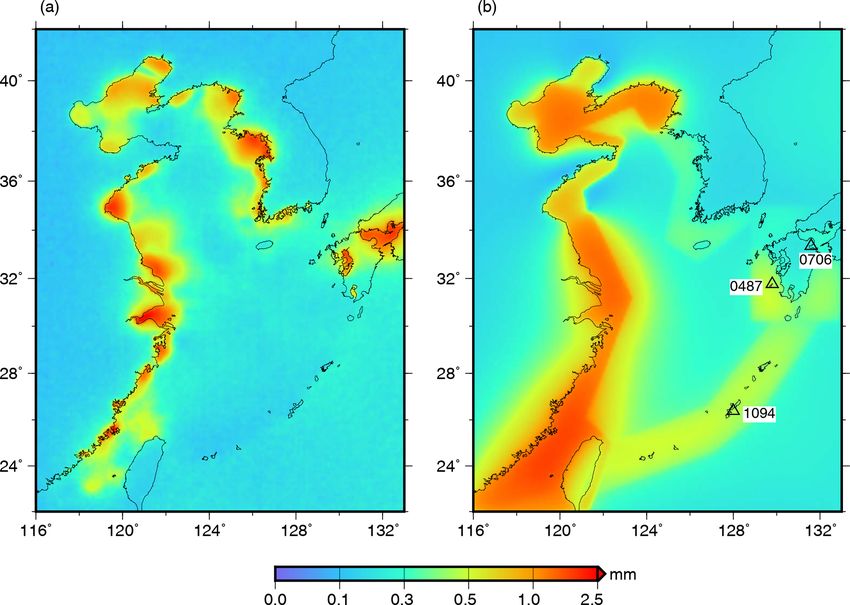
186                                           J. Wang et al.: Asthenospheric anelasticity effects around the East China Sea

scale spatially coherent differences between GPS-observed          ern Greenland, eastern Africa, and western Central America,
and predicted OTL displacements at sites located more than         are poorly sampled with continuously operating GPS net-
150 km inland from the coastline and attributed these dif-         works. However, the East China Sea (ECS) region exhibits
ferences to elastic and inelastic deficiencies in the a priori     a favourable combination of large OTL displacements and
Earth body tide model. Subsequently, these GPS results were        fairly consistent ocean tide models across much of it, so the
used by Lau et al. (2017) to look for lateral variations in        detectability ratio here exceeds 3 across a wide area and con-
body tide models of the lower mantle. For western Europe,          tains a healthy distribution of long-running GPS sites (Fig. 1b
Bos et al. (2015) showed that large discrepancies exist be-        shows the 102 GPS sites used). Accordingly, we have se-
tween GPS-observed and modelled OTL displacements, aris-           lected this as a suitable region for an independent test of Bos
ing from disregarding anelastic dispersion in the astheno-         et al.’s (2015) conclusions. A further attraction of this region
sphere that occurs when the elastic constants of the Earth         for the testing of Earth models is that its position overlying a
model are modified to be applicable at tidal periods. Such an      subduction zone means that it represents a very different tec-
effect could bring about a reduction of around 8 %–10 % of         tonic setting to the mature passive margin in western Europe
the shear modulus in the asthenosphere at tidal frequencies.       studied by Bos et al. (2015).
In addition, Martens et al. (2016) observed spatial coherence         Figure 1c shows the predicted M2 vertical OTL displace-
among residual M2 OTL displacements across South Amer-             ments across the ECS region using the FES2014b ocean tide
ica, postulating deficiencies in the a priori SNREI Earth mod-     model (Carrère et al., 2016) and an elastic PREM Green’s
els.                                                               function. It can be seen that the M2 vertical OTL dis-
   Bos et al. (2015) showed the feasibility of representing the    placement amplitudes are as large as 20–25 mm around the
behaviour of the asthenosphere across an absorption band           Ryukyu Islands and on the southeast coast of China, so the
from seismic to tidal frequencies by a constant quality fac-       anelastic OTL displacement discrepancies would be expected
tor Q, which provides a rough transformation to account            to be about 2 mm and therefore detectable using GPS. Over-
for the anelastic dispersion effect. Hence, it can be postu-       all, the accuracy of recent ocean tide models is believed to
lated that the asthenosphere should always produce ∼ 8.5 %         be good, e.g. Stammer et al. (2014) show sub-centimetre M2
OTL displacement discrepancies with respect to a purely            root mean square (RMS) agreement between bottom pres-
elastic PREM-based Earth model, not only in western Eu-            sure observations and seven recent models in the deep oceans
rope where Bos et al. (2015) demonstrated this effect but          globally and additionally, the FES2014b model has been sug-
also all over the world. However, these discrepancies will not     gested as providing a clear advancement in global ocean tide
be equally observable in all localities, either because ocean      modelling (Ray et al., 2019). However, the fact that the tides
tide amplitudes are too small within the 50–250 km distance        in the ECS are large and complex owing to the irregular ge-
range from the analysis point that samples asthenospheric be-      ometry of the basin (Lefèvre et al., 2000) implies that careful
haviour or because regional uncertainties in ocean tide mod-       evaluation of the ocean tide models is still necessary in this
els are too large to be able to attribute any observed discrep-    region to ascertain the optimal model and thus minimize the
ancy to the Earth model. To identify regions where the find-       effect of errors in ocean tide models on the OTL predictions.
ings of Bos et al. (2015) are testable, we have examined the          In this paper, we first assess the accuracy of a selection of
global distribution of a “detectability ratio”. This is defined    up-to-date ocean tide models in the ECS and quantify their
as the ratio between the elastic–anelastic OTL displacement        contribution to the predicted OTL error budget. We then de-
discrepancy (taken to be the difference between OTL pre-           scribe the kinematic GPS analysis approach for obtaining the
dicted using a purely elastic PREM Green’s function, as de-        observed OTL displacements. Finally, we examine the evi-
scribed in Sect. 3, and that using Bos et al.’s (2015) anelastic   dence of asthenospheric anelasticity effects in the ECS re-
S362ANI(M2 ) Green’s function) as the numerator and the            gion based on the GPS-observed OTL displacements. We
combination of expected GPS observational and ocean tide           consider the M2 constituent and the vertical component of
model related errors as the denominator. For the latter, the       OTL displacement, as these are dominant in the ECS region.
ocean tide model related error is characterized as the stan-
dard deviation (SD) of the predicted elastic OTL displace-
ments at each location, using each of the DTU10, EOT11a,           2   Ocean tide model accuracy assessment using tide
FES2014b, GOT4.10c, HAMTIDE11a, NAO99b, OSU12,                         gauges
and TPXO9-Atlas numerical ocean tide models (see Table 1
for references). The GPS observational error is assigned a SD      A prerequisite for using GPS measurements of OTL dis-
of 0.3 mm following Penna et al. (2015), which assumes that        placement for evaluating the Earth’s interior material proper-
at least 2.5 years of continuous GPS data will be available.       ties is that the impact of ocean tide model errors on the pre-
   Figure 1a shows a global 1/8◦ grid of detectability ratio       dicted OTL displacement is understood and found to be near
for the M2 vertical OTL displacement, which is unfavourable        negligible. Therefore, we first evaluate the quality of ocean
(less than 1) for most inland and deep ocean regions. Many of      tide models in the ECS region (considered throughout this
the areas where it exceeds 1, such as off the coasts of south-     paper as 116 to 133◦ E in longitude and 23 to 42◦ N in lati-

Solid Earth, 11, 185–197, 2020                                                               www.solid-earth.net/11/185/2020/
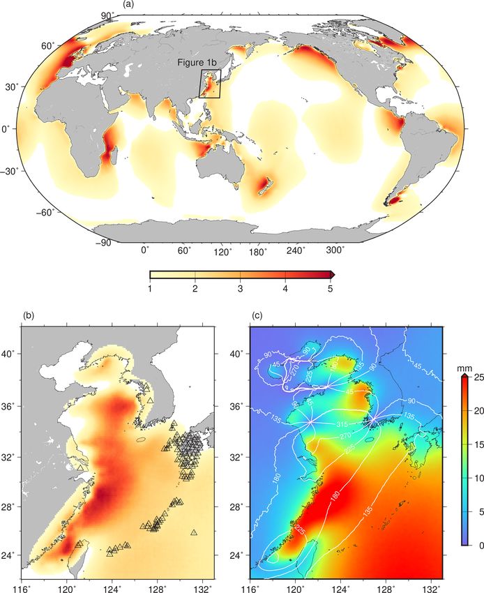
J. Wang et al.: Asthenospheric anelasticity effects around the East China Sea                                                         187

Figure 1. (a) Global distribution (1/8◦ grid) of M2 “detectability ratio” of the difference between vertical OTL displacements predicted
using purely elastic and anelastic Green’s functions, to uncertainty in residual OTL displacements predicted using eight ocean tide models
and the GPS observational error. (b) Detectability ratio in the East China Sea (ECS) region, showing the GPS sites used in this study as
triangles. The colour scale is the same as in (a). (c) The M2 vertical OTL displacement amplitudes and Greenwich phase lags for a 1/8◦ grid
across the ECS region using the FES2014b ocean tide model and an elastic PREM Green’s function.

tude) by assessing their consistency with each other and by             Envisat, and ICESat altimetry satellites, as well as tide gauge
comparing them with tide gauge observations.                            data. FES2014b, HAMTIDE11a, NAO99b, and TPXO9 are
   To date, no single ocean tide model has been demonstrated            barotropic data-assimilative models. DTU10 and EOT11a
as optimal in all regions of the world (Stammer et al., 2014;           are both based on an empirical correction to the global hy-
Ray et al., 2019), so we selected eight recent global models            drodynamic tide model FES2004 (Lyard et al., 2006), while
(DTU10, EOT11a, FES2014b, GOT4.10c, HAMTIDE11a,                         the a priori model for GOT4.10c is a collection of global and
NAO99b, OSU12, TPXO9-Atlas) and one regional model                      regional models blended at mutual boundaries. OSU12 is a
(NAO99Jb) for the quality assessment. The key features of               purely empirical model determined by an analysis of multi-
the models are listed in Table 1. All models, except for                mission satellite altimeter measurements. TPXO9-Atlas is
GOT4.10c, directly assimilate TOPEX/Poseidon (T/P) al-                  obtained by combining the base global TPXO9 and local so-
timeter data plus, for some of the models, data from one or             lutions for all coastal areas including around Antarctica and
more of the ERS-1/2, Geosat Follow-On (GFO), Jason-1/2,                 the Arctic Ocean. The regional model, NAO99Jb, covers the

www.solid-earth.net/11/185/2020/                                                                       Solid Earth, 11, 185–197, 2020
188                                           J. Wang et al.: Asthenospheric anelasticity effects around the East China Sea

area from 110 to 165◦ E in longitude and from 20 to 65◦ N          explained by the fact that the FES2004 model, on which
in latitude, including the whole area of our considered ECS        DTU10 and EOT11a are both based, has several grossly
region, and assimilates more local tide gauge data than do the     incorrect tidal values in this area owing to the insufficient
other models.                                                      satellite altimetry data available at the time. Such problems
   To evaluate the consistency among the different ocean tide      with the earlier set of finite element solution (FES) ocean
models for the dominant M2 constituent, all models were bi-        tide models were also seen from tidal gravity observations
linearly interpolated onto a common 1/16◦ grid across the          in Wuhan, China (Baker and Bos, 2003), near this subarea.
ECS region, and the SDs of the phasor differences from the         RMS agreements of better than 4 cm between tide gauge
mean were computed per grid point using Eq. (2) of Stam-           observations and each of the models are obtained for the
mer et al. (2014) and are shown in Fig. 2. It can be seen          Ryukyu Islands subarea, except for TPXO9-Atlas. This is
that away from the coastlines, all models are quite similar        despite TPXO9-Atlas having the finest resolution among
with the SDs no more than 1–2 cm, which likely arises be-          the models (1/30◦ ), whereas the coarser (1/2◦ ) GOT4.10c
cause they have more or less assimilated the same altimeter        and NAO99b models have better than 4 cm RMS agree-
data, albeit over different durations. However, closer to the      ment. Around the island of Kyushu, the observations com-
coast large intermodel discrepancies arise, especially in the      pare consistently well with FES2014b and NAO99Jb (RMS
Seto Inland Sea and near the coast of eastern China and the        lower than 4 cm), while the comparisons are poor for DTU10,
western Korean Peninsula, where the SD exceeds 30 cm in            EOT11a, HAMTIDE11a, OSU12, and TPXO9-Atlas along
places. To check if the large discrepancies are caused by the      the west coast of Kyushu and for GOT4.10c and NAO99b
older models, we considered the three most recent models           along the north coast of Kyushu. NAO99Jb exhibits the best
(FES2014b, GOT4.10c, and TPXO9-Atlas) and computed                 agreement with the observations in the Ariake Sea and Seto
the differences per pair of FES2014b-GOT4.10c, FES2014b-           Inland Sea, which is expected as it assimilates data from
(TPXO9-Atlas), and GOT4.10c-(TPXO9-Atlas). However,                219 local tide gauges (Matsumoto et al., 2000). This also
similar patterns and size of errors as in Fig. 2 were obtained     results in NAO99Jb being more accurate than NAO99b in
with the modern model difference pairs. The only changes           most parts of the ECS region. However, the agreement be-
were that the intermodel differences for the more modern           tween NAO99Jb and the tide gauges is no better than the
models tend to tail off slightly more rapidly on moving away       other models in the Kanmon Straits, because the tide gauges
from the coast of eastern China.                                   there were installed in 2011, after the release of NAO99Jb,
   To ascertain which models are the causes of the large SDs       and hence none of their data have been assimilated. Nonethe-
in some subareas and to assess their accuracy, we compared         less, NAO99Jb is the most accurate ocean tide model in the
each model with observations from 75 coastal tide gauges (58       ECS region as a whole.
from the Japan Oceanographic Data Center and 17 from the
University of Hawaii Sea Level Center) in the ECS region,
as shown in Fig. 2. Unfortunately no tide gauge data are cur-      3   Impact of ocean tide model errors on OTL
rently available within the Korea subarea. Using the UTide             displacement
package (Codiga, 2011), the tidal constants observed at these
locations were deduced from hourly sea level time series           In this section we assess the impact of ocean tide model er-
spanning 4 to 69 years, with a median time-series length of        rors on the predicted OTL displacements, which is needed to
26 years. For time series shorter than 18.6 years, we applied      ensure the confident geophysical interpretation of the GPS-
nodal corrections during the harmonic tidal analysis (Fore-        observed OTL displacement residuals considered thereafter.
man et al., 2009). The observed tidal constants are listed in      For a particular tidal constituent, the OTL displacement u at
Table S1 in the Supplement.                                        a point r on the Earth’s surface may be computed (predicted)
   In order to investigate in detail the problematic coastal ar-   with the following convolution integral (Farrell, 1972):
eas of eastern China, the western Korean Peninsula, and the                  Z
Seto Inland Sea, the region is divided into the separate sub-      u (r) =       ρG r − r 0 Z r 0 d,

                                                                                                                              (1)
areas shown in Fig. 2, basically in accordance with the zones

of intermodel discrepancy. Moreover, for the sake of describ-
ing the ocean tide model errors as precisely as possible in the    where  represents the global water areas, ρ is the density of
next section, the subarea denoted as Kyushu is further di-         seawater, G is a Green’s function that describes the displace-
vided. The M2 phasor difference between each model and             ment at r from a unit point load, and Z is the tide height at
each tide gauge was computed, and the RMS of these differ-         r 0 , written as a complex number to include both the ampli-
ences per model for all tide gauges in each subarea is listed      tude and varying phase lag. Here, the convolution integral is
in Table 2.                                                        determined by numerical integration and may be written as
   For eastern China, FES2014b and NAO99Jb perform quite
well (RMS of 10–12 cm), whereas DTU10 and EOT11a                   u (r) =
                                                                              X
                                                                                 ρZi Gi ,                                     (2)
are the worst models (RMS of 47–59 cm). This could be

Solid Earth, 11, 185–197, 2020                                                               www.solid-earth.net/11/185/2020/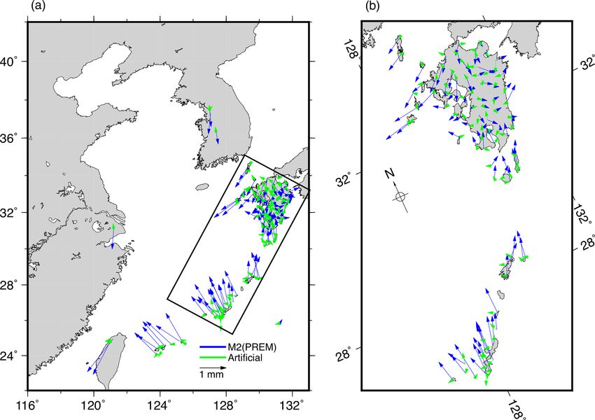
J. Wang et al.: Asthenospheric anelasticity effects around the East China Sea                                                                              189

Table 1. Summary of the selected ocean tide models.

              Model                  Data assimilateda                                 Resolution        Typeb       Author/reference
              DTU10                  T/P, ERS-2, GFO, Jason-1/2, Envisat                      1/8◦       E           Cheng and Andersen (2011)
              EOT11a                 T/P, ERS-2, Jason-1/2, Envisat                           1/8◦       E           Savcenko and Bosch (2012)
              FES2014b               T/P, ERS-1/2, Jason-1/2, Envisat, TG                    1/16◦       H           Carrère et al. (2016)
              GOT4.10c               ERS-1/2, GFO, Jason-1/2, ICESat                          1/2◦       E           Ray (2013)
              HAMTIDE11a             T/P, Jason-1                                             1/8◦       H           Taguchi et al. (2014)
              NAO99b                 T/P                                                      1/2◦       H           Matsumoto et al. (2000)
              NAO99Jb                T/P, TG                                                 1/12◦       H           Matsumoto et al. (2000)
              OSU12                  T/P, GFO, Jason-1, Envisat                               1/4◦       E           Fok (2012)
              TPXO9-Atlas            T/P, ERS-1/2, Jason-1/2, Envisat, TG                    1/30◦       H           Egbert and Erofeeva (2002)
            a T/P, TOPEX/Poseidon; GFO, Geosat Follow-on; TG, tide gauge. b E, empirical adjustment to an adopted a priori model; H, assimilation into a
            barotropic hydrodynamic model.

Figure 2. The M2 standard deviations for nine ocean tide models (DTU10, EOT11a, FES2014b, GOT4.10c, HAMTIDE11a, NAO99Jb,
NAO99b, OSU12, and TPXO9-Atlas). Panel (a) shows the whole East China Sea (ECS) region, while (b) is an enlargement of the Kyushu
subarea of (a). The white labelled polygons define the subareas for which the quality of the ocean tide models has been evaluated, and the
white dots represent the locations of coastal tide gauges.

where Gi here is the integrated Green’s function for the ith                          els (NAO99Jb was augmented globally outside its boundary
element of , as per Agnew (1997), and the tidal heights                              by FES2014b) using the SPOTL (NLOADF) software ver-
Zi are represented over  by inputting a global ocean tide                            sion 3.3.0.2 (Agnew, 1997). A Green’s function computed
model.                                                                                based on the isotropic, purely elastic version of PREM was
   Bos et al. (2015) took the SD of predicted OTL displace-                           input (as for all elastic PREM-generated results in this paper)
ments computed per point for a set of ocean tide models                               and is provided in Table S3 in the Supplement. As the GPS
as the error contribution of the ocean tide models in west-                           sites considered in this study are on land, the upper 3 km wa-
ern Europe, assuming that there were no systematic biases                             ter layer in PREM was replaced with the density and elastic
shared by the models. However, we have shown in Sect. 2                               properties from the underlying rock layer. The OTL displace-
that for the ECS region, the SD among the models is not al-                           ment SDs among the models per point are shown in Fig. 3a,
ways a good indicator of their accuracy. To check this, M2                            and it can be seen that the distribution of the SDs is simi-
vertical OTL displacements were computed for a 1/8◦ grid                              lar to those shown for the ocean tide models in Fig. 2, with
across the ECS region for each of the nine ocean tide mod-                            large SDs of up to 2.5 mm arising around eastern China, the

www.solid-earth.net/11/185/2020/                                                                                             Solid Earth, 11, 185–197, 2020
190 J. Wang et al.: Asthenospheric anelasticity effects around the East China Sea
Table 2. The root mean square (in centimetres) of the M2 phasor differences between each of the nine ocean tide models and the tide gauge
observations in each defined subarea of the East China Sea region.
Area DTU10 EOT11a FES2014b GOT4.10c HAMTIDE11a NAO99Jb NAO99b OSU12 TPXO9-Atlas
Eastern China 47.4 59.1 9.6 30.1 42.5 11.7 35.4 18.3 34.5
Ryukyu Islands 3.1 3.2 3.1 3.9 3.4 2.4 3.9 3.6 11.0
KyushuW 15.3 19.0 3.3 6.6 17.5 3.7 6.8 13.8 8.1
Ariake Sea 29.6 29.1 29.2 46.5 34.8 3.1 34.8 39.6 23.7
KyushuE 3.6 3.7 2.5 4.8 4.0 3.0 5.6 3.9 4.6
KyushuN 2.9 3.0 1.8 8.2 2.7 2.1 7.3 5.8 6.6
Seto Inland Sea 34.4 43.0 31.3 42.1 57.3 3.3 46.3 36.3 38.0
Kanmon Straits 15.6 17.6 14.5 12.9 16.8 16.2 16.8 11.8 11.9
western Korean Peninsula, and the Seto Inland Sea. How- of FES2014b for these areas, in accordance with the largest
ever, as shown in Sect. 2, these large SDs arise from large RMS model differences of 0.66 cm for deep oceans inferred
errors in some (but not all) of the nine ocean tide models, and by Stammer et al. (2014).
NAO99Jb was shown to be the most accurate model across Using Eq. (4) and inputting the NAO99Jb RMS errors per
the ECS region. Therefore, it is unreasonable to use the inter- subarea, the M2 vertical OTL displacement errors at each
model SD as an indicator of OTL displacement accuracy for point of a 1/8◦ grid were computed and are shown in Fig. 3b.
all of the ECS region. Instead, we now present an approach It can be seen that the largest errors of 1–2 mm are for the
which allows us to quantify (to the first order) the resulting points falling within the eastern China subarea, but these can
OTL displacement prediction error individually for a partic- be explained by the NAO99Jb model having a fairly large as-
ular ocean tide model. sumed RMS error of 11.7 cm for this subarea, and this has
Assuming the ocean is divided into k specified water areas the largest influence on the OTL displacement there. This
k (e.g as per Table 2) and that the ocean tide model error is, however, likely very conservative and results in errors for
magnitude per area is δk , the corresponding OTL accuracy much of the eastern China subarea that are too large, because
δuk is it can be seen from Figs. 2 and 3 that it is only very close to
X the coast where large intermodel discrepancies arise. Away
δuk (r) = ρδk Gi . (3) from the coast much of the intermodel ocean tide agree-
k ments for the eastern China subarea are about 2 cm. For the
Then, assuming no correlation between each of the k areas, rest of the ECS region, notably where most of the GPS sites
the total OTL displacement prediction error may be com- are located, the OTL errors arising from NAO99Jb model
puted as RMS errors are no more than ∼ 0.5 mm, even for sites on
the east of Kyushu where the intermodel OTL SDs are large
qX
(∼ 2.5 mm).
δu (r) = δu2k (r). (4)
To provide a more detailed indication of the influence on
Note that in practice there are likely to be negative correla- the OTL of the NAO99Jb ocean tide model errors from each
tions between adjacent water areas, which will result in the of the defined subareas, three GPS sites (0487, 0706, and
error estimates from Eq. (4) being too large (conservative). 1094) are considered, located on the east and west sides of
To evaluate the OTL error using Eq. (4) for NAO99Jb, the Kyushu and on the Ryukyu Islands, respectively (Fig. 3b).
most accurate ocean tide model in the ECS region, we define The contribution of each subarea to both the OTL displace-
the ocean tide model errors for the separate subareas (as per ment and its accompanying error are shown in Table 3, which
Fig. 2) as the RMS difference between NAO99Jb and the tide provides further clarification that the local ocean tides are the
gauge observations within the subarea (Table 2). For the Ko- principal contributor to the OTL displacements, as well as
rean subarea, although no tide gauge data source is available, the OTL errors. The large effect from the “other water ar-
the error of NAO99Jb for Korea can be estimated as the mean eas” is mainly due to their vast area, although most of this is
value of the RMS of the areas around Kyushu excluding the far from our study area and will have no impact on regional
Kanmon Straits, considering the fact that NAO99Jb also as- comparison of Earth models. The Kanmon Straits and east-
similated the tide gauge data around the Korean Peninsula. ern China, where NAO99Jb performs relatively poorly, have
The “other water areas” (comprising the central ECS sub- little effect on the OTL displacements at these sites, with
area and all other global water areas not named in Fig. 2) are contributions to the OTL amplitude and error of only 1.0–
either open oceans or narrow coastal areas that are far from 1.5 mm and less than 0.1 mm, respectively. Furthermore, the
the ECS. To be conservative, a slightly larger value of 0.7 cm effect of the ocean tide model errors from these two subareas
is chosen as the RMS error of NAO99Jb and its complement is no more than 0.13 mm for all three sites. These computa-
Solid Earth, 11, 185–197, 2020 www.solid-earth.net/11/185/2020/J. Wang et al.: Asthenospheric anelasticity effects around the East China Sea 191
Figure 3. (a) The standard deviation of M2 vertical OTL displacements, computed using the nine ocean tide models and an elastic PREM
Green’s function. (b) The M2 vertical OTL errors per grid point according to Eq. (4), using the RMS errors in NAO99Jb based on comparisons
with tide gauges and an elastic PREM Green’s function. The triangles (and accompanying names) denote GPS sites which are considered for
detailed OTL computation analysis.
Table 3. The contribution of the defined water subareas in Fig. 2 4 Kinematic GPS estimation of OTL displacement
to the M2 vertical OTL displacement amplitudes and the resulting
errors at GPS sites 0487, 0706, and 1094 according to Eq. (4), using Using the NASA GNSS-Inferred Positioning System
the NAO99Jb model and its RMS errors. (GIPSY) software in kinematic precise point positioning
(PPP) mode, Penna et al. (2015) showed for sites in western
Area M2 vertical OTL amp M2 vertical OTL error
(millimetres) (millimetres) Europe with at least 2.5 years of GPS data (4 years recom-
mended) that vertical OTL displacements may be estimated
0487 0706 1094 0487 0706 1094
with a precision of about 0.2–0.4 mm. We apply the same
Eastern China 1.18 0.99 1.48 0.11 0.09 0.13 approach for GPS sites in the ECS region. In order to assess
Ryukyu Islands 1.67 0.92 9.46 0.07 0.04 0.42
the accuracy and precision of the OTL displacements, par-
KyushuW 8.04 1.11 0.34 0.41 0.06 0.02
Ariake Sea 0.42 0.34 0.03 0.01 0.01 0.00 ticularly to check that the tuned coordinate and tropospheric
KyushuE 1.10 1.36 0.21 0.06 0.08 0.01 delay process noise values for western Europe are applica-
KyushuN 0.53 0.81 0.08 0.02 0.04 0.00 ble for the ECS region, we insert an artificial harmonic dis-
Seto Inland Sea 0.34 3.28 0.05 0.01 0.14 0.00 placement per GPS site. We then assess how well it is recov-
Kanmon Straits 0.00 0.01 0.00 0.00 0.00 0.00
Korea 0.18 0.15 0.13 0.02 0.01 0.00
ered from the kinematic PPP GPS processing, as per Penna
Other water areas 7.78 5.81 13.47 0.13 0.17 0.13 et al. (2015) but in the coordinate time series used for the fi-
nal OTL displacement estimation rather than as a preliminary
Total 18.33 10.54 22.53 0.46 0.25 0.46
investigation step.
4.1 GPS data source
tions were repeated for all the GPS sites, and only three of
the 102 GPS sites had a total OTL prediction error greater
All available continuous GPS data in the ECS region were
than 0.5 mm. It can therefore be concluded that the OTL dis-
collated for the window 2013.0–2017.0, with the distribution
placements computed using the NAO99Jb ocean model are
of the 102 sites used shown in Fig. 1. These comprised 96
suitable for investigating possible anelasticity effects in the
sites from the GPS Earth Observation Network (GEONET),
ECS region.
which all had at least 95 % data availability throughout the
4-year window considered and are located mainly on the
Ryukyu Islands and Kyushu. We also collated data from six
www.solid-earth.net/11/185/2020/ Solid Earth, 11, 185–197, 2020192 J. Wang et al.: Asthenospheric anelasticity effects around the East China Sea
International GNSS Service (IGS) sites in China and South analysis was then undertaken using UTide to estimate the
Korea, although two sites (SHAO and YONS) only had 2.5 residual M2 vertical OTL displacement signal per site, and
years of data. On the Ryukyu Islands and along the coast of also a 13.96 h harmonic was estimated to assess how well the
Kyushu, the sites exhibit detectability ratios of greater than introduced 3.0 mm amplitude artificial signal could be recov-
1, with the median value being 2.1, although close to the Seto ered. The resulting UTide formal errors were 0.1–0.2 mm.
Island Sea the ratio reduces to less than 1. The data spans of
at least 2.5 and typically 4 years are sufficient to separate the 4.3 Results
different major tidal constituents robustly according to the
Rayleigh criterion. The M2 vertical OTL residual phasors extracted from the har-
monic analysis are listed in Table S2 in the Supplement and
4.2 Data analysis strategy shown in Fig. 4, along with the artificial 13.96 h harmonic
signal residual phasors. It can be seen from Fig. 4 that on
Full details of the GPS data processing strategy used are the Ryukyu Islands and in the west coastal area of Kyushu
provided in Penna et al. (2015); in summary it is as fol- the M2 vertical OTL GPS-observed minus model discrep-
lows. Daily, 30 h, kinematic PPP GPS solutions were gener- ancies (residuals) can reach over 1.5 mm, corresponding to
ated for each site using GIPSY version 6.4 software with Jet about 7 % of the total loading signal. The typical magnitudes
Propulsion Laboratory (JPL) reprocessed version 2.1 fiducial of phasor differences between the recovered and original ar-
satellite orbits, Earth orientation parameters, and 30 s satel- tificial 13.96 h harmonic signals are 0.2–0.3 mm, providing
lite clocks held fixed in the IGb08 reference frame. A priori an indication of the accuracy level of our GPS-observed M2
hydrostatic and wet zenith tropospheric delays from the Eu- vertical OTL displacements and indicating that the optimal
ropean Centre for Medium-Range Weather Forecasts reanal- process noise values found for western Europe by Penna et
ysis products were used, with residual zenith tropospheric al. (2015) are also applicable to the ECS region. Since the
delays estimated every 5 min (applying a process noise of ocean tide error of NAO99Jb maps to only an error of 0.2–
0.1 mm s−1/2 ), together with north–south and east–west tro- 0.5 mm for the predicted M2 vertical OTL displacement val-
pospheric gradients. The VMF1 gridded mapping function ues across the Ryukyu Islands and Kyushu (Fig. 3b), it can be
was used with an elevation cut-off angle of 10◦ , and correc- concluded that the 1.5 mm discrepancies must be dominated
tions were applied for solid Earth and pole tides according by errors in the elastic PREM Green’s function.
to the International Earth Rotation Service (IERS) Conven-
tions 2010 (Petit and Luzum, 2010), along with IGS satellite
and receiver antenna phase centre variation corrections. Am- 5 Optimal Green’s function for the East China Sea
biguities were fixed to integers according to the approach of region
Bertiger et al. (2010). Receiver coordinates were estimated
every 5 min, with a coordinate process noise of 3.2 mm s−1/2 As Green’s functions essentially depend on the material
applied. OTL displacement was modelled using the IERS properties of the adopted Earth models, an improvement of
Conventions (2010) HARDISP.F routine, based on ampli- the agreement between GPS-observed and predicted OTL
tudes and phase lags generated using the NLOADF soft- values (reduction in the observational residuals) could be ex-
ware with the NAO99Jb model (augmented in the rest of pected by modifying the Earth models, and the representa-
the world with the FES2014b model) and a PREM elastic tion of the asthenosphere has been demonstrated to be es-
Green’s function, computed in the centre of mass of the solid pecially important (Bos et al., 2015). So far we have used
Earth and oceans (CM) frame to be compatible with the JPL Green’s functions computed from isotropic, purely elastic
orbits. In each daily solution, an artificial 13.96 h harmonic PREM, and we first consider whether the more recent elas-
signal of 3.0 mm amplitude was introduced in each of the tic S362ANI Earth model (Kustowski et al., 2008), which is
east, north, and vertical components, with the phase refer- a transversely isotropic seismic tomographic model for the
enced to zero defined at the GPS timeframe epoch J2000, and mantle, results in a reduction in the residuals. This model
hence the GPS harmonic estimation capability with the afore- provides horizontal and vertical shear velocities (transversely
mentioned GIPSY processing settings assessed. The value of isotropic) on a regular longitude–latitude grid for various
13.96 h was chosen as the period of this displacement follow- depths. For each depth layer between longitudes 122 and
ing Penna et al. (2015), as it is approximately in the semid- 133◦ E and latitudes 23 and 35◦ N, we computed averaged
iurnal band but is distinct from the main tidal harmonics, so shear velocities, which were used to compute the load Love
it will not be contaminated by geophysical signals. numbers following Bos and Scherneck (2013), together with
The estimated coordinates at 5 min resolution within the the density and compressional velocities of the STW105
central 24 h of the daily 30 h kinematic PPP GPS solutions model that was also developed by Kustowski et al. (2008).
(which ran from 21:00 UTC the previous day to 03:00 UTC It can be seen from Table 4 that using the elastic S362ANI
the next day) were averaged in nonoverlapping, 30 min bins Green’s function reduces the overall RMS of the residuals by
then concatenated to form coordinate time series. Harmonic about 0.1 mm compared to the elastic PREM Green’s func-
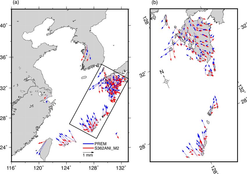
Solid Earth, 11, 185–197, 2020 www.solid-earth.net/11/185/2020/J. Wang et al.: Asthenospheric anelasticity effects around the East China Sea 193 Figure 4. Phasor differences (in blue) between the GPS-observed M2 vertical OTL displacements and the predictions computed using the NAO99Jb regional ocean tide model (augmented elsewhere globally with FES2014b) and an elastic PREM Green’s function. Also shown (in green) are the phasor differences between the recovered and original artificial ∼ 13.96 h harmonic vertical displacement signal of 3.0 mm amplitude. (a) Shows the whole ECS region, while (b) is an enlargement of Kyushu and part of the Ryukyu Islands, from the boxed region in (a). tion (and similarly for the maximum and 90th-percentile val- values reduce from 1.3 mm with PREM to 0.9 mm with ues), which could be explained by its use of the regional PREM_M2 and to ∼ 0.7 mm with S362ANI_M2. This re- mean shear velocity. duction across the Ryukyu Islands when using S362ANI_M2 We next considered whether using Green’s functions instead of PREM can be clearly seen in Fig. 5. However, with the anelastic dispersion effect in each of PREM and one can observe that the residual phasors for S362ANI_M2 S362ANI results in reductions in the residuals. The elastic still show some correlations along the Ryukyu Islands, which properties for these Earth models have been derived from might be due to the tectonic setting of the subduction zone. seismic observations and are valid at the reference period As residuals at the ∼ 0.7 mm level remain after account- of 1 s. To include the anelastic dispersion effect, the values ing for anelasticity effects with the regional S362ANI_M2 of the shear modulus were converted from a period of 1 s model, we also tested the optimality of the Green’s function to the period of the M2 harmonic using the relation formula by computing a range of Green’s functions based on different given by eq. (9.66) in Dahlen and Tromp (1998) with a con- asthenosphere depths and values of Q. For the density and stant absorption band, as described by Bos et al. (2015). The compressional velocity, S362ANI only provides global mean bulk modulus has a much higher-quality factor Q and is as- profiles. In our work, the asthenosphere is defined a priori to sumed not to be affected. After modifying the shear modulus, be between depths of 80 and 220 km with a Q of 70 as per the load Love numbers were computed as described in Bos Kustowski et al. (2008). Following a similar method to Bos and Scherneck (2013), and the respective anelastic Green’s et al. (2015), we vary the depths of the top (D1) and bottom functions will be hereafter referred to as PREM_M2 and (D2) of the asthenosphere of S362ANI and the amount of S362ANI_M2 (these, together with all the Green’s functions anelastic dispersion (Q) in this layer. For each combination used in this section, are listed in Tables S3 and S4 in the Sup- of these three parameters, a new Green’s function was com- plement). It can be seen from Table 4 that use of PREM_M2 puted via the load Love number formulation. While comput- and S362ANI_M2 reduces the overall RMS of the residu- ing the load Love numbers, we transformed the shear modu- als from ∼ 0.5 to ∼ 0.4 mm. However, if only the GPS sites lus from the reference period (1 s) to M2 as described above. on the Ryukyu Islands are considered, the RMS residual The Q value in the other layers is at least twice that of the is reduced from ∼ 0.7 mm with elastic PREM and elastic asthenosphere, so the frequency dependence will be smaller, S362ANI, to ∼ 0.5 mm with PREM_M2 and to ∼ 0.4 mm but to be consistent the elastic properties were also trans- with S362ANI_M2. The respective 90th-percentile residual formed to the period of harmonic M2 . However, these Q val- www.solid-earth.net/11/185/2020/ Solid Earth, 11, 185–197, 2020
194                                             J. Wang et al.: Asthenospheric anelasticity effects around the East China Sea

Table 4. Statistics (in millimetres) of the phasor differences between the GPS-observed and predicted M2 vertical OTL displacements using
the NAO99Jb regional ocean tide model (augmented elsewhere globally with FES2014b) and various Green’s functions. The label 90th
denotes the percentile.

                           Green’s function          The whole ECS region               Ryukyu Islands
                                                  Min    Max     90th    RMS     Min     Max    90th     RMS
                           PREM                   0.08   1.59    1.17     0.53   0.63    1.54   1.29     0.74
                           S362ANI                0.06   1.45    1.05     0.45   0.50    1.45   1.17     0.66
                           PREM_M2                0.10   1.12    0.86     0.41   0.25    1.12   0.89     0.47
                           S362ANI_M2             0.01   1.39    0.79     0.40   0.13    0.95   0.72     0.37
                           mod_S362ANI_M2         0.09   1.26    0.79     0.39   0.17    1.02   0.78     0.41

Figure 5. Phasor differences between our GPS-observed M2 vertical OTL displacements and the predictions computed using the NAO99Jb
regional ocean tide model (augmented elsewhere globally with FES2014b) and the elastic PREM (blue phasors) and S362ANI_M2 (red
phasors) Green’s functions. Panel (a) shows the whole ECS region, while (b) is an enlargement of Kyushu and part of the Ryukyu Islands,
for the boxed region in (a).

ues were not varied in our inversion. New Green’s functions             als statistics with this mod_S362ANI_M2 Green’s function
were then derived and used to predict the M2 vertical OTL               are practically identical to those using S362ANI_M2 (and
values using the NAO99Jb ocean tide model. This transfor-               although not shown, very similar patterns for the residuals
mation produces complex-valued shear moduli and therefore               arise as in Fig. 5), which confirms the large influence of the
complex-valued Green’s functions, but the imaginary part is             asthenosphere. In terms of practical usage for the region,
less than 5 % of the real part (Bos et al., 2015) and can be ne-        S362ANI_M2 with its correction of S362ANI for anelastic
glected. The optimal Green’s function was considered to be              dispersion provides a simple way to improve predicted OTL
that which minimized the sum of the squared misfits between             displacements instead of performing the complex numerical
the observed and predicted OTL phasor values using all the              optimization scheme each time. As a further simple practical
GPS sites. It was obtained when Q was 90 (corresponding to              implementation for the region, the global PREM_M2 leads
a reduction of the shear modulus of about 7.6 % at the M2               to almost comparable results as S362ANI_M2.
period), and the estimated values of D1 and D2 were 40 and                 As a further check on the explanation of the observed and
220 km, respectively, implying an asthenosphere extending               model discrepancies which we have attributed to astheno-
to shallower depths than its original definition for this region        spheric anelasticity, we used the CARGA programme (Bos
in S362ANI. It can be seen from Table 4 that the residu-                and Baker, 2005) to compute the effect of varying seawa-

Solid Earth, 11, 185–197, 2020                                                                    www.solid-earth.net/11/185/2020/
J. Wang et al.: Asthenospheric anelasticity effects around the East China Sea 195
ter density on the M2 vertical OTL displacements for the lowers the shear modulus by about 8 % in the asthenosphere,
102 GPS sites. First we computed the OTL displacements reduces the 90th-percentile discrepancies to 0.9 and 0.7 mm
using a constant global density of seawater of 1030 kg m−3 . for PREM and S362ANI, respectively. We estimated a re-
Then we recomputed the OTL displacements using the spa- gionally optimal Green’s function by varying the depth and
tially varying (0.25◦ × 0.25◦ ) mean column seawater den- thickness of the asthenosphere of the S362ANI Earth model
sity from the World Ocean Atlas (Boyer et al., 2013) and and its Q values, but this resulted in essentially no further
found the mean change in M2 vertical amplitude at our GPS reduction in the discrepancies.
sites was 0.03 mm (maximum difference of 0.16 mm). We This paper has confirmed the importance of considering
then also corrected the mean seawater density per column the asthenospheric anelasticity effects observed by Bos et
for compressibility according to Ray (2013) and found that al. (2015). It is necessary to incorporate dissipative effects
the mean change in M2 vertical OTL displacement amplitude for the Green’s functions based on seismic Earth models;
increased to 0.11 mm (maximum difference of 0.37 mm). use of elastic parameters at 1 s period is insufficient. The
Whilst such magnitude differences now have the potential to PREM_M2 Green’s function is near-optimal for the ECS re-
be detectable by geodetic observations, they are too small to gion and western Europe, and it represents a sensible com-
explain our observed 1.5 mm discrepancies. promise with global applicability, so it is therefore a prag-
matic choice for OTL prediction in geodetic analysis. For
sites in areas where the detectability ratio exceeds 1 as shown
6 Conclusions in Fig. 1a or where the highest accuracy is demanded, a re-
gional anelastic Green’s function calculated directly from a
By introducing the detectability ratio for the asthenospheric laterally varying Earth model such as S362ANI should be
anelasticity effects and considering the distribution of the considered.
available GPS sites, the ECS region was selected as a
potential area to observe the anelastic dispersion in the
asthenosphere. Using an intercomparison of eight recent Data availability. GPS data were obtained from the Crustal
global models (DTU10, EOT11a, FES2014b, GOT4.10c, Dynamics Data Information System, one of the International
HAMTIDE11a, NAO99b, OSU12, TPXO9-Atlas) and one GNSS Service data centres (ftp://cddis.nasa.gov/gnss/data/daily/,
regional (NAO99Jb) model and a validation with tide gauges, Crustal Dynamics Data Information System, 2016) and by re-
quest from the GPS Earth Observation Network (GEONET)
NAO99Jb has been demonstrated to be the most accurate tide
of the Geospatial Information Authority of Japan (GSI) (http:
model in the region. In the open sea areas NAO99Jb could be //datahouse1.gsi.go.jp/terras/terras_english.html, GSI, 2015). The
slightly worse than the other ocean tide models, due to the ocean tide models used were those provided in the SPOTL software
assimilation of more satellite altimetry data in the latter, but version 3.3.0.2 distribution (https://igppweb.ucsd.edu/~agnew/
this does not outweigh the benefits of forcing the NAO99Jb Spotl/spotlmain.html, Agnew, 2013), except that FES2014b
model to fit a large number of tide gauge observations. We was obtained from https://www.aviso.altimetry.fr/en/data/products/
quantified the impact of the errors in NAO99Jb on the pre- auxiliary-products/global-tide-fes.html (LEGOS, NOVELTIS, and
dicted OTL values, based on the RMS difference between CLS, 2016), OSU12 was obtained from https://geodesy.geology.
NAO99Jb and the tide gauge observations. Compared to the ohio-state.edu/oceantides/OSU12v1.0/readme1st.dat (Fok et al.,
approach of using the SD of predicted OTL displacements as 2012), TPXO9-Atlas was obtained from http://volkov.oce.orst.edu/
the error contribution of the ocean tide models, this method tides/tpxo9_atlas.html (Egbert and Erofeeva, 2019), and GOT4.10c
was provided by its author Richard Ray from the NASA God-
can allow for systematic biases shared by the models, so the
dard Space Flight Center via personal communication (2016).
outputs are more conservative. For the GPS sites located in
The Earth models were obtained from http://ds.iris.edu/ds/products/
Japan, the errors in NAO99Jb result in M2 vertical OTL dis- emc-referencemodels/ (IRIS DMC, 2011); JPL orbits clocks
placement errors of 0.2–0.5 mm. were obtained from https://sideshow.jpl.nasa.gov/pub/JPL_GPS_
We then estimated the M2 vertical OTL displacements for Products_IGb08/ (JPL, 2019); tide gauge data was obtained
102 sites around the ECS using GPS with typical accuracy of from the Japan Oceanographic Data Centre (https://www.jodc.go.
0.2–0.3 mm. On the Ryukyu Islands and in the west coastal jp/jodcweb/JDOSS/index.html, JODC, 2018) and the University
area of Kyushu, the discrepancies between GPS-observed of Hawaii Sea Level Center (ftp://ftp.soest.hawaii.edu/uhslc/rqds,
and predicted values can reach over 1.5 mm (1.3 mm 90th Caldwell et al., 2015).
percentile) when using the NAO99Jb tide model and the
purely elastic PREM Green’s function. The discrepancies
cannot be explained by the sum of the remaining errors due Supplement. The supplement related to this article is available on-
to ocean tide models and the uncertainty in the GPS obser- line at: https://doi.org/10.5194/se-11-185-2020-supplement.
vations themselves or by the small change in elastic param-
eters that results from using a regional average of the elas-
Author contributions. PJC, NTP, and JW devised the study. NTP
tic S362ANI model in place of PREM. However, modelling
undertook GIPSY processing of the GPS data. JW carried out the
of the anelastic dispersion effect using the Q values, which
www.solid-earth.net/11/185/2020/ Solid Earth, 11, 185–197, 2020196 J. Wang et al.: Asthenospheric anelasticity effects around the East China Sea
analysis of the tide gauge observations, ocean tide loading displace- Bos, M. S. and Baker, T. F.: An estimate of errors in grav-
ments, and GPS coordinate time series under the supervision of ity ocean tide loading computations, J. Geodesy, 79, 50–63,
NTP and PJC, and MSB computed the elastic and anelastic Green’s https://doi.org/10.1007/s00190-005-0442-5, 2005
functions. All authors contributed to the discussion of the results Bos, M. S. and Scherneck, H. G.: Computation of Green’s func-
and writing of the paper. tions for ocean tide loading, in: Sciences of Geodesy – II: In-
novations and Future Developments, edited by: Xu, G., Springer
Berlin Heidelberg, Berlin, Heidelberg, 1–52, 2013.
Competing interests. The authors declare that they have no conflict Bos, M. S., Penna, N. T., Baker, T. F., and Clarke, P. J.: Ocean
of interest. tide loading displacements in western Europe: 2. GPS-observed
anelastic dispersion in the asthenosphere, J. Geophys. Res.-Sol.
Ea., 120, 6540–6557, https://doi.org/10.1002/2015JB011884,
Special issue statement. This article is part of the special 2015.
issue “Developments in the science and history of tides Boyer, T. P., Antonov, J. I., Baranova, O. K., Coleman, C., Gar-
(OS/ACP/HGSS/NPG/SE inter-journal SI)”. It is not associ- cia, H. E., Grodsky, A., Johnson, D. R., Locarnini, R. A.,
ated with a conference. Mishonov, A. V., O’Brien, T. D., Paver, C. R., Reagan, J.
R., Seidov, D., Smolyar, I. V., and Zweng, M. M.: World
Ocean Database 2013, NOAA Atlas NESDIS 72, S. Levi-
tus, edited by: Mishonov, A., Silver Spring, MD, 209 pp.,
Acknowledgements. All data providers listed in the Data Availabil-
https://doi.org/10.7289/V5NZ85MT, 2013.
ity statement are thanked, as well as Duncan Agnew, Daniel Codiga,
Caldwell, P. C., Merrifield, M. A., and Thompson, P. R.: Sea level
and NASA JPL for providing the SPOTL, UTide, and GIPSY
measured by tide gauges from global oceans – the Joint Archive
software packages, respectively. The figures were generated using
for Sea Level holdings, Version 5.5, available at: ftp://ftp.soest.
the Generic Mapping Tools software (Wessel et al., 2013). Con-
hawaii.edu/uhslc/rqds (last access: 7 February 2020), 2015.
structive reviews and comments by Duncan Agnew, Richard Ray,
Carrère, L., Lyard, F., Cancet, M., Guillot, A., and Picot, N.: FES
Philip Woodworth, and an anonymous reviewer are appreciated.
2014, a new tidal model – Validation results and perspectives
for improvements, ESA living planet symposium, Prague, Czech
Republic, 9–13 May 2016, Paper 1956, 2016.
Financial support. This research has been supported by the Chi- Cheng, Y. C. and Andersen, O. B.: Multimission em-
nese Scholarship Council (grant no. 201606710069) and the UK pirical ocean tide modeling for shallow waters and
Natural Environment Research Council (grant no. NE/R010234/1). polar seas, J. Geophys. Res.-Oceans, 116, C11001,
https://doi.org/10.1029/2011jc007172, 2011.
Codiga, D.: Unified tidal analysis and prediction using the UTide
Review statement. This paper was edited by Philip Woodworth and Matlab functions, Graduate School of Oceanography, University
reviewed by Duncan Agnew, Richard Ray, and one anonymous ref- of Rhode Island, Narragansett, RI, Technical Report 2011-01,
eree. 59 pp., 2011.
Crustal Dynamics Data Information System: International GNSS
Service, Daily 30-second observation data, available at: ftp://
cddis.nasa.gov/gnss/data/daily/ (last access: 7 February 2020),
References 2016.
Dahlen, F. A. and Tromp, J.: Theoretical global seismology, Prince-
Agnew, D. C.: NLOADF: A program for computing ocean- ton University Press, New Jersey, USA, 1998.
tide loading, J. Geophys. Res.-Sol. Ea., 102, 5109–5110, Dziewonski, A. M. and Anderson, D. L.: Preliminary refer-
https://doi.org/10.1029/96jb03458, 1997. ence Earth model, Phys. Earth Planet. In., 25, 297–356,
Agnew, D. C.: SPOTL: Some Programs for Ocean-Tide Loading, https://doi.org/10.1016/0031-9201(81)90046-7, 1981.
available at: https://igppweb.ucsd.edu/~agnew/Spotl/spotlmain. Egbert, G. D. and Erofeeva, S. Y.: Efficient inverse mod-
html (last access: 7 February 2020), 2013. eling of barotropic ocean tides, J. Atmos. Ocean.
Allinson, C. R., Clarke, P. J., Edwards, S. J., King, M. A., Tech., 19, 183–204, https://doi.org/10.1175/1520-
Baker, T. F., and Cruddace, P. R.: Stability of direct GPS esti- 0426(2002)0192.0.CO;2, 2002.
mates of ocean tide loading, Geophys. Res. Lett., 31, L15603, Egbert, G. D. and Erofeeva, S. Y.: TPXO9-atlas, available at: http://
https://doi.org/10.1029/2004gl020588, 2004. volkov.oce.orst.edu/tides/tpxo9_atlas.html (last access: 7 Febru-
Baker, T. F. and Bos, M. S.: Validating Earth and ocean tide mod- ary 2020), 2019.
els using tidal gravity measurements, Geophys. J. Int., 152, 468– Farrell, W. E.: Deformation of the Earth by surface loads, Rev. Geo-
485, https://doi.org/10.1046/j.1365-246X.2003.01863.x, 2003. phys., 10, 761–797, https://doi.org/10.1029/RG010i003p00761,
Bertiger, W., Desai, S. D., Haines, B., Harvey, N., Moore, A. 1972.
W., Owen, S., and Weiss, J. P.: Single receiver phase am- Fok, H. S.: Ocean tides modeling using satellite altimetry, PhD the-
biguity resolution with GPS data, J. Geodesy, 84, 327–337, sis, The Ohio State University, USA, 187 pp., 2012.
https://doi.org/10.1007/s00190-010-0371-9, 2010. Fok, H. S., Shum, C. K., and Yi, Y.: The OSU12 Global Ocean
Tide Model, Version 1.0, available at: https://geodesy.geology.
Solid Earth, 11, 185–197, 2020 www.solid-earth.net/11/185/2020/J. Wang et al.: Asthenospheric anelasticity effects around the East China Sea 197 ohio-state.edu/oceantides/OSU12v1.0/readme1st.dat (last ac- Penna, N. T., Clarke, P. J., Bos, M. S., and Baker, T. F.: Ocean tide cess: 7 February 2020), 2012. loading displacements in western Europe: 1. Validation of kine- Foreman, M. G. G., Cherniawsky, J. Y., and Ballamtyne, matic GPS estimates, J. Geophys. Res.-Sol. Ea., 120, 6523–6539, V. A.: Versatile harmonic tidal analysis: improvements https://doi.org/10.1002/2015JB011882, 2015. and applications, J. Atmos. Ocean. Tech., 26, 806–817, Petit, G. and Luzum, B.: IERS conventions (2010), IERS, Frankfurt https://doi.org/10.1175/2008jtecho615.1, 2009. am Main, Germany, IERS Technical Note No. 36, 179 pp., 2010. GSI: Terms of service of GSI’s GNSS stations data, available Ray, R. D.: Precise comparisons of bottom-pressure and alti- at: http://datahouse1.gsi.go.jp/terras/terras_english.html (last ac- metric ocean tides, J. Geophys. Res.-Oceans, 118, 4570–4584, cess: 7 February 2020), 2015. https://doi.org/10.1002/jgrc.20336, 2013. IRIS DMC: Data Services Products: EMC-Reference Models, avail- Ray, R. D., Loomis, B. D., Luthcke, S. B., and Rachlin, K. E.: able at: http://ds.iris.edu/ds/products/emc-referencemodels/ (last Tests of ocean-tide models by analysis of satellite-to-satellite access: 7 February 2020), 2011. range measurements: an update, Geophys. J. Int., 217, 1174– Ito, T. and Simons, M.: Probing asthenospheric density, tempera- 1178, https://doi.org/10.1093/gji/ggz062, 2019. ture, and elastic moduli below the Western United States, Sci- Savcenko, R. and Bosch, W.: EOT11a – Global Empirical Ocean ence, 332, 947–951, https://doi.org/10.1126/science.1202584, Tide model from multi-mission satellite altimetry, Deutsches 2011. Geodätisches Forschungsinstitut (DGFI), München, Germany, Ito, T., Okubo, M., and Sagiya, T.: High resolution mapping of Earth DGFI Rep. No. 89, 49 pp., 2012. tide response based on GPS data in Japan, J. Geodyn., 48, 253– Stammer, D., Ray, R. D., Andersen, O. B., Arbic, B. K., Bosch, 259, https://doi.org/10.1016/j.jog.2009.09.012, 2009. W., Carrère, L., Cheng, Y., Chinn, D. S., Dushaw, B. D., Egbert, JODC: J-DOSS: JODC Data On-line Service System, available at: G. D., Erofeeva, S. Y., Fok, H. S., Green, J. A. M., Griffiths, S., https://www.jodc.go.jp/jodcweb/JDOSS/index.html (last access: King, M. A., Lapin, V., Lemoine, F. G., Luthcke, S. B., Lyard, 7 February 2020), 2018. F., Morison, J., Müller, M., Padman, L., Richman, J. G., Shriver, JPL: GNSS Science Data, available at: https://sideshow.jpl.nasa. J. F., Shum, C. K., Taguchi, E., and Yi, Y.: Accuracy assessment gov/ (last access: 7 February 2020), 2019. of global barotropic ocean tide models, Rev. Geophys., 52, 243– Kustowski, B., Ekström, G., and Dziewoński, A. M.: Anisotropic 282, https://doi.org/10.1002/2014RG000450, 2014. shear-wave velocity structure of the Earth’s mantle: A Taguchi, E., Stammer, D., and Zahel, W.: Inferring deep ocean global model, J. Geophys. Res.-Sol. Ea., 113, B06306, tidal energy dissipation from the global high-resolution data- https://doi.org/10.1029/2007JB005169, 2008. assimilative HAMTIDE model, J. Geophys. Res.-Oceans, 119, Lau, H. C. P., Mitrovica, J. X., Davis, J. L., Tromp, J., 4573–4592, https://doi.org/10.1002/2013JC009766, 2014. Yang, H.-Y., and Al-Attar, D.: Tidal tomography con- Thomas, I. D., King, M. A., and Clarke, P. J.: A comparison of strains Earth’s deep-mantle buoyancy, Nature, 551, 321–326, GPS, VLBI and model estimates of ocean tide loading displace- https://doi.org/10.1038/nature24452, 2017. ments, J. Geodesy, 81, 359–368, https://doi.org/10.1007/s00190- Lefèvre, F., Le Provost, C., and Lyard, F. H.: How can we improve 006-0118-9, 2007. a global ocean tide model at a regional scale? A test on the Yel- Wessel, P., Smith, W. H. F., Scharroo, R., Luis, J., and low Sea and the East China Sea, J. Geophys. Res.-Oceans, 105, Wobbe, F.: Generic Mapping Tools: Improved ver- 8707–8725, https://doi.org/10.1029/1999JC900281, 2000. sion released, EOS T. Am. Geophys. Un., 94, 409–410, LEGOS, NOVELTIS and CLS: FES (Finite Element Solution)- https://doi.org/10.1002/2013eo450001, 2013. Global tide, FES2014, available at: https://www.aviso.altimetry. Yuan, L. G. and Chao, B. F.: Analysis of tidal signals fr/en/data/products/auxiliary-products/global-tide-fes.html (last in surface displacement measured by a dense continu- access: 7 February 2020), 2016. ous GPS array, Earth Planet. Sc. Lett., 355, 255–261, Lyard, F., Lefèvre, F., Letellier, T., and Francis, O.: Modelling the https://doi.org/10.1016/j.epsl.2012.08.035, 2012. global ocean tides: modern insights from FES2004, Ocean Dy- Yuan, L. G., Ding, X. L., Zhong, P., Chen, W., and Huang, nam., 56, 394–415, https://doi.org/10.1007/s10236-006-0086-x, D. F.: Estimates of ocean tide loading displacements and 2006. its impact on position time series in Hong Kong using a Martens, H. R., Simons, M., Owen, S., and Rivera, L.: Obser- dense continuous GPS network, J. Geodesy, 83, 999–1015, vations of ocean tidal load response in South America from https://doi.org/10.1007/s00190-009-0319-0, 2009. subdaily GPS positions, Geophys. J. Int., 205, 1637–1664, Yuan, L. G., Chao, B. F., Ding, X. L., and Zhong, P.: The tidal https://doi.org/10.1093/gji/ggw087, 2016. displacement field at Earth’s surface determined using global Matsumoto, K., Takanezawa, T., and Ooe, M.: Ocean tide mod- GPS observations, J. Geophys. Res.-Sol. Ea., 118, 2618–2632, els developed by assimilating TOPEX/POSEIDON altime- https://doi.org/10.1002/jgrb.50159, 2013. ter data into hydrodynamical model: A global model and a regional model around Japan, J. Oceanogr., 56, 567–581, https://doi.org/10.1023/a:1011157212596, 2000. www.solid-earth.net/11/185/2020/ Solid Earth, 11, 185–197, 2020
You can also read