Bangkok CCTV Image through a Road Environment Extraction System Using Multi-Label Convolutional Neural Network Classification - MDPI
←
→
Page content transcription
If your browser does not render page correctly, please read the page content below
International Journal of
           Geo-Information

Article
Bangkok CCTV Image through a Road Environment
Extraction System Using Multi-Label Convolutional
Neural Network Classification
Chairath Sirirattanapol 1, * , Masahiko NAGAI 2 , Apichon Witayangkurn 3 ,
Surachet Pravinvongvuth 4 and Mongkol Ekpanyapong 5
 1    Department of Information and Communication Technology, Remote Sensing and GIS,
      Asian Institute of Technology, Post Box No. 4, Pathumthani 12120, Thailand
 2    Department of Sustainable Environmental Engineering, Yamaguchi University,
      Yamaguchi 755-8611, Japan; nagaim@yamaguchi-u.ac.jp
 3    Center for Spatial Information Science, Tokyo University, Chiba 277-8568, Japan; apichon@iis.u-tokyo.ac.jp
 4    Department of Civil and Infrastructure Engineering, Transportation Engineering,
      Asian Institute of Technology, Post Box No. 4, Pathumthani 12120, Thailand; spravinvongvuth@ait.ac.th
 5    Department of Industrial Systems Engineering, Microelectronics and Embedded Systems,
      Asian Institute of Technology, Post Box No. 4, Pathumthani 12120, Thailand; mongkol@ait.ac.th
 *    Correspondence: schairath@gmail.com

 Received: 30 January 2019; Accepted: 24 February 2019; Published: 4 March 2019

 Abstract: Information regarding the conditions of roads is a safety concern when driving. In Bangkok,
 public weather sensors such as weather stations and rain sensors are insufficiently available to
 provide such information. On the other hand, a number of existing CCTV cameras have been
 deployed recently in various places for surveillance and traffic monitoring. Instead of deploying new
 sensors designed specifically for monitoring road conditions, images and location information from
 existing cameras can be used to obtain precise environmental information. Therefore, we propose
 a road environment extraction framework that covers different situations, such as raining and
 non-raining scenes, daylight and night-time scenes, crowded and non-crowded traffic, and wet and
 dry roads. The framework is based on CCTV images from a Bangkok metropolitan dataset, provided
 by the Bangkok Metropolitan Administration. To obtain information from CCTV image sequences,
 multi-label classification was considered by applying a convolutional neural network. We also
 compared various models, including transfer learning techniques, and developed new models in
 order to obtain optimum results in terms of performance and efficiency. By adding dropout and
 batch normalization techniques, our model could acceptably perform classification with only a few
 convolutional layers. Our evaluation showed a Hamming loss and exact match ratio of 0.039 and
 0.84, respectively. Finally, a road environment monitoring system was implemented to test the
 proposed framework.

 Keywords: multi-label classification; CCTV; road environment; convolutional neural networks

1. Introduction
     Road conditions prompt several safety concerns. Heavy rain, slippery roads, and even night-time
driving all come with risks to drivers and pedestrians. Weather conditions can cause low visibility,
reduce pavement friction, and impact driver behavior and performance [1]. Such events could
be acceptably detected using embedded and non-invasive sensors [2] to help prevent accidents
by providing an early warning system to drivers. Nevertheless, such sensors typically incur
high installation costs and, with embedded sensors, suitable locations for placement. Currently,

ISPRS Int. J. Geo-Inf. 2019, 8, 128; doi:10.3390/ijgi8030128                          www.mdpi.com/journal/ijgi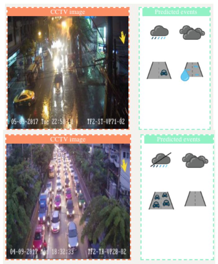
ISPRS Int. J. Geo-Inf. 2019, 8, 128                                                                     2 of 16

closed circuit television (CCTV) is common in many places. CCTV has been deployed in order to
capture images and video of suspicious actions and to provide automatic surveillance in public
spaces. The common goals of such systems include crime prevention and detection by tracking
and observation.
      In Bangkok, the number of CCTV cameras has dramatically increased over the past few years,
relative to other sensors. CCTV has been widely adopted for surveillance in community areas and
real-time monitoring of traffic. Almost 50,000 cameras have been installed in the city [3]. The Bangkok
Metropolitan Administration (BMA) has the responsibility of managing these cameras. They developed
real-time services for groups who require access to real-time traffic monitoring through the BMA
traffic website. Monitoring the increasing number of CCTVs is challenging and requires many
operators. An automated system is one solution that can reduce the workload of operators. Therefore,
to obtain useful information from CCTV images, many researchers have proposed applications for
analyzing them.
      Many automated systems for CCTV surveillance and traffic monitoring have emerged in recent
years, especially in the field of transportation: e.g., traffic surveillance [4], vehicle counting, recognition
and identification, lane detection, and traffic sign detection [5]. However, there is little research
focusing on road environments that can extract weather information [6]. Road conditions affect road
safety, and bad conditions often result in low visibility, such that drivers should be warned or made
aware of the conditions of the road. Several algorithms that can analyze both CCTV video and images
have been proposed. Indeed, due to the complexity of CCTV images, ample information can be
identified in each scene. For example, it can be determined that it is raining, that the road is wet,
and that it is dark. Figure 1 shows a CCTV image of different events in one scene: raining, crowded
traffic, and wet road conditions.

               Figure 1. CCTV scene showing various events: raining, crowded traffic, and wet roads.

     To deal with multiple concurrent events in image scenes, multi-label classification is used to predict
several labels at once. The preparation process is also less time-consuming than other techniques,
such as detection and segmentation, which require several bounding boxes and masking objects
for training. Machine learning techniques have been proposed for multi-label problems, such as
supervised and unsupervised classification, as well as a support vector machine (SVM) classifier
with label relation benchmarking on different datasets [7], which is an example of a supervised task.
Another type of machine learning is deep learning, which has been adopted widely in many fields
due to its hardware capabilities and relatively low GPU cost. In terms of accuracy, deep learning
outperforms other methods.
     Deep learning techniques have become state-of-the-art for classification [8–12], object
detection [13–16], and segmentation tasks [17–20]. Additionally, one of these techniques,
the convolutional neural network, is well known and performs well in image recognition. Numerous
architectures have been offered in order to operate with several applications and datasets. For instance,
VGG [8], GoogleNet [9], and ResNet [10] are stacked with many hidden layers, such as convolutional
layers, max pooling layers, and fully-connected layers. The purpose of adding together these layers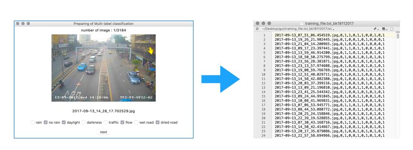
ISPRS Int. J. Geo-Inf. 2019, 8, 128                                                               3 of 16

on top is to increase accuracy. However, too many layers lead to increased training and prediction
time. Therefore, to implement real-world data practically, such as data from CCTV image sequences,
prediction time is of significant concern.
     The contributions of this research are as follows:

•     We extract a combination of road environment situations, such as rain, no rain, daylight,
      darkness, crowded traffic, non-crowded traffic, wet roads, and dry roads, by using a multi-label
      convolutional neural network with existing CCTV images—eliminating the need for new sensors
      designed specifically for such tasks, reducing costs—and detect multiple events at the same time.
•     The developed network has only a few convolutional layers, with the addition of dropout and
      batch normalization layers. The network performed well on our multi-label dataset in terms
      of performance and efficiency. We compared it to other models, such as VGG and ResNet,
      which provide high performance, but require a high amount of computational time for processing.
•     Finally, we propose an application framework to test our model, and we expect that it can be
      implemented in many different locations, including developing countries, which have a large
      number of CCTV images but lack specific sensors. To our knowledge, no other framework
      has been proposed that uses CCTV images to extract the road environment with a multi-label
      classification technique.

2. Related Works

2.1. CCTV and Road Environment Applications
     Other public image data sources, such as Flickr, have been utilized to obtain the geo-tagged
information of each image. For example, [21] used Flickr to develop a recommendation system
for tourist locations using collaborative filtering and context ranking. Additionally, [22] proposed
geolocation-based image retrieval to identify geolocations using visual attention and color descriptors.
In terms of our research, however, CCTVs publicly provide real-time visual and geolocation
information based on the CCTV’s location, unlike Flickr and other data sources.
     Due to the benefits and availability of CCTV, the number of related applications has been
increasing. Most have been applied for surveillance and transportation purposes. Grega et al. [23]
proposed automated detection and recognition of harmful situations by using visual descriptors with
SVM techniques to detect firearms. Additionally, [24] developed 3D convolutional neural networks
in order to recognize human actions by applying 3D convolutions to extract features from spatial
and temporal dimensions and compared the model with a public dataset. However, this technique
requires high computational time and hardware capacity. Similarly, a human action-detection
technique with a traditional hand-engineered feature called MoSIFTwas proposed [25]. In terms
of transportation, CCTV video and images have mostly been used for traffic control applications
by extracting information from the images, such as speed, traffic composition, traffic congestion,
vehicle shapes, vehicle types, vehicle identification numbers, and the occurrence of traffic violations
or road accidents [26–29]. Indeed, insufficient research has taken advantage of CCTV to extract
weather information. Road surface conditions such as slippery roads and dry roads have not been
well examined. To our knowledge, all such research focuses on individual problems for both weather
information and road surface conditions. Rather, they should be connected together insofar as they
relate to road safety. Lee et al. [6] used Korean CCTV video data to extract weather information by
finding video data patterns, calculating similarity scores and constructing a decision tree to predict
sunny, cloudy, and rainy weather. Another example used deep learning techniques with existing CCTV
cameras to detect sea fog automatically [30].

2.2. Multi-Label Classification
    To extract several conditions from a single-image scene at once, multi-label classification
has been introduced. Cheng et al. [17] proposed a recent framework for MsDPD-based feature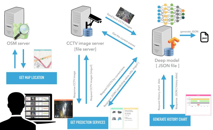
ISPRS Int. J. Geo-Inf. 2019, 8, 128                                                                 4 of 16

representation with a new objective function by solving the problem of multiple variations in a
multi-label classification task, using the PASCAL dataset. The framework outperformed other models
in terms of accuracy, but the technique is still difficult to train end-to-end due to the objective
function. Maxwell et al. [31] presented health-risk prediction for multi-label problems with respect to
chronic diseases. Their evaluation revealed more accuracy than traditional classification techniques
such as decision trees, sequential minimal optimization, and multi-layer perception. Moreover,
Zhuang et al. [32] developed their own network, combining three sub-networks and applying transfer
learning techniques to classify 40 facial attributes. The network is able to detect facial expressions and
hair color, for instance. Their proposed networks outperformed others in terms of accuracy. Not only
did the images work with multi-label problems, but other data, such as text and audio, could also be
classified [33,34]. Finally, the work in [35] developed a model for automatic tag recommendation in a
social bookmark system using a simple binary relevance (BR) algorithm evaluated by the F-measure.
     Our proposed system is based on a combination of weather information, road surface conditions,
and road traffic monitoring, including crowded and non-crowded traffic, by utilizing multi-label
classification with convolutional neural networks to extract useful information from CCTV images.

3. Materials and Methods
     Initially, our system was divided into three main parts. We prepared the dataset by assigning
a one-hot label of each event to each image, and we developed an optimum model for multi-label
classification to identify four pairs of events: raining and not raining, daylight and darkness, crowded
and non-crowded traffic, and wet and dry road surfaces. We then developed this optimum model
and evaluated it. To experiment in real situations, the system was combined with two parts. We first
prepared classifying services to interpret image sequences as predicted events. To generate the
data-interchange JSON format, a road environment monitoring website was then implemented to
evaluate our framework. Further details are provided in each section below.

3.1. Dataset
      In Bangkok, CCTV systems are divided into two types based on whether they are used to monitor
traffic manually or for surveillance. The traffic-monitoring CCTVs are publicly available on the BMA
website, which means that anyone can access them to monitor traffic. The CCTV images are not stored,
however. The second type of CCTV system is for surveillance purposes. Its images are recorded,
but the public does not have access to the data owing to privacy concerns. BMA staff are granted
access only when there is an anomaly or a crime, and the system is then mostly used for investigative
purposes. In our study, we used traffic-monitoring CCTVs. We developed a script to capture images
every 5 s from the BMA website between 1 September 2017 and 10 September 2017 (10 days) from 5
cameras placed in different areas. There were eight categories of concern: raining, not rain, daylight,
darkness, crowded traffic, non-crowded traffic (flow traffic), wet road, and dry road. The definition of
each class is given in Table 1, and examples are shown in Figure 2.
      Each image was manually assigned with multi-label classes by representing the one-hot encoder.
If the image has an event class such as raining, it is assigned 1; if no event occurs, it is assigned 0.
Examples of assigning multiple events are shown in Figure 3. The image on the left was assigned
the one-hot encoder as follows: (0,1,0,1,0,1,0,1). This represents the following: non-rain, darkness,
flow traffic, and dry road. Assigning one-hot multi-label classes is difficult, because there is no
software available for doing so. Thus, we developed a Python GUI script to assign multi-label
events easily for each image, as shown in Figure 4. The script consecutively reads all images in the
training directory. Each label was manually checked by users following the events occurring in the
images until all images were read. Ultimately, a CSV file was generated automatically, containing
the information about each image, including the image name and the assigned one-hot encoders.
This information is freely available on GitHub [36]. The dataset was then split into three groups,
for training, validation, and testing. Due to limited hardware capacity—namely, a GPU GeForce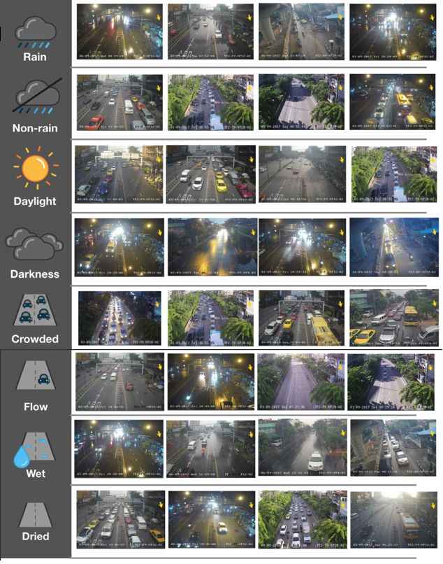
ISPRS Int. J. Geo-Inf. 2019, 8, 128                                                                                   5 of 16

GTX 1070—the number of training datasets was constrained. Images were randomly selected and
unduplicated for the three groups: 4000, 1600, and 1600 images, for training, validation, and testing,
respectively. Each class was given at least 500 images for the training set and 200 for the validation and
testing sets. The validation set was evaluated and used during training to tune the hyperparameters of
the deep model. Additionally, the test set was used after the model was trained in order to calculate
evaluation metrics, including the Hamming loss, mean average precision, and exact match accuracy.

                                          Table 1. Class definition of the dataset.

         Class                        Definition
         Rain                         There are droplets or rain streaks, or the image is blurry due to heavy rain.
         Non-rain                     There are no components of rain in the image.
         Daylight                     Sunlight is evident during the day, normally from 7:00–17:00.
         Darkness                     There is darkness because it is night or because of a lack of sunlight
                                      during the day.
         Crowded traffic              An image is equally divided into four parts. If there are groups of cars in
                                      all four parts, we define the image as showing crowded traffic.
         Flow traffic                 If there are no cars in any of the four areas, the scene is considered to
                                      show flow traffic.
         Wet road                     The road appears to have water on the surface.
         Dry road                     The road does not appear to have water on the surface.

                                       Figure 2. Examples of images for each class.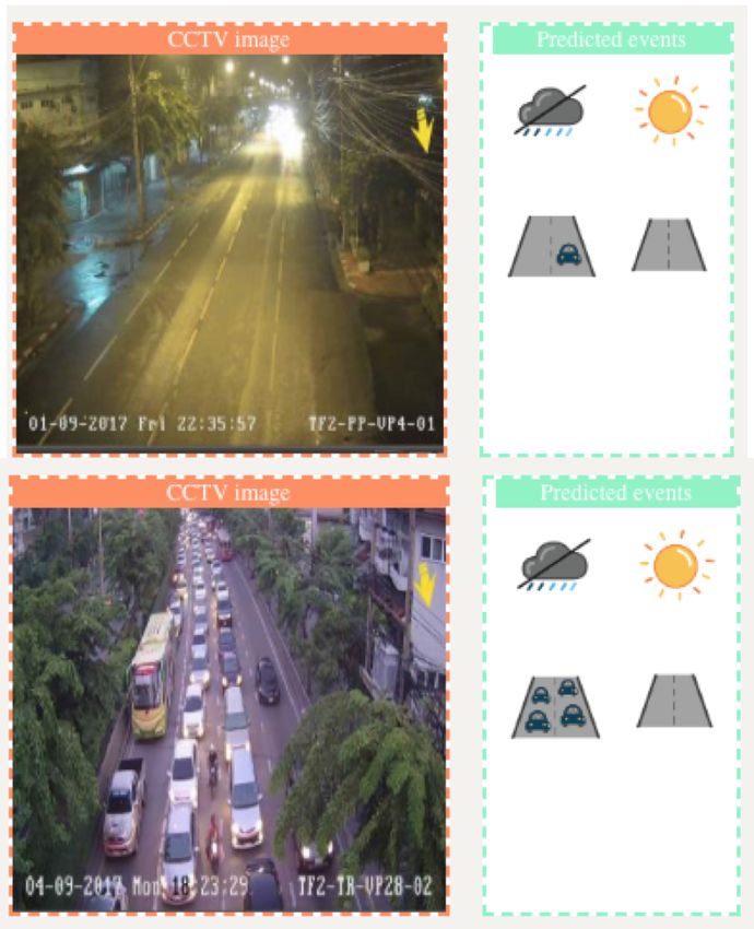
ISPRS Int. J. Geo-Inf. 2019, 8, 128                                                                              6 of 16

                     Figure 3. Example of multiple events in images represented as one-hot labels.

                                      Figure 4. Assigning the one-hot label to each image.

3.2. Model
     In our study, we focus on the convolutional neural network (CNN). CNNs have become well
known for image recognition and classification, due to their automatic feature extraction techniques,
unlike traditional hand-crafted feature techniques such as HOG [37] and SIFT [38]. We experimented
with and developed the CNN model, and we used transfer learning techniques with VGG and ResNet
and the six models we developed in our study.
     First, pre-processing involved resizing the image to 224 × 224 pixels using bicubic interpolation
from OpenCV to compare transfer learning with the VGG and ResNet models. The input size must be
the same in each case. All models were set with the configuration shown in Table 2.

                                             Table 2. Configuration for all models.

  Input Size                    Optimizer                 Learning Rate    Batch Size   Epochs       Loss Function
   224 × 224      Stochastic gradient descent (SGD)           0.0001           12            40   Binary cross-entropy

      The first and second models were trained using transfer learning techniques, VGG16 and
VGG19 [8]. ImageNet [39] weights were applied. There were 10 frozen low-level layers, and the
last dense layer was changed from 1000 to 8, to refer the ImageNet class to our dataset classes. We also
modified the last activation from softmax to sigmoid. We applied the eighth model—the ResNet
model—in a similar manner. However, with ResNet, we did not freeze any layers. The network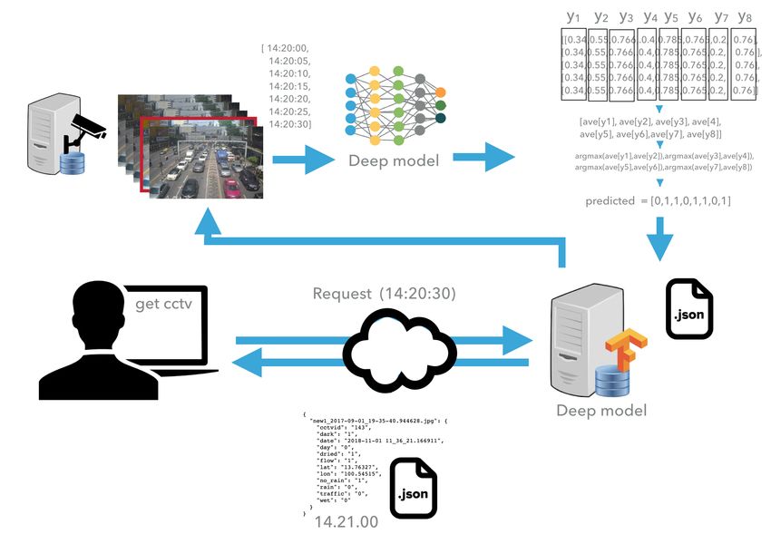
ISPRS Int. J. Geo-Inf. 2019, 8, 128                                                                    7 of 16

was then trained using SGD, as described in Table 2. The softmax function is normally applied for
multi-class classification with a single label, and the classified result is typically assigned a set of
predicted labels, containing eight elements represented by each class. In our case, however, binary
classification with sigmoid was considered. The sigmoid function is defined in Equation (1). Finally,
a ninth model was designed to test how many classes should be selected and whether merging classes
affects the overall accuracy. The model applied the same architecture as the fifth model, but it was
trained differently, by grouping the eight classes into the four following opposite-pair events: rain and
non-rain, daylight and night-time, crowded and flow traffic, and wet and dry road. The positive classes
were trained with rain, daylight, traffic, and wet road. The remaining were considered negative classes.

                                                           1
                                              f (x) =                                                     (1)
                                                        1 + e− x
where x can be interpreted as a probability, if x −         → −∞; f ( x ) −
                                                                          → 0 and when x − → +∞; f ( x ) −
                                                                                                         → 1.
Therefore, the output value ranges from 0–1. For example, if the image is calculated as a set of
predicted labels {0.7, 0.3, 0.3, 0.6, 0.2, 0.7, 0.8, 0.3}, the image has an acceptable probability of showing
rain, darkness, flow traffic, and wet road. To evaluate the model in terms of, for instance, exact match
accuracy, we translated those events from the probabilistic value by defining the threshold value at 0.5,
similar to [31]:                                        (
                                                            0, y < 0.5
                                               f (y) =                                                     (2)
                                                            1, y ≥ 0.5

where y is a predicted value from the sigmoid function. If y is equal to or greater than 0.5, it is assigned
1; otherwise, it is 0, which implies this event is not in the image. In the case of the ninth model, if y is
equal to or greater than 0.5, 1 will be assigned as a positive class, and the opposite class is automatically
assigned 0. Conversely, if y is lower than 0.5, 1 will be assigned a negative class, and 0 will be assigned
to the opposite class.
      The third model differed from the previous models. This model was developed from scratch.
We attempted to reduce the number of layers—and hence the training and prediction time—while
retaining sufficient accuracy. The model was stacked up with fewer layers compared to the VGG
and ResNet architectures. There were thus four convolutional layers with a filtering of 32, 32, 64,
and 64, consecutively. ReLU activation and max pooling layers were later added, with the same
configurations. This model was based on the architecture of the fourth, fifth, sixth, seventh, and ninth
models. The architectures of these models are shown in Table 3. For the fourth model, we added
three dropout layers. Normally, dropout layers are added before the fully-connected layer [40],
which was tested in the seventh model. The work in [41] has shown that dropout layers can be added
to convolutional layers, as well, so we experimented with both cases in the fifth and seventh models.
To prevent overfitting of the model, regularization techniques were used. The dropout is often applied
to deep neural networks. The idea is to temporarily and randomly drop some neurons out of the
hidden or visible layers. The dropout rate indicates how many units must be dropped. When selecting
the dropout rate, we were concerned that the models did not have many parameters related to the early
layers in the convolutions, and therefore, we set a dropout rate of only 0.25. The last fully-connected
layer was then set to 0.5. Moreover, for the fifth architecture, we removed a convolutional layer with
32 filters and added a batch normalization (BN) layer [42]. To improve network stability, the output of
the activation layers can be normalized by the batch mean, which needs to be subtracted and divided
by the batch standard deviation. We applied BN before the last ReLU activation function. For the sixth
model, we pulled out one more 64-filter convolutional layer and kept everything else identical to the
fifth model. All models were evaluated by considering the accuracy of the predicted results and also
according to the time required for training and predicting images.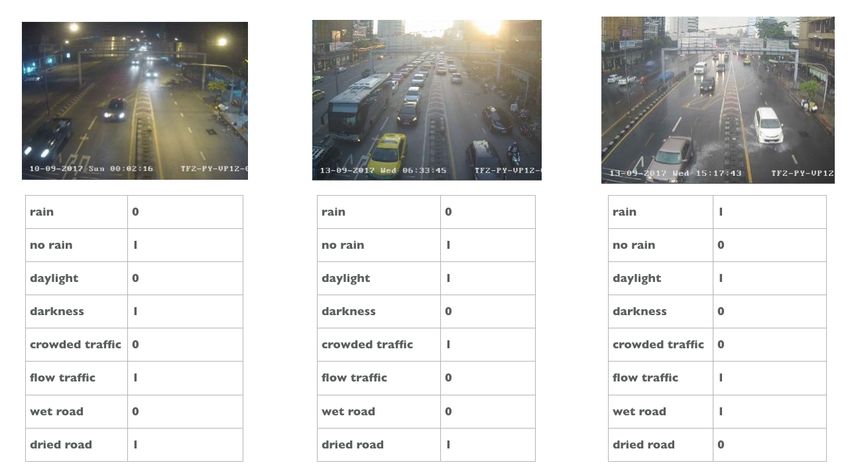
ISPRS Int. J. Geo-Inf. 2019, 8, 128                                                                              8 of 16

                   Table 3. Architecture of the third, fourth, fifth, sixth, seventh, and ninth models.

    No.     Third              Fourth            Fifth            Sixth             Seventh          Ninth
    1       Conv 32            Conv 32           Conv 32          Conv 32           Conv 32          Conv 32
    2       ReLU               ReLU              ReLU             ReLU              ReLU             ReLU
    3       Conv 32            Conv 32           -                -                 -                -
    4       ReLU               ReLU              -                -                 -                -
    5       Max pooling        Max pooling       Max pooling      Max pooling       Max pooling      Max pooling
    6       -                  Dropout(0.25)     Dropout(0.25)    Dropout(0.25)     -                Dropout(0.25)
    7       Conv 64            Conv 64           Conv 64          Conv 64           Conv 64          Conv 64
    8       ReLU               ReLU              ReLU             ReLU              ReLU             ReLU
    9       Conv 64            Conv 64           Conv 64          -                 Conv 64          Conv 64
    10      ReLU               ReLU              ReLU             -                 ReLU             ReLU
    11      Max pooling        Max pooling       Max pooling      Max pooling       Max pooling      Max pooling
    12      -                  Dropout(0.25)     Dropout(0.25)    Dropout(0.25)     Dropout(0.25)    Dropout(0.25)
    13      Flatten            Flatten           Flatten          Flatten           Flatten          Flatten
    14      Dense 512          Dense 512         Dense 512        Dense 512         Dense 512        Dense 512
    15      -                  -                 BN               BN                BN               BN
    16      ReLU               ReLU              ReLU             ReLU              ReLU             ReLU
    17      -                  Dropout(0.5)      Dropout(0.5)     Dropout(0.5)      Dropout(0.5)     Dropout(0.5)
    18      Dense 8            Dense 8           Dense 8          Dense 8           Dense 8          Dense 4
    19      Sigmoid            Sigmoid           Sigmoid          Sigmoid           Sigmoid          Sigmoid
            15 layers          18 layers         17 layers        15 layers         16 layers        17 layers

3.3. System Architecture
     The model was selected following the performance and efficiency criteria that are described below.
To implement the system and to experiment practically with how a selected model works with the
BMA dataset, the model was plugged into the system, as shown in Figure 5.

                                           Figure 5. Overall system architecture.

     Our developed architecture comprises different parts. The first part finds the optimum model
for the dataset, as described above. The second part develops the prediction service to classify the
image into related events. This service was developed using Flask. The input receives the current
time from the clients, and the model server then processes by querying the image sequences with the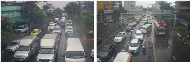
ISPRS Int. J. Geo-Inf. 2019, 8, 128                                                               9 of 16

specific time period from the CCTV server and feeds that to the model in order to predict the road
conditions. To deal with fluctuating images—which sometimes come from CCTV-generated images,
manifesting in the form of features such as blanks, frozen images, and images in black and white—and
in order to improve the accuracy of the model, the system calculates the average probability value of
each predicted event from the specific period of time, as follows:

                                                              n
                                                         1
                                                  AE =
                                                         n   ∑ P ( x ).                              (3)
                                                             i =1

where x is the predicted probability value of each event from the sigmoid function in Equation (1)
and n is expressed as the number of images at a specific period of time. Normally, the period of
time will be set to one minute. AE is denoted as the average of x. In the case of independently
operating eight classes in the practical implementation, it is insufficient to define the probability of
possible events by thresholding via Equation (2), owing to conflicting events such as rain and non-rain
occurring at the same time, which occur less frequently due to our model’s performance. Such events
are identified as opposite-pair events, which contain a set of probabilities of possible and opposite
events. We apply the argmax function to opposite-pair events and define the threshold as Equation (4);
however, for independent events, we still follow Equation (2).

                                             C = argmax ( AEp , AEo ).                               (4)

where C is the value of the argmax, which is an index value of the possible event (p). The possible
event will be set to 1, and the other elements in the opposite-pair events will be set to 0, indicating
opposite events (o). The server dynamically responds to the clients with a one-hot label in JSON
format, as shown in Figure 6. The JSON is contained with a set of information consisting of the image
name, camera number, date and time, and a set of predicted one-hot label.

                                      Figure 6. Process of predicting the service.
ISPRS Int. J. Geo-Inf. 2019, 8, 128 10 of 16
4. Results and Discussion
4.1. Evaluation Metrics
During training, the model calculates the validation dataset using the binary cross-entropy loss
with 40 epochs, as shown in Figure 7. This was insufficient for examining this model in terms of
whether it performed well or not. Other evaluation techniques are required. According to the line
chart, the loss of the third model fluctuated and increased during the training process and did not
substantially decrease during the last epoch. Conversely, the first and second models performed quite
well. The loss continuously declined to 0.157 at the end. On the other hand, the loss of the fifth, sixth,
seventh, and ninth models reached 0.115, 0.113, 0.122, and 0.122 at the end, respectively, and these
models applied the dropout and batch normalization techniques. There were some layers that were
pulled out from the network. Finally, the loss of the eighth model decreased to 0.149, which was tested
on ResNet. Regarding the multi-label classification problem, the model could not be selected using
only this evaluation.
Figure 7. Validation loss during training for 40 epochs.
To evaluate the performance and efficiency of each model, different types of evaluation methods
were taken into account. Additionally, we employed a test dataset to evaluate our result. This dataset
contained 1600 images and constituted around 40% of the training dataset. Common tasks such as
binary and multi-class classification were predicted as a single label. The traditional evaluation metrics,
such as precision, recall, and F-score, can be calculated to define the degree of accuracy with which
the model can perform, while the multi-label problem deals with a set of predicted labels. However,
these evaluation methods are insufficient to define the performance of the model, because the set
of predicted labels can only be considered fully correct, partially correct, or fully wrong. Therefore,
to evaluate the multi-label problem, we needed additional metrics such as the Hamming loss, subset
accuracy (exact match ratio), and average precision [33,34].
The Hamming loss was measured by how many times on average incorrect labels were predicted.
Expecting the value to be close to zero, a lower value means less error, as shown in Equation (5),ISPRS Int. J. Geo-Inf. 2019, 8, 128 11 of 16
where ∆ denotes the difference between Y (the real value) and Z (the predicted one), k represents the
number of classes (eight, in this case), and n is the number of predicted samples:
11 n
n k i∑
Hammingloss( HL) = | Yi ∆Zi | (5)
=1
The exact match ratio (sometimes referred to as the subset accuracy [33]) normally measures the
set of predicted labels against the set of true labels, considering only that both sets must be exactly
the same, meaning that both are fully correct. However, this evaluation method cannot examine the
partial correctness of a set of predicted labels. The equation is as follows:
n
1
ExactMatchRatio =
n ∑ [[Yi = Zi ]]. (6)
i =1
To investigate our model precisely—i.e., to determine whether each class is well predicted,
and which classes perform better than other classes—the average precision (AP) needs to be calculated.
AP can be computed by finding the average over precision and recall. In our experiment, the AP was
calculated using the scikit-learn library [43]. Finally, in order to compare all the models, the mean
average precision (MAP) was calculated by finding the mean of the AP of each class, as shown in
Equation (7). The calculated AP values of our experiments are shown in Table 4. The Hamming loss
and exact match ratio are shown in Table 5. The training and testing times were compared. They were
measured against 4000 images for the training time and 1600 images for the prediction time.
1 k
k i∑
MAP = AP(i) . (7)
=1
Table 4. Average precision of each class.
Model Rain No-Rain Daylight Nighttime Crowded Flow Wet Dried MAP
1st 0.920 0.972 0.969 0.956 0.843 0.888 0.916 0.974 0.930
2nd 0.885 0.992 0.977 0.955 0.879 0.847 0.893 0.989 0.927
3rd 0.909 0.982 0.981 0.938 0.797 0.899 0.942 0.980 0.928
4th 0.892 0.987 0.985 0.959 0.813 0.924 0.935 0.980 0.934
5th 0.942 0.986 0.984 0.967 0.839 0.935 0.966 0.989 0.951
6th 0.940 0.987 0.993 0.940 0.831 0.921 0.977 0.982 0.946
7th 0.949 0.989 0.990 0.947 0.823 0.931 0.970 0.986 0.948
8th 0.925 0.976 0.967 0.966 0.831 0.909 0.959 0.938 0.938
9th 0.945 0.971 0.986 0.951 0.834 0.921 0.963 0.972 0.942
Table 5. Hamming loss, exact match ratio, and training and prediction times.
Model Exact Match Hamming Loss MAP Training Time (minutes) Prediction Time (seconds)
1st 0.763 0.05 0.93 00:31 00:00:22
2nd 0.760 0.060 0.927 00:38 00:00:25
3rd 0.775 0.055 0.928 00:28 00:00:09
4th 0.792 0.051 0.942 00:29 00:00:10
5th 0.84 0.039 0.951 00:23 00:00:09
6th 0.831 0.042 0.946 00:23 00:00:09
7th 0.832 0.043 0.948 00:23 00:00:09
8th 0.776 0.053 0.938 00:55 00:00:33
9th 0.84 0.045 0.942 00:24 00:00:09ISPRS Int. J. Geo-Inf. 2019, 8, 128 12 of 16
We selected the optimum model based on the following results from the evaluation metrics.
The first, second, and eighth models showed lower performance; however, we trained them by
freezing some of the layers without any additional layers from the original VGG and ResNet
models. We assumed that if the networks were added up and fine-tuned, such as the dropout layers,
the accuracy would improve. Regarding the limitation of our hardware and practical implementation
with a near-real-time system, the training and prediction times were crucial. Therefore, selecting
these VGG and ResNet models would be inappropriate in this case. Additionally, the third model
showed the lowest score in terms of exact match accuracy without any additional dropout or BN layers.
Conversely, its prediction time was acceptable for the road environment system. Therefore, the third
model was selected as a base model, and we attempted to fine-tune this model to achieve better
accuracy with the same prediction time. We created the fourth model by adding three dropout layers,
which slightly increased the accuracy. The BN techniques were added in the fifth, sixth, and seventh
models, and we also reduced some unnecessary convolutional layers due to a reduced prediction time.
The performance of the exact match accuracy improved to 10%. Moreover, two convolutional layers
were removed in the sixth model, and the time and accuracy did not change; however, the Hamming
loss was increasing with respect to the previous model. The fifth and seventh models were not
much different in terms of the exact match ratio when the dropout layer was removed before the
convolutional layer, but the fifth model still performed well in terms of the Hamming loss and MAP,
indicating that adding dropout layers before convolutional layers slightly improved the accuracy.
Moreover, the comparison between training the eight classes individually and grouping four positive
and four negative classes is provided for the fifth and ninth models, respectively. They did not
change significant, but the Hamming loss and MAP were slightly different. Training the eight classes
individually performed slightly better. Further, the AV of negative classes was insignificant with the
fifth model. For the purpose of implementation, both cases were appropriately concerned, depending
on dataset availability. The fifth model was selected as the implementation model for our purposes in
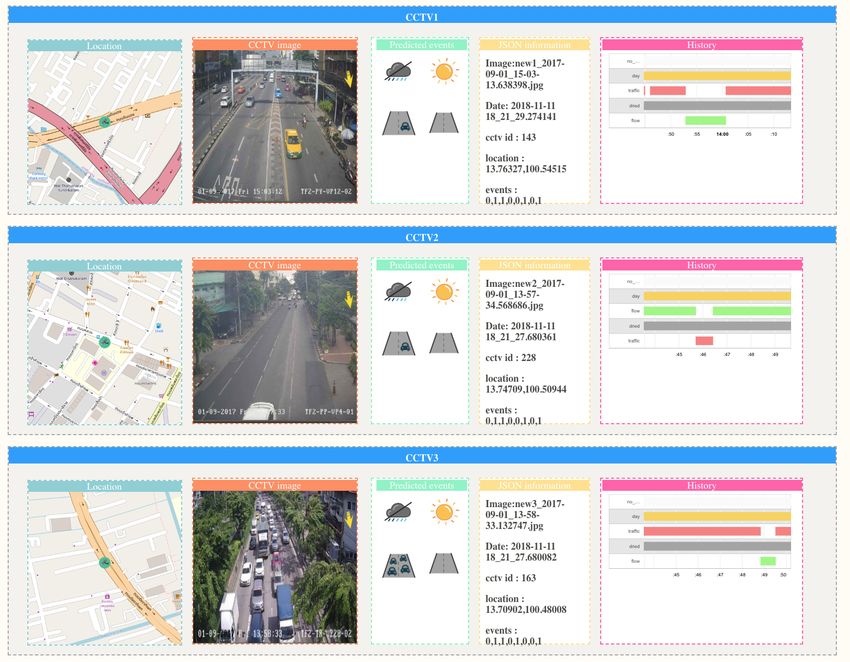
terms of overall performance and efficiency. Examples of predicted results from the selected model are
shown in Figure 8. Figure 8a shows the total correct classification results of the images; conversely,
Figure 8b shows what is partially correct. The darkness scene in the top image was misclassified
as daylight. The bottom image was taken at night; however, the model classified it as daylight,
which differed from the correct one in the bottom image in Figure 8a.
(a) Correct classification (b) Misclassification
Figure 8. Examples of correct and incorrect classifications.
4.2. Road Environment Extraction System
A prototype for a website was developed in order to test our proposed framework. The design
of the system is shown in Figure 9; there are different parts to the system. The first part shows theISPRS Int. J. Geo-Inf. 2019, 8, 128 13 of 16
location of the CCTV cameras after a request from Open Street Map (OSM). The second part shows the
CCTV image sequences, which change dynamically each minute. The third panel represents predicted
values from the JSON response, with intuitive icons. If the predicted results are returned as 1, an event
has occurred, and the relevant icon will appear. The yellow box is displayed as JSON text containing
the CCTV information. The last panel shows the timeline of each event, representing an entire day.
For this experiment, we used only five CCTV cameras. An example of the results is shown in a video
available on YouTube [44].
Figure 9. Prototype of the road environment extraction system.
5. Conclusions and Outlooks
Insofar as existing CCTV cameras can be utilized to extract road environment information such
as weather data, traffic, and road surface conditions, all of which are vital to drivers, we proposed
a framework to extract this information by applying multi-label CNN classification with a BMA
dataset. Different models, including state-of-the-art models such as VGG and ResNet, were compared
to our customized model. We trained individual classes and grouped positive and negative classes.
Our results indicated that the former strategy performed slightly better, although grouping opposite
classes was less time consuming when preparing the dataset. Additionally, evaluation indices such as
the Hamming loss, exact match accuracy, and MAP were measured in addition to the training and
prediction times. Our model performed well in terms of accuracy and time consumption, with few
convolutional layers as a result of adding dropout and BN layers. Additionally, a prototype for our
system was developed to demonstrate the feasibility of the model in terms of analyzing CCTV images.
Future work will entail creating more classes and further generalizing the model, such that the system
can be utilized with various types of CCTV systems in developing countries. We will also explore the
extraction of road patterns using time series analysis.ISPRS Int. J. Geo-Inf. 2019, 8, 128 14 of 16
6. Software and Hardware to Be Used
The software used in our study to prepare labels and assign them to the datasets and models
was developed with Python using the Keras library, with the Tensorflow backend and the scikit-learn
library. Images were preprocessed using OpenCV 3.3. Web services were generated with the Flask
library. Additionally, the front-end website for testing our experiment was developed using HTML,
JavaScript, and the jquery framework. In addition, we used an Xeon 2.4-GHz CPU with GeForce
GTX 1070.
Author Contributions: Chairath Sirirattanapol proposed and developed the methodology, designed the
experiment of the study, and conducted all experiments. Masahiko NAGAI and Apichon Witayangkurn
were direct advisors, providing useful recommendations about deep learning algorithms and performance
improvements. Surachet Pravinvongvuth provided guidance related to transportation and advice about the
source of the datasets. Mongkol Ekpanyapong recommended the BMA dataset with related image processing
techniques.
Funding: This research received no external funding.
Acknowledgments: This work could not have been successfully realized without the assistance of the Bangkok
Metropolitan Administration (BMA), and all BMA staff who assisted in collecting the data.
Conflicts of Interest: The authors declare no conflict of interests
Abbreviations
The following abbreviations are used in this manuscript:
AP Average precision
BMA Bangkok Metropolitan Administration
BN Batch normalization
CCTV Closed circuit television
CNNs Convolutional neural networks
GPU Graphics processing unit
JSON JavaScript Object Notation
MAP Mean average precision
OSM Open Street Map
ReLU Rectified linear unit
SGD Stochastic gradient decent
SVM Support vector machine
References
1. Goodwin, L.C. Weather Impacts on Arterial Traffic Flow; Mitretek Systems Inc.: Falls Church, VA, USA, 2002.
2. Haug, A.; Grosanic, S. Usage of road weather sensors for automatic traffic control on motorways.
Transp. Res. Procedia 2016, 15, 537–547. [CrossRef]
3. Trimek, J. Public confidence in CCTV and Fear of Crime in Bangkok, Thailand. Int. J. Crim. Justice Sci. 2016,
11, 17.
4. Nemade, B. Automatic traffic surveillance using video tracking. Procedia Comput. Sci. 2016, 79, 402–409.
[CrossRef]
5. Mogelmose, A.; Trivedi, M.M.; Moeslund, T.B. Vision-Based Traffic Sign Detection and Analysis for Intelligent
Driver Assistance Systems: Perspectives and Survey. IEEE Trans. Intell. Transp. Syst. 2012, 13, 1484–1497.
[CrossRef]
6. Lee, J.; Hong, B.; Shin, Y.; Jang, Y.J. Extraction of weather information on road using CCTV video.
In Proceedings of the 2016 International Conference on Big Data and Smart Computing (BigComp), Hong
Kong, China, 18–20 January 2016.
7. Fu, D.; Zhou, B.; Hu, J. Improving SVM based multi-label classification by using label relationship.
In Proceedings of the 2015 International Joint Conference on Neural Networks (IJCNN), Killarney, Ireland,
12–17 July 2015.ISPRS Int. J. Geo-Inf. 2019, 8, 128 15 of 16
8. Simonyan, K.; Zisserman, A. Very Deep Convolutional Networks for Large-Scale Image Recognition. arXiv
2014, arXiv:1409.1556.
9. Szegedy, C.; Liu, W.; Jia, Y.; Sermanet, P.; Reed, S.; Anguelov, D.; Erhan, D.; Rabinovich, A. Going deeper
with convolutions. In Proceedings of the IEEE Conference on Computer Vision and Pattern Recognition,
Boston, MA, USA, 7–12 June 2015.
10. He, K.; Zhang, X.; Ren, S.; Sun, J. Deep residual learning for image recognition. In Proceedings of the IEEE
Conference on Computer Vision and Pattern Recognition, Las Vegas, NV, USA, 27–30 June 2016.
11. Xie, S.; Girshick, R.; Dollár, P.; Tu, Z.; He, K. Aggregated residual transformations for deep neural networks.
In Proceedings of the IEEE Conference on Computer Vision and Pattern Recognition , Honolulu, HI, USA,
21–26 July 2017.
12. Cheng, G.; Zhou, P.; Han, J. Duplex metric learning for image set classification. IEEE Trans. Image Process.
2018, 27, 281–292. [CrossRef] [PubMed]
13. Ren, S.; He, K.; Girshick, R.; Sun, J. Faster r-cnn: Towards real-time object detection with region proposal
networks. IEEE Trans. Pattern Anal. Mach. Intell. 2017, 39, 1137–1149. [CrossRef] [PubMed]
14. Liu, W.; Anguelov, D.; Erhan, D.; Szegedy, C.; Reed, S.; Fu, C.Y.; Berg, A.C. Ssd: Single shot multibox detector.
In Computer Vision—ECCV 2016; Springer: Cham, Switzerland, 2016.
15. Redmon, J.; Farhadi, A. Yolov3: An incremental improvement. arXiv 2018, arXiv:1804.02767.
16. Cheng, G.; Han, J.; Zhou, P.; Xu, D. Learning Rotation-Invariant and Fisher Discriminative Convolutional
Neural Networks for Object Detection. IEEE Trans. Image Process. 2019, 28, 265–278. [CrossRef] [PubMed]
17. Cheng, G.; Gao, D.; Liu, Y.; Han, J. Multi-scale and Discriminative Part Detectors Based Features for
Multi-label Image Classification. In Proceedings of the Twenty-Seventh International Joint Conference on
Artificial Intelligence (IJCAI-18), Stockholm, Sweden, 13–19 July 2018.
18. Ronneberger, O.; Fischer, P.; Brox, T. U-net: Convolutional networks for biomedical image segmentation.
In Medical Image Computing and Computer-Assisted Intervention—MICCAI 2015; Springer: Cham,
Switzerland, 2015.
19. Long, J.; Shelhamer, E.; Darrell, T. Fully convolutional networks for semantic segmentation. In Proceedings
of the IEEE Conference on Computer Vision and Pattern Recognition, Boston, MA, USA, 7–12 June 2015.
20. He, K.; Gkioxari, G.; Dollár, P.; Girshick, R. Mask r-cnn. In Proceedings of the 2017 IEEE International
Conference on Computer Vision (ICCV), Venice, Italy, 22–29 October 2017.
21. Memon, I.; Chen, L.; Majid, A.; Lv, M.; Hussain, I.; Chen, G. Travel recommendation using geo-tagged
photos in social media for tourist. Wirel. Pers. Commun. 2015, 80, 1347–1362. [CrossRef]
22. Memon, M.H.; Li, J.P.; Memon, I.; Arain, Q.A. GEO matching regions: Multiple regions of interests using
content based image retrieval based on relative locations. Multimed. Tools Appl. 2017, 76, 15377–15411.
[CrossRef]
23. Grega, M.; Matiolański, A.; Guzik, P.; Leszczuk, M. Automated detection of firearms and knives in a CCTV
image. Sensors 2016, 16, 47. [CrossRef] [PubMed]
24. Ji, S.; Xu, W.; Yang, M.; Yu, K. 3D convolutional neural networks for human action recognition. IEEE Trans.
Pattern Anal. Mach. Intell. 2013, 35, 221–231. [CrossRef] [PubMed]
25. Chen, M.-Y.; Hauptmann, A. Mosift: Recognizing Human Actions in Surveillance Videos. Available online:
http://www.cs.cmu.edu/~mychen/publication/ChenMoSIFTCMU09.pdf (accessed on 30 January 2019).
26. Zhang, W.; Wu, Q.M.J.; Yin, H.B. Moving vehicles detection based on adaptive motion histogram.
Digit. Signal Process. 2010, 20, 793–805. [CrossRef]
27. Kurdi, H.A. Survey on Traffic Control using Closed Circuit Television (CCTV). In Proceedings of the
International Conference on Digital Information Processing, E-Business and Cloud Computing (DIPECC),
Society of Digital Information and Wireless Communication, Dubai, UAE, 23–25 October 2013.
28. Swathy, M.; Nirmala, P.S.; Geethu, P.C. Survey on Vehicle Detection and Tracking Techniques in Video
Surveillance. Int. J. Comput. Appl. 2017, 160, 22–25.
29. Ganesh, R.B.; Appavu, S. An Intelligent Video Surveillance Framework with Big Data Management for
Indian Road Traffic System. Int. J. Comput. Appl. 2015, 123, 12–19.
30. Choi, Y.; Choe, H.G.; Choi, J.Y.; Kim, K.T.; Kim, J.B.; Kim, N.I. Automatic Sea Fog Detection and Estimation
of Visibility Distance on CCTV. J. Coast. Res. 2018, 85, 881–885. [CrossRef]ISPRS Int. J. Geo-Inf. 2019, 8, 128 16 of 16
31. Maxwell, A.; Li, R.; Yang, B.; Weng, H.; Ou, A.; Hong, H.; Zhou, Z.; Gong, P.; Zhang, C. Deep learning
architectures for multi-label classification of intelligent health risk prediction. BMC Bioinform. 2017, 18, 523.
[CrossRef] [PubMed]
32. Zhuang, N.; Yan, Y.; Chen, S.; Wang, H.; Shen, C. Multi-label learning based deep transfer neural network
for facial attribute classification. Pattern Recogn. 2018, 80, 225–240. [CrossRef]
33. Herrera, F.; Charte, F.; Rivera, A.J.; del Jesus, M.J. Multilabel classification. In Multilabel Classification;
Springer: Cham, Switzerland, 2016; pp. 17–31.
34. Sorower, M.S. A literature Survey on Algorithms for Multi-Label Learning; Oregon State University: Corvallis,
OR, USA, 2010; Volume 18.
35. Katakis, I.; Tsoumakas, G.; Vlahavas, I. Multilabel text classification for automated tag suggestion.
In Proceedings of the ECML/PKDD 2008 Discovery Challenge, Antwerp, Belgium, 15–19 September 2008.
36. Available online: https://github.com/chairathAIT/multi-label-assign (accessed on 30 January 2019).
37. Dalal, N.; Triggs, B. Histograms of oriented gradients for human detection. In Proceedings of the IEEE
Computer Society Conference on Computer Vision and Pattern Recognition (CVPR 2005), San Diego, CA,
USA, 20–25 June 2005.
38. Lowe, D.G. Distinctive image features from scale-invariant keypoints. Int. J. Comput. Vis. 2004, 60, 91–110.
[CrossRef]
39. Krizhevsky, A.; Sutskever, I.; Hinton, G.E. Imagenet classification with deep convolutional neural networks.
In Proceedings of the Neural Information Processing Systems (NIPS), Lake Tahoe, NV, USA, 3–6 December
2012; pp. 1097–1105.
40. Srivastava, N.; Hinton, G.; Krizhevsky, A.; Sutskever, I.; Salakhutdinov, R. Dropout: A simple way to prevent
neural networks from overfitting. J. Mach. Learn. Res. 2014, 15, 1929–1958.
41. Park, S.; Kwak, N. Analysis on the dropout effect in convolutional neural networks. In Computer Vision—
ACCV 2016; Springer: Cham, Switzerland, 2016.
42. Ioffe, S.; Szegedy, C. Batch normalization: Accelerating deep network training by reducing internal covariate
shift. arXiv 2015, arXiv:1502.03167.
43. Pedregosa, F.; Varoquaux, G.; Gramfort, A.; Michel, V.; Thirion, B.; Grisel, O.; Blondel, M.; Prettenhofer, P.;
Weiss, R.; Dubourg, V.; et al. Scikit-learn: Machine Learning in Python. JMLR 2011, 12, 2825–2830.
44. Available online: https://www.youtube.com/watch?v=i0FoXhCus4U (accessed on 30 January 2019).
c 2019 by the authors. Licensee MDPI, Basel, Switzerland. This article is an open access
article distributed under the terms and conditions of the Creative Commons Attribution
(CC BY) license (http://creativecommons.org/licenses/by/4.0/).You can also read