Behavior in Strategic Settings: Evidence from a Million Rock-Paper-Scissors Games - MDPI
←
→
Page content transcription
If your browser does not render page correctly, please read the page content below
games
Article
Behavior in Strategic Settings: Evidence from a
Million Rock-Paper-Scissors Games
Dimitris Batzilis 1,† , Sonia Jaffe 2, *,† , Steven Levitt 3,† , John A. List 3,† and Jeffrey Picel 4,†
 1   Department of Economics, American College of Greece—Deree, Agia Paraskevi 15342, Greece;
     dbatzilis@acg.edu
 2   Office of the Chief Economist, Microsoft, Redmond, WA 98052, USA
 3   Department of Economics, University of Chicago, Chicago, IL 60637, USA; slevitt@uchicago.edu (S.L.);
     jlist@uchicago.edu (J.A.L.)
 4   Department of Economics, Harvard University, Cambridge, MA 02138, USA; jpicel@fas.harvard.edu
 *   Correspondence: spj@uchicago.edu
 †   These authors contributed equally to this work.

 Received: 6 February 2019; Accepted: 4 April 2019; Published: 10 April 2019

 Abstract: We make use of data from a Facebook application where hundreds of thousands of people
 played a simultaneous move, zero-sum game—rock-paper-scissors—with varying information to
 analyze whether play in strategic settings is consistent with extant theories. We report three main
 insights. First, we observe that most people employ strategies consistent with Nash, at least some of
 the time. Second, however, players strategically use information on previous play of their opponents,
 a non-Nash equilibrium behavior; they are more likely to do so when the expected payoffs for such
 actions increase. Third, experience matters: players with more experience use information on their
 opponents more effectively than less experienced players, and are more likely to win as a result. We
 also explore the degree to which the deviations from Nash predictions are consistent with various
 non-equilibrium models. We analyze both a level-k framework and an adapted quantal response
 model. The naive version of each these strategies—where players maximize the probability of winning
 without considering the probability of losing—does better than the standard formulation. While one
 set of people use strategies that resemble quantal response, there is another group of people who
 employ strategies that are close to k1 ; for naive strategies the latter group is much larger.

 Keywords: play in strategic settings; large-scale data set; Nash equilibrium; non-equilibrium strategies

 JEL Classification: C72; D03

      Over the last several decades game theory has profoundly altered the social science landscape.
Across economics and its sister sciences, elements of Nash equilibrium are included in nearly every
analysis of behavior in strategic settings. For their part, economists have developed deep theoretical
insights into how people should behave in a variety of important strategic environments—from
optimal actions during wartime to more mundane tasks such as how to choose a parking spot at the
mall. These theoretical predictions of game theory have been tested in lab experiments (e.g., see cites
in [1,2]), and to a lesser extent in the field (e.g., [3–6] and cites therein).
      In this paper, we take a fresh approach to studying strategic behavior outside the lab, exploiting
a unique dataset that allows us to observe play while the information shown to the player changes.

Games 2019, 10, 18; doi:10.3390/g10020018                                       www.mdpi.com/journal/games
Games 2019, 10, 18 2 of 34
In particular, we use data from over one million matches of rock-paper-scissors (RPS) 1 played on a
historically popular Facebook application. Before each match (made up of multiple throws), players
are shown a wealth of data about their opponent’s past history: the percent of past first throws in a
match that were rock, paper, or scissors, the percent of all throws that were rock, paper, or scissors,
and all the throws from the opponents’ most recent five games. These data thus allow us to investigate
whether, and to what extent, players’ strategies incorporate this information.
The informational variation makes the strategy space for the game potentially much larger than a
one-shot RPS game. However, we show that in Nash equilibrium, players must expect their opponents
to mix equally across rock-paper-scissors—same as in the one-shot game. Therefore, a player has no
use for information on her opponent’s history when her opponent is playing Nash.
To the extent that an opponent systematically deviates from Nash; however, knowledge of that
opponent’s history can potentially be exploited.2,3 Yet it is not obvious how one should use the
information provided. Players can use the information to determine whether an opponent’s past play
is consistent with Nash, but without seeing what information an opponent was reacting to (they do not
observe the past histories of the opponent’s previous opponents), it is hard to guess what non-Nash
strategy the opponent may be using. Additionally, players are not shown information about their own
past play, so if a player wants to exploit an opponent’s expected reaction, he must keep track of his
own history of play.
Because of the myriad of possible responses, we start with a reduced-form analysis of the first
throw in each match to describe how players respond to the provided information. We find that players
use information: for example, they are more likely to play rock when their opponent has played more
scissors (which rock beats) or less paper (which beats rock) on previous first throws, though the latter
effect is smaller. When we do the analysis at the player level, 47% of players are reacting to information
about their opponents’ history in a way that is statistically significant.4 Players also have a weak
negative correlation across their own first throws.
This finding motivated us to adopt a structural approach to evaluate the performance of two
well-known alternatives to Nash equilibrium: level-k and quantal response. The level-k model posits
that players are of different types according to the depth of their reasoning about the strategic behavior
of their opponents [15–18]. Players who are k0 do not respond to information available about their
opponent. This can either mean that they play randomly (e.g., [19]) or that they play some focal or
salient strategy (e.g., [20,21]). Players who are k1 respond optimally to a k0 player, which in our context
means responding to the focal strategy of the opponent’s (possibly skewed) historical distribution of
throws; k2 players respond optimally to k1 , etc.5
Level-k theory acknowledges the difficulty of calculating equilibria and of forming equilibrium
beliefs, especially in one-shot games. It has been applied to a variety of laboratory games
(e.g., [19,20,22–24]) and some naturally occurring environments (e.g., [25–29]). This paper has
substantially more data than most other level-k studies, both in number of observations and in
the richness of the information structure. As suggested by an anonymous referee and acknowledged
1 Two players each play rock, paper, or scissors. Rock beats scissors; scissors beats paper; paper beats rock. If they both play
the same, it is a tie. The payoff matrix is in Section 2.
2 If the opponent is not playing Nash, then Nash is no longer a best response. In symmetric zero-sum games such as RPS,
deviating from Nash is costless if the opponent is playing Nash (since all strategies have an expected payoff of zero), but if a
player thinks he knows what non-Nash strategy his opponent is using then there is a profitable deviation from Nash.
3 Work in evolutionary game theory on RPS has looked at how the population’s distribution of strategies evolves towards or
around Nash equilibrium (e.g., [7,8]). Past work on fictitious play has showed that responding to the opponents’ historical
frequency of strategies leads to convergence to Nash equilibrium [9–11]. Young [12] also studies how conventions evolve as
players respond to information about how their opponents have behaved in the past, while Mookherjee and Sopher [13,14]
examine the effect of information on opponents’ history on strategic choices.
4 When doing a test at the player level, we expect about 5% of players to be false positives, so we take these numbers as
evidence on behavior only when they are statistically significant for substantially more than 5% of players.
5 Since the focal k0 strategies can be skewed, our k1 and k2 strategies usually designate a unique throw, which would not be
true if k0 were constrained to be a uniform distribution.Games 2019, 10, 18 3 of 34
in Ho et al. [24], the implication of the fictitious play learning rule is that players should employ a k1
strategy, best responding to the historical frequency of their opponents’ plays on the assumption that
it predicts their future choices. When k1 play is defined as the best response to past historical play, as
in the current context, it is of course indistinguishable from fictitious play.
We adapt level-k theory to our repeated game context. Empirically, we use maximum likelihood
to estimate how often each player plays k0 , k1 , and k2 , assuming that they are restricted to those three
strategies. We find that most of the play is best described as k0 (about 74%). On average, k1 is used in
18.5% of throws. The average k2 estimate is 7.7%, but for only 12% of players do we reject at the 95%
level that they never play k2 . Most players use a mixture of strategies, mainly k0 and k1 .6 We also find
that 20% of players deviate significantly from 13 , 13 , 13 when playing k0 . We also consider a cognitive
hierarchy version of the model and a naive version where players maximize the probability of winning
without worrying about losing. The rates of play of the analogous strategies are similar to the baseline
level-k, but the naive level-k is a better fit for most players.
We also show that play is more likely to be consistent with k1 when the expected return to k1 is
higher. This effect is larger when the opponent has a longer history—that is, when the skewness in
history is less likely to be noise. The fact that players respond to the level of the perceived expected
(k1 ) payoff, not just whether it is the highest payoff, is related to the idea of quantal response: that
players’ probability of using a pure strategy is increasing in the relative perceived expected payoff
of that strategy.7 This can be thought of as a more continuous version of a k1 strategy. Rather than
always playing the strategy with the highest expected payoff as under k1 , the probability of playing a
strategy increases with the expected payoff. As the random error in this (non-equilibrium) quantal
response approaches zero (or the responsiveness of play to the expected payoff goes to infinity) this
converges to the k1 strategy. On average, we find that increasing the expected payoff to a throw by
one standard deviation increases the probability it is played by 7.3 percentage points (more than one
standard deviation). The coefficient is positive and statistically significant for 63% of players.
If players were using the k1 strategy, we would also find that expected payoffs have a positive
effect on probability of play. Similarly, if players used quantal response, many of their throws would
be consistent with k1 and our maximum likelihood analysis would indicate some k1 play. The above
evidence does not allow us to state which model is a better fit for the data. To test whether k1 or
quantal response better explains play, we compare the model likelihoods. The quantal response model
is significantly better than the k1 model for 18.3 percent of players, yet the k1 model is significantly
better for 17.5 percent of players. We interpret this result as suggesting that there are some players
whose strategies are close to k1 , or fictitious play, and a distinct set of players whose strategies resemble
quantal response. We also compare naive level-k to a naive version of the quantal response model.
Here level-k does better. About 12% of players significantly favor the quantal response model and
26% significantly favor the naive level-k. The heterogeneity in player behavior points to the value of
studies such as this one that have sufficient data to do within player analyses. In sum, our data paint
the picture that there is a fair amount of equilibrium play, and when we observe non-Nash play, extant
models have some power to explain the data patterns.
The remainder of the paper is structured as follows. Section 1 describes the Facebook application
in which the game is played and presents summary statistics of the data. Section 2 describes the
theoretical model underlying the game, and the concept and implications of Nash equilibrium in this
setting. Section 3 explores how players respond to the information about their opponents’ histories.
6 As we discuss in Section 4, there are several reasons that may explain why we find lower estimates for k1 and k2 play than
in previous work. Many players may not remember their own history, which is necessary for playing k2 . Also, given that
k0 is what players would most likely play if they were not shown the information (i.e., when they play RPS outside the
application), it may be more salient than in other contexts.
7 Because we think players differ in the extent to which they respond to information and consider expected payoffs, we do
not impose the restriction from quantal response equilibrium theory [30] that the perceived expected payoffs are correct.
Instead, we require that the expected payoffs are calculated based on the history of play. See Section 5 for more detail.Games 2019, 10, 18 4 of 34
Section 4 explains how we adapt level-k theory to this context and provides parameter estimates.
Section 5 adapts a non-equilibrium version of the quantal response model to our setting. Section 6
compares the level-k and quantal response models. Section 7 concludes.
1. Data: Roshambull
RPS, also known as Rochambeau and jan-ken-pon, is said to have originated in the Chinese Han
dynasty, making its way to Europe in the 18th century. To this day, it continues to be played actively
around the world. There is even a world RPS championship sponsored by Yahoo.8
The source of our data is an early Facebook ‘app’ called Roshambull. (The name is a combination
of Rochambeau and the name of the firm sponsoring the app, Red Bull.) Roshambull allowed users to
play RPS against other Facebook users—either by challenging a specific person to a game or by having
the software pair them with an opponent. It was a very popular app for its era with 340,213 users
(≈1.7% of Facebook users in 2007) starting at least one match in the first three months of the game’s
existence. Users played best-two-out-of-three matches for prestige points known as ‘creds’. They could
share their records on their Facebook page and there was a leader board with the top players’ records.
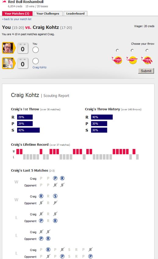
To make things more interesting for players, before each match the app showed them a “scouting
sheet” with information on the opponent’s history of play.9 In particular, the app showed each player
the opponent’s distribution of throws on previous first throws of a match (and the number of matches)
and on all previous throws (and the number of throws), as well as a play-by-play breakdown of the
opponent’s previous five matches. It also shows the opponent’s win-loss records and the number of
creds wagered. Figure 1 shows a sample screenshot from the game.
Our dataset contains 2,636,417 matches, all the matches played between 23 May 2007 (when the
program first became available to users) and 14 August 2007. For each throw, the dataset contains a
player ID, match number, throw number, throw type, and the time and date at which the throw was
made.10 This allows us to create complete player histories at each point in time. Most players play
relatively few matches in our three month window: the median number of matches is 5 and the mean
is 15.11 Figure 2 shows the distribution of the number of matches a player played.
Some of our inference depends upon having many observations per player; for those sections, our
analysis is limited to the 7758 “experienced” players for whom we observe at least 100 clean matches.
They play an average of 192 matches; the median is 148 and the standard deviation is 139.12 Because
these are the most experienced players, their strategies may not be representative; one might expect
more sophisticated strategies in this group relative to the Roshambull population as a whole.
Table 1 summarizes the play and opponents’ histories shown in the first throw of each match,
for both the entire sample and the experienced players. For all the empirical analysis we focus on
the first throw in each match. Modeling non-equilibrium behavior on subsequent throws is more
8 RPS is usually played for low stakes, but sometimes the result carries with it more serious ramifications. During the World
Series of Poker, an annual $500 per person RPS tournament is held, with the winner taking home $25,000. RPS was also
once used to determine which auction house would have the right to sell a $12 million Cezanne painting. Christie’s went
to the 11-year-old twin daughters of an employee, who suggested “scissors” because “Everybody expects you to choose
‘rock’.” Sotheby’s said that they treated it as a game of chance and had no particular strategy for the game, but went with
“paper” [31].
9 Bart Johnston, one of the developers said, “We’ve added this intriguing statistical aspect to the game. . . You’re constantly
trying to out-strategize your opponent” [32].
10 Unfortunately we only have a player id for each player; there is no demographic information or information about their
out-of-game connections to other players.
11 Because of the possibility for players to collude to give one player a good record if the other does not mind having a bad
one, we exclude matches from the small fraction of player-pairs for which one player won an implausibly high share of the
matches (100% of ≥10 games or 80% of ≥20 games). To accurately recreate the information that opponents were shown
when those players played against others, we still include those “collusion” matches when forming the players’ histories.
12 Depending on the opponent’s history, the strategies we look at may not indicate a unique throw (e.g., if rock and paper have
the same expected payoffs); for some analyses we only use players who have 100 clean matches where the strategies being
considered indicate a unique throw, so we use between 5405 and 7758 players.Games 2019, 10, 18 5 of 34
complicated because in addition to their opponent’s history, a player may also respond to the prior
throws in the match.
Figure 1. Screenshot of the Roshambull App.Games 2019, 10, 18 6 of 34
Figure 2. Number of matches played by Roshambull users. Note: The figure shows the number of clean
matches played by the 334,661 players who had at least one clean, completed match (see Footnote 11
for a description of the data cleaning). The data has a very long right tail, so all the players with over
200 matches are grouped together in the right-most bar.
Table 1. Summary Statistics of First Throws.
Full Sample Restricted Sample
Variable
Mean (SD) Mean (SD)
Throw Rock (%) 33.99 (47.37) 32.60 (46.87)
Throw Paper (%) 34.82 (47.64) 34.56 (47.56)
Throw Scissors (%) 31.20 (46.33) 32.84 (46.96)
Player’s Historical %Rock 34.27 (19.13) 32.89 (8.89)
Player’s Historical %Paper 35.14 (18.80) 34.88 (8.97)
Player’s Historical %Scissors 30.59 (17.64) 32.23 (8.57)
Opp’s Historical %Rock 34.27 (19.13) 33.59 (13.71)
Opp’s Historical %Paper 35.14 (18.80) 34.76 (13.46)
Opp’s Historical %Scissors 30.59 (17.64) 31.65 (12.84)
Opp’s Historical Skew 10.42 (18.08) 5.39 (12.43)
Opp’s Historical %Rock (all throws) 35.45 (12.01) 34.81 (8.59)
Opp’s Historical %Paper (all throws) 34.01 (11.74) 34.10 (8.35)
Opp’s Historical %Scissors (all throws) 30.54 (11.07) 31.09 (7.98)
Opp’s Historical Length (matches) 55.92 (122.05) 99.13 (162.16)
Total observations 5,012,128 1,472,319
Note: The Restricted Sample uses data only from 7758 players who play at least 100 matches. The first 3
variables are dummies for when a throw is rock, paper, or scissors (multiplied by 100). The next 3 are the
percentages of a player’s past throws that were each type, using only the first throw in each match. Variables
7–9 are the same as 4–6, but describing the opponent’s history of play instead of the player’s. “All throws” are
the corresponding percentages for all the opponent’s past throws. Opp’s Historical Length is the number of
previous matches the opponent played. Skew measures the extent to which the opponent’s history of first
2
1
throws deviates from random, 100 ∑ %i − 100
3 .
i =r,p,s
2. Model
A standard game of RPS is a simple 3 × 3 zero-sum game. The payoffs are shown in Figure 3.
Its only Nash equilibrium is for players to mix 13 , 13 , 13 across rock, paper, and scissors. Because each
match is won by the first player to win two throws, and players play multiple matches, the strategies
in Roshambull are potentially substantially more complicated: players could condition their play on
various aspects of their own or their opponents’ histories. A strategy would be a mapping from (1)
the match history for the current match so far, (2) one’s own history of all matches played, and (3) the
space of information one might be shown about one’s opponent’s history, onto a distribution of throws.Games 2019, 10, 18 7 of 34
In addition, Roshambull has a matching process operating in the background, in which players from
a large pool are matched into pairs to play a match and then are returned to the pool to be matched
again. In the Appendix A.1, we formalize Roshambull in a repeated game framework.
Player 2:
Rock Paper Scissors
Rock (0,0) (-1,1) (1,-1)
Player 1: Paper (1,-1) (0,0) (-1,1)
Scissors (-1,1) (1,-1) (0,0)
Figure 3. Payoffs for a single throw of rock-paper-scissors.
Despite the potential for complexity, we show the equilibrium strategies are still simple.
Proposition 1. In any Nash equilibrium, for every throw of every match, each player correctly expects his
opponent to mix 13 , 13 , 13 over rock, paper, and scissors.13
Proof. See the Appendix A.1.
The proof shows that since it is a symmetric, zero-sum game, players’ continuation values at
the end of every match must be zero. Therefore, players are only concerned with winning the match,
and not with the effect of their play on their resulting history. We then show that for each throw in
the match, if player A correctly believes that player B is not randomizing 13 , 13 , 13 , then player A has a
profitable deviation.
Same as in the single-shot game, Nash equilibrium implies that players randomize 13 , 13 , 13 both
unconditionally and conditional on any information available to their opponent. Out of equilibrium,
players may condition their throws on their or their opponents’ histories in a myriad of ways. The
resulting play may or may not result in an unconditional distribution of play that differs substantially
from 13 , 13 , 13 . In Section 3, we present evidence that 82% of experienced players have first throw
distributions that do not differ from 13 , 13 , 13 , but half respond to their opponents’ histories.14 While
non-random play and responding to information is consistent with Nash beliefs—if the opponent is
randomizing 13 , 13 , 13 then any strategy gives a zero expected payoff—it is not consistent with Nash
equilibrium because the opponent would exploit that predictability.
3. Players Respond to Information
Before examining the data for specific strategies players may be using, we present reduced-form
evidence that players respond to the information available to them. To keep the presentation clear and
simple, for each analysis we focus on rock, but the results for paper and scissors are analogous, as
shown in the Appendix A.2.
We start by examining the dispersion across players in how often they play rock. Figure 4 shows
the distribution across experienced players of the fraction of their last 100 throws that are rock.15 It
also shows the binomial distribution of the fraction of 100 i.i.d. throws that are rock if rock is always
played 13 of the time. The distribution from the actual data is substantially more dispersed than the
theoretical distribution, suggesting that the fraction of rock played deviates from one third more than
one would expect from pure randomness. Doing a chi-squared test on all throws at the player level,
13 Players could use aspects of their history that are not observable to the opponent as a private randomization devices, but
conditional on all information available to the opponent, they must be mixing 13 , 13 , 31 .
14 We also find serial correlation both across throws within a match and across matches, which is inconsistent with
Nash equilibrium.
15 Inexperienced players also have a lot of variance in the fraction of time they play rock, but for them it is hard to differentiate
between deviations from 13 , 13 , 13 and noise from randomization.Games 2019, 10, 18 8 of 34
we reject16 uniform random play for 18% of experienced players. The rejection rate is lower for less
experienced players, but this seems to be due to power more than differences in play. Players who go
on to play more games are actually less likely to have their histories deviate significantly from Nash
after 20 or 30 games than players who play fewer total games.
800 600
Number of Players
200 400
0
0 20 40 60 80 100
Number of rock in last 100 throws
Actual Binomial
7758 Players
Figure 4. Percent of last 100 Throws that are Rock—Observed and Predicted. Note: For each of the
7758 players with at least 100 matches we calculate the percent of his or her last 100 throws that were
rock (purple distribution). We overlay the binomial distribution with n = 100 and p = 31 .
Given this dispersion in the frequency with which players play rock, we test whether players
respond to the information they have about their opponent’s tendency to play rock—the opponents’
historical rock percentage. Table 2 groups throws into bins by the opponents’ historical percent rock
and reports the fraction of paper, rock, and scissors played. Please note that the percent paper is
increasing across the bins and percent scissors is decreasing. Paper goes from less than a third chance
to more than a third chance (and scissors goes from more to less) right at the cutoff where rock goes
from less often than random to more often than random.17 The percent rock a player throws does not
vary nearly as much across the bins.
Table 2. Response to Percent Rock.
Throws (%)
Opp’s Historical % N
Paper Rock Scissors
0%–25% 27.07 35.84 37.09 1,006,726
25%–30% 27.11 35.23 37.66 728,408
30%–33 13 % 29.87 34.72 35.41 565,623
33 13 %–37% 34.21 34.44 31.35 794,886
37%–42% 40.45 32.58 26.97 529,710
42%–100% 46.58 30.35 23.06 1,056,162
Note: Matches are binned by the opponent’s historical percent of rock on first throws prior to the match. For
each range of opponents’ historical percent rock, this table reports the distribution of rock, paper, and scissors
throws the players use.
16 If all players were playing Nash, we would expect to reject the null for 5% of players; with 95% probability we would reject
the null for less than 5.44% of players.
17 If players were truly, strictly maximizing their payoff against the opponent’s past distribution, this change would be even
more stark, though it would not go exactly from 0 to 1 since the optimal response also depends on the percent of paper (or
scissors) played, which the table does not condition on.Games 2019, 10, 18 9 of 34
For a more thorough analysis of how this and other information presented to players affects
their play, Table 3 presents regression results. The dependent variable is binary, indicating whether a
player throws rock. The coefficients all come from one linear probability regression. The first column
is the effect for all players, the second column is the additional effect of the covariates for players
in the restricted sample; the third column is the additional effect for those players after their first 99
games. For example, a standard deviation increase in the opponent’s historical fraction of scissors
(0.176) increases the probability that an inexperienced player plays rock by 4.2 percentage points
(100 × 0.176 × 0.2376); for an experienced player who already played at least 100 games, the increase is
9.4 percentage points (100 × 0.176 × (0.2376 + 0.1556 + 0.1381)).
Table 3. Probability of Playing Rock.
Covariate Dependent Var: Dummy for Throwing Rock
(1) (2) (3)
Opp’s Fraction Paper (first) −0.0382 *** −0.0729 *** −0.0955 ***
(0.0021) (0.0056) (0.0087)
Opp’s Fraction Scissors (first) 0.2376 *** 0.1556 *** 0.1381 ***
(0.0022) (0.0060) (0.0094)
Opp’s Fraction Paper (all) 0.0011 0.0258 ** 0.0033
(0.0032) (0.0088) (0.0138)
Opp’s Fraction Scissors (all) 0.0416 *** 0.0231 * −0.0208
(0.0033) (0.0093) (0.0146)
Opp’s Paper Lag 0.0052 *** −0.0019 −0.0043 *
(0.0007) (0.0015) (0.0019)
Opp’s Scissors Lag 0.0139 *** 0.0055 *** −0.0017
(0.0008) (0.0016) (0.0020)
Own Paper Lag −0.0171 *** 0.0239 *** 0.0051 **
(0.0007) (0.0015) (0.0019)
Own Scissors Lag −0.0145 *** 0.0208 *** −0.0047 *
(0.0007) (0.0015) (0.0019)
Constant 0.3548 *** −0.0264 *** −0.0009
(0.0006) (0.0014) (0.0018)
R2 0.0172
N 4,433,260
Note: *,**, and *** indicate significance at the 10%, 5%, and 1% level respectively. The table shows OLS
coefficients from a single regression of a throw being rock on the covariates. The first column is the effect for
all players; the second column is the additional effect of the covariates for players in the restricted sample; the
third column is the additional effect for those players after their first 100 games. Opp’s Fraction Paper (Opp’s
Fraction Paper (all)) refers to the fraction of the opponent’s previous first throws (all throws) that were paper.
Opp’s Paper Lag (Own Paper Lag) is a dummy for whether the opponent’s (player’s own) most recent first
throw in a match was paper. The Scissor variables are defined analogously for scissors. The regressions also
control for the opponent’s number of previous matches.
As expected, the effects of the opponent’s percent of first throws that were paper is negative and
the effect for scissors is positive and both get stronger with experience.18 This finding adds to the
evidence that experience leads to the adoption of more sophisticated strategies [18,33]. The effect of the
opponent’s distribution of all throws and the opponent’s lagged throws is less clear.19 The consistent
and strong reactions to the opponent’s distribution of first throws motivates our use of that variable in
the structural models. If we do the analysis at the player level, the coefficients on opponents’ historical
distributions are statistically significant for 47% of experienced players.
18 The Appendix A.2 has the same table adding own history. The coefficients on opponent’s history are basically unaffected.
The coefficients on own history reflect the imperfect randomization—players who played rock in the past are more likely to
play rock.
19 If we run the regression with just the distribution of all throws or just the lags, the signs are as expected, but that seems to be
mostly picking up the effect via the opponent’s distribution of first throws.Games 2019, 10, 18 10 of 34
The fact that players respond to their opponents’ histories makes their play somewhat predictable
and potentially exploitable. To look at whether opponents exploit this predictability, we first run the
regression from Table 3 on half the data and use the coefficients to predict for the other half—based on
the opponent’s history—the probability of playing rock on each throw. We do the same for paper and
scissors. Given the predicted probabilities of play, we calculate the expected payoff to an opponent
of playing rock. Table 4 bins throws by the opponents’ expected payoff to playing rock and reports
the distribution of opponent throws. The probability of playing rock bounces around—if anything,
opponents are less likely to play rock when the actual expected payoff is high—the opposite of what
we would expect if the predictability of players’ throws were effectively exploited.
Table 4. Opponents’ Response to Expected Payoff of Rock.
Opponent’s Throw (%)
Opponent’s Expected Payoff of Rock N
Paper Rock Scissors
[−1, −0.666] 30.83 40.56 28.61 2754
[−0.666, −0.333] 32.89 38.56 28.55 65,874
[−0.333, 0] 33.83 34 32.17 1,266,538
[0, 0.333] 35.52 32.45 32.03 871,003
[0.333, 0.666] 34.4 34.47 31.13 12,234
Note: The expected payoff to rock is calculated by running the specification from Table 3 for paper and scissors
on half the data, using the coefficients to predict the probability of playing paper minus the probability of
playing scissors for each throw in the other half of the sample. This table shows the distribution of opponents’
play for different ranges of that expected payoff.
Another way of measuring of the ability to exploit predictability is looking at the win and loss
rates. We calculate how often an opponent who responded optimally to the predicted play would win,
draw, and lose. We compare these to the rates for the full sample and the experienced sub-sample,
keeping in mind that responding to this predicted play optimally would require that the opponent
know his own history. Table 5 presents the results. An opponent best responding would win almost
42% of the time. If players bet $1 on each throw, the expected winnings are equal to the probability that
they win minus the probability that they lose. The average experienced player would win 1.49¢ on the
average throw (34.66% − loss 22.17% = 1.49), but someone responding optimally to the predictability
would win 14.3¢ on average (41.66% − 27.37% = 14.29). (A player playing Nash always breaks even
on average.) Though experienced players do better (as previous work has shown (e.g., [18,33])), these
numbers indicate that even experienced players are not fully exploiting others’ predictability.
Table 5. Win Percentages.
Wins (%) Draws (%) Losses (%) Wins (%) − Losses (%) N
Full Sample 33.8 32.4 33.8 0 5,012,128
Experienced Sample 34.66 32.17 33.17 1.49 1,472,319
Best Response to Predicted Play 41.66 30.97 27.37 14.29 2,218,403
Note: Experienced Sample refers to players who play at least 100 games. “Best Response” is how a player
would do if she always played the best response to players’ predicted play: the specification from Table 3
(and analogous for paper and scissors) is run on half the data and the coefficients used to predict play for the
other half. Wins-Losses shows the expected winnings per throw if players bet $100 on a throw.
Since players are responding to their opponent’s history, exploiting those responses requires that
a player remember her own history of play (since the game does not show one’s own history). So,
it is perhaps not surprising that players’ predictability is not exploited and therefore unsurprising
that they react in a predictable manner. Having described in broad terms how players react to the
information presented, we turn to existing structural models to test whether play is consistent with
these hypothesized non-equilibrium strategies.Games 2019, 10, 18 11 of 34
4. Level-k Behavior
While level-k theory was developed to analyze single-shot games, it is a useful framework
for exploring how players use information about their opponent. The k0 strategy is to ignore
the information about one’s opponent and play a (possibly random) strategy independent of the
opponent’s history. While much of the existing literature assumes that k0 is uniform random, some
studies assume that k0 players use a salient or focal strategy. In this spirit, we allow players to
randomize non-uniformly (imperfectly) when playing k0 and assume that the k1 strategy best responds
to a focal strategy for the opponent—k1 players best respond to the opponent’s past distribution of
first throws.20 It seems natural that a k1 player who assumes his opponent is non-strategic would use
this description of past play as a predictor of future play.21 When playing k2 , players assume that their
opponents are playing k1 and respond accordingly.
Formal definitions of the different level-k strategies in our context are as follows:
Definition 1. When a player uses a k0 strategy in a match, his choice of throw is unaffected by his history or
his opponent’s history.
We should note that using k0 is not necessarily unsophisticated. It could be playing the Nash
equilibrium strategy. However, there are two reasons to think that k0 might not represent sophisticated
play. First, for some players the frequency distribution of their k0 play differs significantly from 13 , 13 , 13 ,
suggesting that if they are trying to play Nash, they are not succeeding. Second, more subtly, it is not
sophisticated to play the Nash equilibrium if your opponents are failing to play Nash. With most
populations who play the beauty contest game, people who play Nash do not win [18]. In RPS, if
there is a possibility that one’s opponent is playing something other than Nash, there is a strategy that
has a positive expected return, whereas Nash always has a zero expected return. (If it turns out the
opponent is playing Nash, then every strategy has a zero expected return and so there is little cost to
trying something else.) Given that some players differ from 13 , 13 , 13 when playing k0 and most do not
always play k0 , Nash is frequently not a best response.22
Definition 2. When a player uses the k1 strategy in a match, he plays the throw that has the highest expected
payoff if his opponent randomizes according to that opponent’s own historical distribution of first throws.
We have not specified how a player using k0 chooses a throw, but provided the process is not
changing over time, his past throw history is a good predictor of play in the current match. To calculate
the k1 strategy for each throw, we calculate the expected payoff to each of rock, paper, and scissors
against a player who randomizes according to the distribution of the opponent’s history. The k1
strategy is the throw that has the highest expected payoff. (As discussed earlier, it is by definition the
same as the strategy that would have been chosen by under fictitious play.) Please note that this is
not always the one that beats the opponent’s most frequently played historical throw, because it also
accounts for the probability of losing (which is worse than a draw).23
20 The reduced-form results indicate that players react much more strongly to the distribution of first throws than to the other
information provided.
21 Alternatively, a k1 player may think that k0 is strategic, but playing an unknown strategy so past play is the best predictor of
future play.
22 Nash always has an expected payoff of zero. As show in Table 5, best responding can have an expected payoff of 14¢ for
every dollar bet.
23 Sometimes opponents’ distributions are such that there are multiple throws that are tied for the highest expected payoff.
For our baseline specification we ignore these throws. As a robustness check we define alternative k1 -strategies where one
throw is randomly chosen to be the k1 throw when payoffs are tied or where both throws are considered consistent with k1
when payoffs are tied. The results do not change substantially.Games 2019, 10, 18 12 of 34
Definition 3. When a player uses the k2 strategy in a match, he plays the throw that is the best response if his
opponent randomizes uniformly between the throws that maximize the opponent’s expected payoff against the
player’s own historical distribution.
The k2 strategy is to play “the best response to the best response” to one’s own history. In this
particular game k2 is in some sense harder than k1 because the software shows only one’s opponent’s
history, but players could keep track of their own history.
Both k1 and k2 depend on the expected payoff to each throw given the assumed beliefs about
opponents’ play. We calculate the expected payoff by subtracting the probability of losing the throw
from the probability of winning the throw, thereby implicitly assuming that players are myopic and
ignore the effect of their throw on their continuation value.24 This approach is consistent with the
literature that analyzes some games as “iterated play of a one-shot game” instead of as an infinitely
repeated game [34]. More generally, we think it is a reasonable simplifying assumption. While it is
possible one could manipulate one’s history to affect future payoffs with an effect large enough to
outweigh the effect on this period’s payoff, it is hard to imagine how.25
Having defined the level-k strategies in our context, we now turn to the data for evidence of
level-k play.
4.1. Reduced-Form Evidence for Level-k Play
One proxy for k1 and k2 play is players choosing throws that are consistent with these strategies.
Whenever a player plays k1 (or k2 ) her throw is consistent with that strategy. However, the converse is
not true. Players playing the NE strategy of 13 , 13 , 13 would, on average, be consistent with k1 a third of
the time.
For each player we calculate the fraction of throws that are k1 -consistent; these fractions are upper
bounds on the amount of k1 play. No player with more than 20 matches always plays consistent with
k1 . The highest percentage of k1 -consistent behavior for an individual in our experienced sample is
84%. Figure 5a shows the distribution of the fraction of k1 -consistency across players. It suggests that
at least some players use k1 at least some of the time: the distribution is to the right of the vertical
1
3 -line and there is a substantial right tail. To complement the graphical evidence, we formally test
whether the observed frequency of k1 -consistent play is significantly greater than expected under
random play. For each player with at least 100 games, we calculate the probability of observing at least
as many throws consistent with k1 if the probability of a given throw being k1 -consistent were only
1/3. The probability is less than 5% for 47% of players.
Given that players seem to play k1 some of the time, players could benefit from playing k2 .
Figure 5b shows the distribution of the fraction of actual throws that are k2 -consistent. The observed
frequency of k2 play is slightly to the left of that expected with random play, but we cannot reject
random play for a significant number of players. This lack of evidence for k2 play is perhaps
unsurprising given that players are not shown the necessary information.
24 In the proof of Proposition 1 we show that in Nash equilibrium, histories do not affect continuation values, so in equilibrium
it is a result, not an assumption, that players are myopic. However, out of Nash equilibrium, it is possible that what players
throw now can affect their probability of winning later rounds.
25 One statistic that we thought might affect continuation values is the skew of a player’s historical distribution. As a player’s
history departs further from random play, there is more opportunity for opponent response and player exploitation of
opponent response. We ran multinomial logits for each experienced player on the effect of own history skewness on the
probability of winning, losing, or drawing. The coefficients were significant for less than (the expected false positives of) 5%
of players. This provides some support to our assumption that continuation values are not a primary concern.Games 2019, 10, 18 13 of 34
(a) (b)
Figure 5. Level-k consistency. Note: These graphs show the distribution across the 6674 players who
have 100 games with uniquely defined k1 and k2 strategies of the fraction of throws that are k1 - and
k2 -consistent. The vertical line indicates 13 , which we would expect to be the mean of the distribution
if throws were random. (a) Percent of player’s throws that are k1 -consistent. (b) Percent of player’s
throws that are k2 -consistent.
If we assume that players use either k0 , k1 , or k2 then we can get a lower bound on the amount of
k0 . For each player we calculate the percentage of throws that are consistent with neither k1 nor k2 .
We do not expect this bound to be tight because, in expectation, a randomly chosen k0 play will be
consistent with either the k1 or k2 strategy about 13 + (1 − 13 ) × 31 ≈ 0.56 of the time. The mean lower
bound across players with at least 100 matches is 37%. The minimum is 8.2% and the maximum is 77%.
The players do have an incentive to use these strategies. Averaging across the whole dataset,
always playing k1 would allow a player to win 35.09% (and lose 32.61%) of the time. If a player
always played k2 he would win 42.68% (and lose 27.74%) of the time. While these numbers may be
surprising, if an opponent plays k1 just 14% of the time and plays randomly the rest of the time, the
expected win rate from always play k2 would be 0.14 × 1 + 0.86 × 0.33 = 0.426. It seems that memory
or informational constraints prevent players from employing what would be a very effective strategy.
Multinomial Logit
Before turning to the structural model, we can use a multinomial logit model to explore whether
a throw being k1 -consistent increases the probability that a player chooses that throw. For each player,
we estimate a multinomial logit where the utilities are
j j
Ui = α j + β · 1{k1,i = j} + ε i ,
where j = r, p, s and 1{k1,i = i } is an indicator for when j is the k1 -consistent action for throw i. Figure 6
shows the distribution of βs across players. The mean is 0.52.
∂Pr {i }
The marginal effect varies slightly with the baseline probabilities, ∂x = β × Pr {i }(1 − Pr {i }),
i
but is approximately 13 1 − 13 = 92 times the coefficient. Hence, on average, a throw being
k1 -consistent means it is 12 percentage points more likely to be played. Given that the standard
deviation across experienced players in the percent of rock, paper, or scissors throws is about 5
percentage points, this is a large average effect. The individual-level coefficient is positive and
significant for 64% of players.Games 2019, 10, 18 14 of 34
800
Significant
All
600
Number of Players
200 4000
-1 0 1 2 3
Logit Coefficient
6856 Players, 3 outliers omitted
Figure 6. Coefficient in the k1 multinomial logit. Note: The coefficient is β from the logit estimation,
run separately for each player, Uirock = αrock + β · krock rock , analogously for paper and scissors,
1,i + ei
rock
where k1, is a dummy for whether rock is the k1 -consistent thing to do on throw i. Outliers more than
4 standard deviations from the mean are omitted.
4.2. Maximum Likelihood Estimation of a Structural Model of Level-k Thinking
The results presented in the previous sections provide some evidence as to what strategies are
being employed by the players in our sample, but they do not allow us to identify with precision the
frequency with which strategies are employed—we can say that throws are k1 more often than would
happen by chance, but cannot estimate what fraction of the time a player is playing a throw because
it is k1 . To obtain point estimates of each player’s proportion of play by level-k, along with standard
errors, we need additional assumptions.
Assumption 1. All players use only the k0 , k1 , or k2 strategies in choosing their actions.
Assumption 1 restricts the strategy space, ruling out any approach other than level-k, and
restricting players not to use levels higher than k2 . We limit our modeling to levels k2 and below, both
for mathematical simplicity and because there is little reason to believe that higher levels of play are
commonplace, both based on the low rates of k2 play in our data, and rarity of k3 and higher play in
past experiments.26
Assumption 2. Whether players choose to play k0 , k1 , or k2 on a given throw is independent of which throw
(rock, paper, or scissors) each of the strategies would have them play.
Assumption 2 implies, for example, that the likelihood that a player chooses to play k2 will not
depend on whether it turns out that the k2 action is rock or is paper. This independence is critical to
the conclusions that follow. Please note that Assumption 2 does not require that a player commit to
having the same probabilities of using k0 , k1 , and k2 strategies across different throws.
26 As an aside, in the case of RPS the level k j+6 strategy is identical to the level k j strategy for j ≥ 1, so it is impossible to identify
levels higher than 6. One might expect k j to be equivalent to k j+3 , but k1 , k3 and k5 strategies depend on the opponent’s
history, with one being rock, one being paper, and one being scissors, while levels k2 , k4 and k6 strategies depend on one’s
own history. So, with many games all strategies k j with j < 7 are separately identified. This also implies that the k1 play we
observe could in fact be k7 play, but we view this as highly unlikely.Games 2019, 10, 18 15 of 34
Given these assumptions, we can calculate the likelihood of observing a given throw as a function
p
of five parameters: the probability of using the k0 -strategy and choosing a given throw (k̂r0 , k̂0 , k̂s0 ) and
the probability of using the k1 and k2 strategies (k̂1 , k̂2 ). The probability of observing a given throw i is
k̂1 · 1{k1 = i } + k̂2 · 1{k2 = i } + k̂i0 ,
where 1{·} is an indicator function, equal to one when the statement in braces is true and zero
otherwise. This reflects the fact that the throw will be i if the player plays k1 and the k1 strategy says
to play i (k̂1 · 1{k1 = i }) or the player plays k2 and the k2 strategy says to play i (k̂2 · 1{k2 = i }) or the
player plays k0 and chooses i (k̂i0 ). Table 6 summarized the parameters; the probabilities sum to one,
p
k̂1 + k̂2 + k̂r0 + k̂0 + k̂s0 = 1, so there are only 4 independent parameters.
Table 6. Parameters of the Structural Model.
Variable Definition
k̂r0 fraction of the time a player plays k0 and chooses rock
p
k̂0 fraction of the time a player plays k0 and chooses paper
k̂0s fraction of the time a player plays k0 and chooses scissors
k̂1 fraction of the time a player plays k1
p
(k̂2 ) 1 − k̂1 − k̂r0 − k̂0 − k̂s0 (not an independent parameter)
k̂r0
Note: k̂r0 is not equal to the fraction of k0 throws that are rock; that conditional probability is given by p .
k̂r0 + k̂0 + k̂0s
For each player, the overall log-likelihood depends on 12 statistics from the data. For each throw
i be the number of throws of type i that are consistent with k and k , ni the
type (i = R, P, S), let n12 1 2 1
number of throws of type i consistent with just k1 , n2i the number of throws of type i consistent with
just k2 , and n0i the number of throws of type i consistent with neither k1 nor k2 . Given these statistics,
the log-likelihood function is
p
L(k̂1 , k̂2 , k̂r0 , k̂0 , k̂s0 ) =
∑ i
n12 ln(k̂1 + k̂2 + k̂i0 ) + n1i ln(k̂1 + k̂i0 ) + n2i ln(k̂2 + k̂i0 ) + n0i ln(k̂i0 ) .
i = r, p, s
p
For each experienced player we use maximum likelihood to estimate k̂1 , k̂2 , k̂r0 , k̂0 , k̂s0 .27 Given the
estimates, standard errors are calculated analytically.28
This approach allows us to not count as k1 those throws that are likely k0 or k2 and only
coincidentally consistent with k1 ; it is more sophisticated than simply looking at the difference between
the rate of k1 -consistency and 1/3 as we do in Figure 5a. If a player is biased towards playing rock and
rock is the k1 move in disproportionately many of their matches, we would not want to count those
plays as k1 . Conversely, if a player always played k1 , we would not want to say that 1/3 of those were
due to chance. Essentially, the percentage of the time a player uses the k1 strategy is estimated from
the extent to which that player is more likely to play rock (or paper or scissors) when it is k1 -consistent
than when it is not k1 -consistent.
Table 7 summarizes the estimates of k0 , k1 , and k2 : the average player uses k0 for 73.8 % of throws,
k1 for 18.5 % of throws and k2 for 7.7 % of throws. Weighting by the precision of the estimates or by
the number of games does not change these results substantially. As the minimums and maximums
27 Since we do the analysis within player, the estimates would be very imprecise for players with fewer games.
28 We derive the Hessian of the likelihood function, plug in the estimates, and take the inverse.Games 2019, 10, 18 16 of 34
suggest, these averages are not the result of some people always playing k1 while others always play
k2 or k0 . Most players mix, using a combination of mainly k0 and k1 .29
Table 7. Summary of k0 , k1 , and k2 estimates.
Variable Mean SD Median Min Max
k0 0.738 0.16 0.75 0.19 1.00
k1 0.185 0.14 0.16 0.00 0.77
k2 0.077 0.08 0.06 0.00 0.41
N = 6639
Note: Based on the 6639 players with 100 clean matches with well-defined k1 and k2 strategies.
Table 8 reports the share of players for whom we can reject with 95% confidence their never
playing a particular level-k strategy. Using standard errors calculated separately for each player from
the Hessian of the likelihood function, we test whether 0 or 1 fall within the 95% confidence intervals
of k̂1 , k̂2 , and 1 − k̂1 − k̂2 . Almost all players (93%) appear to use k0 at some point. About 63% of
players use k1 at some stage, but we can reject exclusive use of k1 for all but two out of 6389 players.
Finally, for only about 12 percent of players do we have significant evidence that they use k2 .
Table 8. Percent of players we reject always or never playing a strategy.
95% CI Does Not 95% CI Does Not 95% CI Does Not
Variable
Include 0 Include 1 Include 0 or 1
k0 93.11% 58.30% 57.51%
k1 62.87% 99.97% 62.87%
k2 11.54% 95.57% 11.54%
N = 6389
Note: All percentages refer to the 6389 players who have 100 matches where the k1 and k2 strategies are
well-defined and for whom we can calculate standard errors on the estimates using the Hessian of the
likelihood function.
For each player, we can also examine the estimated fraction of rock, paper, and scissors when
they play k0 . The distribution differs significantly from random uniform for 1252 players (20%). This is
similar to the number of players whose raw throw distributions differ significantly from uniform (18%),
suggesting that the deviations from uniform are not due to players playing k1 and the distribution of
the indicated k1 play deviating significantly from uniform.
For this analysis we made structural assumptions that are specific to our setting and use
maximum likelihood estimation to identify player strategies given that structure. This is a similar
approach to papers that identify player strategies in other settings. Kline [36] presents a method for
identification under a continuous action space and applies this method to two-person guessing games.
Hahn et al. [37] present a method for a setting with a continuous action space where the parameters
of the game evolve over time. They can identify player strategies for a p-beauty contest (where the
goal of the game is to guess the value p times the average of all the guesses) by checking that a player
behaves consistently with a strategy given the changing values of p < 1. The main difference is that in
our context, the action space over which players randomize is discrete. Houser et al. [38] presents a
method for a dynamic setting with discrete action where different player type beliefs cause them to
perceive the continuation value of the actions differently, given the same game state. In our setting,
we do not find evidence that players are to a significant extent choosing actions to manipulate their
histories and hence maximize a continuation value, so we are able to use a simpler framework.
29 Other work, such as [35], has found evidence of players mixing levels of sophistication across different games.Games 2019, 10, 18 17 of 34
4.3. Cognitive Hierarchy
The idea that players might use a distribution over the level-k strategies naturally connects to the
cognitive hierarchy model of Camerer et al. [39]. They also model players as having different levels of
reasoning, but the higher types are more sophisticated than in level-k. Levels 0 and 1 of the cognitive
hierarchy strategies are the same as in the level-k model; level 2 assumes that other players are playing
either level-0 or level-1, in proportion to their actual use in the population, and best responds to that
mixture. To test if this more sophisticated version of two levels of reasoning fits the data better, we do
another maximum likelihood estimation. Since we again limit to two iterations of reasoning, this is a
very restricted version of cognitive hierarchy.
The definitions of ch0 and ch1 are the same as k0 and k1 .
Definition 4. When a player uses the ch2 strategy in a match, he plays the throw that is the best response if
the opponent
• randomizes according to the opponent’s historical distribution 79.92% of the time
• chooses (randomly between) the throw(s) that maximize expected payoff against the player’s own historical
distribution 20.08% of the time
The percentages come from observed frequencies in the level-k estimation. When players play
either k0 or k1 , they play k0 73.8073.80
+ 18.54 = 79.92% of the time.
30 Analogous to Assumptions 1 and
2 above, we assume that players use only ch0 , ch1 and ch2 , and that which strategy they choose is
independent of what throw the strategy dictates.
Table 9 summarizes the estimates: the average player uses ch0 for 75.0% of throws, ch1 for 16.1%
of throws, and ch2 for 9.0% of throws. Weighting by the precision of the estimates or by the number of
games a player plays does not change these substantially. These results are similar to what we found
for level-k strategies; this suggests that the low rates we found of k2 were not a result of restricting k2
to respond only to k1 and ignore the prevalence of k0 play.
Table 9. Summary of ch0 , ch1 , and ch2 estimates.
Variable Mean SD Median Min Max
k0 0.750 0.16 0.77 0.17 1.00
k1 0.161 0.14 0.14 0.00 0.77
k2 0.089 0.07 0.08 0.00 0.49
N = 6856
Note: Based on the 6856 players with 100 clean matches with well-defined ch1 and ch2 strategies.
4.4. Naive Level-k Strategies
Even if a player expects his opponent to play as she did in the past, he may not calculate the
expected return to each strategy. Instead he may employ the simpler strategy of playing the throw
that beats the opponent’s most common historical throw. Put another way, he may only consider
maximizing his probability of winning instead of weighing it against the probability of losing as is
done in an expected payoff calculation. We consider this play naive and define alternative versions of
k1 and k2 accordingly.
Definition 5. When a player uses the naive k1 strategy in a match, he plays the throw that will beat the throw
that his opponent has played most frequently in the past.
30 To fully calculate the equilibrium, we could repeat the analysis using the frequencies of ch0 and ch1 found below and
continue until the frequencies converged, but since the estimated ch0 and ch1 are near the 79% and 20% we started with, we
do not think this computationally intense exercise would substantially change the results.You can also read