Benchmarking Simulation-Based Inference
←
→
Page content transcription
If your browser does not render page correctly, please read the page content below

Benchmarking Simulation-Based Inference

                                                              Jan-Matthis Lueckmann1,2   Jan Boelts2  David S. Greenberg2,3
                                                                                         4
                                                                       Pedro J. Gonçalves    Jakob H. Macke1,2,5
                                                    1
                                                        University of Tübingen 2 Technical University of Munich 3 Helmholtz Centre Geesthacht
                                                           4
                                                             Research Center caesar 5 Max Planck Institute for Intelligent Systems, Tübingen
arXiv:2101.04653v2 [stat.ML] 9 Apr 2021

                                                                 Abstract                               numerical simulators (Gourieroux et al., 1993; Ratmann
                                                                                                        et al., 2007; Alsing et al., 2018; Brehmer et al., 2018;
                                              Recent advances in probabilistic modelling                Karabatsos and Leisen, 2018; Gonçalves et al., 2020).
                                              have led to a large number of simulation-based            A key challenge when studying and validating such
                                              inference algorithms which do not require nu-             simulation-based models is the statistical identifica-
                                              merical evaluation of likelihoods. However,               tion of parameters which are consistent with observed
                                              a public benchmark with appropriate perfor-               data. In many cases, calculation of the likelihood is
                                              mance metrics for such ‘likelihood-free’ al-              intractable or impractical, rendering conventional ap-
                                              gorithms has been lacking. This has made                  proaches inapplicable. The goal of simulation-based in-
                                              it difficult to compare algorithms and iden-              ference (SBI), also known as ‘likelihood-free inference’,
                                              tify their strengths and weaknesses. We set               is to perform Bayesian inference without requiring nu-
                                              out to fill this gap: We provide a bench-                 merical evaluation of the likelihood function (Sisson
                                              mark with inference tasks and suitable perfor-            et al., 2018; Cranmer et al., 2020). In SBI, it is gen-
                                              mance metrics, with an initial selection of algo-         erally not required that the simulator is differentiable,
                                              rithms including recent approaches employing              nor that one has access to its internal random variables.
                                              neural networks and classical Approximate                 In recent years, several new SBI algorithms have been
                                              Bayesian Computation methods. We found                    developed (e.g., Gutmann and Corander, 2016; Papa-
                                              that the choice of performance metric is criti-           makarios and Murray, 2016; Lueckmann et al., 2017;
                                              cal, that even state-of-the-art algorithms have           Chan et al., 2018; Greenberg et al., 2019; Papamakarios
                                              substantial room for improvement, and that                et al., 2019b; Prangle, 2019; Brehmer et al., 2020; Her-
                                              sequential estimation improves sample effi-               mans et al., 2020; Järvenpää et al., 2020; Picchini et al.,
                                              ciency. Neural network-based approaches gen-              2020; Rodrigues et al., 2020; Thomas et al., 2020), en-
                                              erally exhibit better performance, but there              ergized, in part, by advances in probabilistic machine
                                              is no uniformly best algorithm. We provide                learning (Rezende and Mohamed, 2015; Papamakarios
                                              practical advice and highlight the potential              et al., 2017, 2019a). Despite—or possibly because—of
                                              of the benchmark to diagnose problems and                 these rapid and exciting developments, it is currently
                                              improve algorithms. The results can be ex-                difficult to assess how different approaches relate to
                                              plored interactively on a companion website.              each other theoretically and empirically: First, different
                                              All code is open source, making it possible               studies often use different tasks and metrics for com-
                                              to contribute further benchmark tasks and                 parison, and comprehensive comparisons on multiple
                                              inference algorithms.                                     tasks and simulation budgets are rare. Second, some
                                                                                                        commonly employed metrics might not be appropriate
                                                                                                        or might be biased through the choice of hyperparam-
                                          1    Introduction                                             eters. Third, the absence of a benchmark has made
                                                                                                        it necessary to reimplement tasks and algorithms for
                                          Many domains of science, engineering, and economics           each new study. This practice is wasteful, and makes
                                          make extensive use of models implemented as stochastic        it hard to rapidly evaluate the potential of new al-
                                                                                                        gorithms. Overall, it is difficult to discern the most
                                          Proceedings of the 24th International Conference on Artifi-   promising approaches and decide on which algorithm
                                          cial Intelligence and Statistics (AISTATS) 2021, San Diego,   to use when. These problems are exacerbated by the
                                          California, USA. PMLR: Volume 130. Copyright 2021 by
                                          the author(s).
                                                                                                        interdisciplinary nature of research on SBI, which has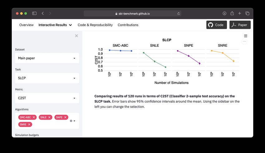
Benchmarking Simulation-Based Inference

led to independent development and co-existence of          simulation budgets, neural-network based approaches
closely-related algorithms in different disciplines.        outperform classical ABC algorithms, confirming re-
                                                            cent progress in the field; and 5) there is no algorithm
There are many exciting challenges and opportunities
                                                            to rule them all. The performance ranking of algo-
ahead, such as the scaling of these algorithms to high-
                                                            rithms is task-dependent, pointing to a need for better
dimensional data, active selection of simulations, and
                                                            guidance or automated procedures for choosing which
gray-box settings, as outlined in Cranmer et al. (2020).
                                                            algorithm to use when. We highlight examples of how
To tackle such challenges, researchers will need an ex-
                                                            the benchmark can be used to diagnose shortcomings of
tensible framework to compare existing algorithms and
                                                            algorithms and facilitate improvements. We end with
test novel ideas. Carefully curated, a benchmark frame-
                                                            a discussion of the limitations of the benchmark.
work will make it easier for researchers to enter SBI
research, and will fuel the development of new algo-
rithms through community involvement, exchange of           2     Benchmark
expertise and collaboration. Furthermore, benchmark-
ing results could help practitioners to decide which        The benchmark consists of a set of algorithms, per-
algorithm to use on a given problem of interest, and        formance metrics and tasks. Given a prior p(θ) over
thereby contribute to the dissemination of SBI.             parameters θ, a simulator to sample x ∼ p(x|θ) and
The catalyzing effect of benchmarks has been evident,       an observation xo , an algorithm returns an approxi-
e.g., in computer vision (Russakovsky et al., 2015),        mate posterior q(θ|xo ), or samples from it, θ ∼ q. The
speech recognition (Hirsch and Pearce, 2000; Wang           approximate solution is tested, according to a perfor-
et al., 2018), reinforcement learning (Bellemare et al.,    mance metric, against a reference posterior p(θ|xo ).
2013; Duan et al., 2016), Bayesian deep learning (Filos
et al., 2019; Wenzel et al., 2020), and many other fields   2.1   Algorithms
drawing on machine learning. Open benchmarks can
be an important component of transparent and repro-         Following the classification introduced in the review by
ducible computational research. Surprisingly, a bench-      Cranmer et al. (2020), we selected algorithms address-
mark framework for SBI has been lacking, possibly due       ing SBI in four distinct ways, as schematically depicted
to the challenging endeavor of designing benchmarking       in Fig. 1. An important difference between algorithms
tasks and defining suitable performance metrics.            is how new simulations are acquired: Sequential algo-
                                                            rithms adaptively choose informative simulations to
Here, we begin to address this challenge, and provide       increase sample efficiency. While crucial for expen-
a benchmark framework for SBI to allow rapid and            sive simulators, it can require non-trivial algorithmic
transparent comparisons of current and future SBI al-       steps and hyperparameter choices. To evaluate whether
gorithms: First, we selected a set of initial algorithms    the potential is realized empirically and justifies the
representing distinct approaches to SBI (Fig. 1; Cran-      algorithmic burden, we included sequential and non-
mer et al., 2020). Second, we analyzed multiple perfor-     sequential counterparts for algorithms of each category.
mance metrics which have been used in the SBI litera-
ture. Third, we implemented ten tasks including tasks       Keeping our initial selection focused allowed us to care-
popular in the field. The shortcomings of commonly          fully consider implementation details and hyperparam-
used metrics led us to focus on tasks for which a likeli-   eters: We extensively explored performance and sen-
hood can be evaluated, which allowed us to calculate        sitivity to different choices in more than 10k runs, all
reference (‘ground-truth’) posteriors. These reference      results and details of which can be found in Appendix H.
posteriors are made available to allow rapid evalua-        Our selection is briefly described below, full algorithm
tion of SBI algorithms. Code for the framework is           details are in Appendix A.
available at github.com/sbi-benchmark/sbibm and             REJ-ABC and SMC-ABC. Approximate Bayesian
we maintain an interactive version of all results at        Computation (ABC, Sisson et al., 2018) is centered
sbi-benchmark.github.io.                                    around the idea of Monte Carlo rejection sampling
The full potential of the benchmark will be real-           (Tavaré et al., 1997; Pritchard et al., 1999). Parameters
ized when it is populated with additional community-        θ are sampled from a proposal distribution, simulation
contributed algorithms and tasks. However, our initial      outcomes x are compared with observed data xo , and
version already provides useful insights: 1) the choice     are accepted or rejected depending on a (user-specified)
of performance metric is critical; 2) the performance of    distance function and rejection criterion. While rejec-
the algorithms on some tasks leaves substantial room        tion ABC (REJ-ABC) uses the prior as a proposal
for improvement; 3) sequential estimation generally         distribution, the efficiency can be improved by using
improves sample efficiency; 4) for small and moderate       sequentially refined proposal distributions (SMC-ABC,
                                                            Beaumont et al., 2002; Marjoram and Tavaré, 2006;
Jan-Matthis Lueckmann, Jan Boelts, David S. Greenberg, Pedro J. Gonçalves, Jakob H. Macke
Monte Carlo ABC Likelihood Estimation Posterior Estimation Ratio Estimation
prior prior proposal prior proposal prior proposal
sequential
proposal simulator simulator simulator
sequential
sequential
sequential
simulator likelihood est. posterior est. ratio est.
data compare infer data data evaluate infer data
posterior posterior posterior posterior
Figure 1: Overview of algorithms. We compare algorithms belonging to four distinct approaches to SBI:
Classical ABC approaches as well as model-based approaches approximating likelihoods, posteriors, or density
ratios. We contrast algorithms that use the prior distribution to propose parameters against ones that sequentially
adapt the proposal. Classification and schemes following Cranmer et al. (2020).
Sisson et al., 2007; Toni et al., 2009; Beaumont et al., NRE and SNRE. Ratio Estimation approaches to
2009). We implemented REJ-ABC with quantile-based SBI use classifiers to approximate density ratios (Izbicki
rejection and used the scheme of Beaumont et al. (2009) et al., 2014; Pham et al., 2014; Cranmer et al., 2015;
for SMC-ABC. We extensively varied hyperparameters Dutta et al., 2016; Durkan et al., 2020; Thomas et al.,
and compared the implementation of an ABC-toolbox 2020). Here, we used the recent approach proposed by
(Klinger et al., 2018) against our own (Appendix H). Hermans et al. (2020) as implemented in Durkan et al.
We investigated linear regression adjustment (Blum and (2020): A neural network-based classifier approximates
François, 2010) and the summary statistics approach probability ratios and MCMC is used to obtain samples
by Prangle et al. (2014) (Suppl. Fig. 1). from the posterior. SNRE denotes the sequential vari-
ant of neural ratio estimation (NRE). In Appendix H we
NLE and SNLE. Likelihood estimation (or ‘synthetic
compare different classifier architectures for (S)NRE.
likelihood’) algorithms learn an approximation to the
intractable likelihood, for an overview see Drovandi In addition, we benchmarked Random Forest ABC
et al. (2018). While early incarnations focused on (RF-ABC; Raynal et al., 2019), a recent ABC variant,
Gaussian approximations (SL; Wood, 2010), recent and Synthetic Likelihood (SL; Wood, 2010), mentioned
versions utilize deep neural networks (Papamakarios above. However, RF-ABC only targets individual pa-
et al., 2019b; Lueckmann et al., 2019) to approximate a rameters (i.e. assumes posteriors to factorize), and SL
density over x, followed by MCMC to obtain posterior requires new simulations for every MCMC step, thus
samples. Since we primarily focused on these latter requiring orders of magnitude more simulations than
versions, we refer to them as neural likelihood esti- other algorithms. Therefore, we report results for these
mation (NLE) algorithms, and denote the sequential algorithms separately, in Suppl. Fig. 2 and Suppl. Fig.
variant with proposals as SNLE. In particular, we used 3, respectively.
the scheme proposed by Papamakarios et al. (2019b)
Algorithms can be grouped with respect to how their
which uses masked autoregressive flows (MAFs, Pa-
output is represented: 1) some return samples from
pamakarios et al., 2017) for density estimation. We
the posterior, θ ∼ q(θ|xo ) (REJ-ABC, SMC-ABC); 2)
improved MCMC sampling for (S)NLE and compared
others return samples and allow evaluation of unnor-
MAFs against Neural Spline Flows (NSFs; Durkan
malized posteriors q̃(θ|xo ) ((S)NLE, (S)NRE); and 3)
et al., 2019), see Appendix H.
for some, the posterior density q(θ|xo ) can be evaluated
NPE and SNPE. Instead of approximating the like- and sampled directly, without MCMC ((S)NPE). As
lihood, these approaches directly target the posterior. discussed below, these properties constrain the metrics
Their origins date back to regression adjustment ap- that can be used for comparison.
proaches (Blum and François, 2010). Modern variants
(Papamakarios and Murray, 2016; Lueckmann et al.,
2.2 Performance metrics
2017; Greenberg et al., 2019) use neural networks for
density estimation (approximating a density over θ).
Choice of a suitable performance metric is central to
Here, we used the recent algorithmic approach proposed
any benchmark. As the goal of SBI algorithms is to
by Greenberg et al. (2019) for sequential acquisitions.
perform full inference, the ‘gold standard’ would be
We report performance using NSFs for density estima-
to quantify the similarity between the true posterior
tion, which outperformed MAFs (Appendix H).
and the inferred one with a suitable distance (or di-Benchmarking Simulation-Based Inference
vergence) measure on probability distributions. This choices, in particular on posteriors with multiple modes
would require both access to the ground-truth posterior, and length scales (see Results and Liu et al., 2020).
and a reliable means of estimating similarity between
Classifier 2-Sample Tests (C2ST). C2STs (Fried-
(potentially) richly structured distributions. Several
man, 2004; Lopez-Paz and Oquab, 2017) train a classi-
performance metrics have been used in past research,
fier to discriminate samples from the true and inferred
depending on the constraints imposed by knowledge
posteriors, which makes them simple to apply and easy
about ground-truth and the inference algorithm (see
to interpret. Therefore, we prefer to report and com-
Table 1). In real-world applications, typically only the
pare algorithms in terms of accuracy in classification-
observation xo is known. However, in a benchmarking
based tests. In the context of SBI, C2ST has e.g. been
setting, it is reasonable to assume that one has at least
used in Gutmann et al. (2018); Dalmasso et al. (2020).
access to the ground-truth parameters θ o . There are
two commonly used metrics which only require θ o and Other metrics that could be used include:
xo , but suffer severe drawbacks for our purposes:
Kernelized Stein Discrepancy (KSD). KSD (Liu
Probability θ o . The negative log probability et al., 2016; Chwialkowski et al., 2016) is a 1-sample test,
of true parameters averaged over different (θ o , xo ), which require access to ∇θ p̃(θ|xo ) rather than samples
−E[log q(θ o |xo )], has been used extensively in the liter- from p (p̃ is the unnormalized posterior). Like MMD,
ature (Papamakarios and Murray, 2016; Durkan et al., current estimators use translation-invariant kernels.
2018; Greenberg et al., 2019; Papamakarios et al., 2019b;
f -Divergences. Divergences such as Total Variation
Durkan et al., 2020; Hermans et al., 2020). Its appeal
(TV) divergence and KL divergences can only be com-
lies in the fact that one does not need access to the
puted when the densities of true and approximate pos-
ground-truth posterior. However, using it only for a
teriors can be evaluated (Table 1). Thus, we did not
small set of (θ o , xo ) is highly problematic: It is only a
use f -divergences for the benchmark.
valid performance measure if averaged over a large set of
observations sampled from the prior (Talts et al., 2018, Full discussion and details of metrics in Appendix M.
detailed discussion including connection to simulation-
based calibration in Appendix M). For reliable results, 2.3 Tasks
one would require inference for hundreds of xo which
is only feasible if inference is rapid (amortized) and The preceding considerations guided our selection of
the density q can be evaluated directly (among the inference tasks: We focused on tasks for which reference
algorithms used here this applies only to NPE). posterior samples θ ∼ p can be obtained, to allow
calculation of 2-sample tests. We focused on eight
Posterior-Predictive Checks (PPCs). As the purely statistical problems and two problems relevant
name implies, PPCs should be considered a mere check in applied domains, with diverse dimensionalities of
rather than a metric, although the median distance be- parameters and data (details in Appendix T):
tween predictive samples and xo has been reported in
the SBI literature (Papamakarios et al., 2019b; Green- Gaussian Linear/Gaussian Linear Uniform. We
berg et al., 2019; Durkan et al., 2020). A failure mode included two versions of simple, linear, 10-d Gaussian
of such a metric is that an algorithm obtaining a good models, in which the parameter θ is the mean, and the
MAP point estimate, could perfectly pass this check covariance is fixed. The first version has a Gaussian
even if the estimated posterior is poor. Empirically, we (conjugate) prior, the second one a uniform prior. These
found median-distances (MEDDIST) to be in disagree- tasks allow us to test how algorithms deal with trivial
ment with other metrics (see Results). scaling of dimensionality, as well as truncated support.
The shortcomings of these commonly-used metrics led SLCP/SLCP Distractors. A challenging inference
us to focus on tasks for which it is possible to get sam- task designed to have a simple likelihood and a complex
ples from ground-truth posterior θ ∼ p, thus allowing posterior (Papamakarios et al., 2019b; Greenberg et al.,
us to use metrics based on two-sample tests: 2019): The prior is uniform over five parameters θ
and the data are a set of four two-dimensional points
Maximum Mean Discrepancy (MMD). MMD sampled from a Gaussian likelihood whose mean and
(Gretton et al., 2012; Sutherland et al., 2017) is a variance are nonlinear functions of θ. This induces a
kernel-based 2-sample test. Recent papers (Papamakar- complex posterior with four symmetrical modes and
ios et al., 2019b; Greenberg et al., 2019; Hermans et al., vertical cut-offs. We included a second version with
2020) reported MMD using translation-invariant Gaus- 92 additional, non-informative outputs (distractors) to
sian kernels with length scales determined by the me- test the ability to detect informative features.
dian heuristic (Ramdas et al., 2015). We empirically
found that MMD can be sensitive to hyperparameter Bernoulli GLM/Bernoulli GLM Raw. 10-
parameter Generalized Linear Model (GLM) withJan-Matthis Lueckmann, Jan Boelts, David S. Greenberg, Pedro J. Gonçalves, Jakob H. Macke
Table 1: Applicability of metrics given knowledge about ground truth and algorithm. Whether a
metric can be used depends on both what is known about the ground-truth of an inference task and what an
algorithm returns: Information about ground truth can vary between just having observed data xo (typical setting
in practice), knowing the generating parameter θ o , having posterior samples, gradients, or being able to evaluate
the true posterior p. Tilde denotes unnormalized distributions. Access to information is cumulative.
Ground truth →
↓ Algorithm xo θo θ∼p ∇p̃(θ|xo ) p(θ|xo )
θ∼q 1 1 1, 3 1, 3, 4 1, 3, 4
q̃(θ|xo ) 1 1 1, 3 1, 3, 4 1, 3, 4
q(θ|xo ) 1 1, 2 1, 2, 3 1, 2, 3, 4 1, 2, 3, 4, 5
1 = PPCs, 2 = Probability θ 0 , 3 = 2-sample tests, 4 = 1-sample tests, 5 = f -divergences.
Bernoulli observations. Inference was either performed For each observation, each algorithm was run with a
on sufficient statistics (10-d) or raw data (100-d). simulation budget ranging from 1k to 100k simulations.
Gaussian Mixture. This inference task, introduced For each run, we calculated metrics described above.
by Sisson et al. (2007), has become common in the To estimate C2ST accuracy, we trained a multilayer
ABC literature (Beaumont et al., 2009; Toni et al., perceptron to tell apart approximate and reference pos-
2009; Simola et al., 2020). It consists of a mixture of terior samples and performed five-fold cross-validation.
two two-dimensional Gaussian distributions, one with We used two hidden layers, each with 10 times as many
much broader covariance than the other. ReLu units as the dimensionality of the data. We also
measured and report runtimes (Appendix R).
Two Moons. A two-dimensional task with a poste-
rior that exhibits both global (bimodality) and local
(crescent shape) structure (Greenberg et al., 2019) to 2.5 Software
illustrate how algorithms deal with multimodality.
SIR. Dynamical systems represent paradigmatic use Code. All code is released publicly at
cases for SBI. SIR is an influential epidemiological github.com/sbi-benchmark/sbibm. Our frame-
model describing the dynamics of the number of indi- work includes tasks, reference posteriors, metrics,
viduals in three possible states: susceptible S, infectious plotting, and infrastructure tooling and is designed to
I, and recovered or deceased, R. We infer the contact be 1) easily extensible, 2) used with external toolboxes
rate β and the mean recovery rate γ, given observed implementing algorithms. All tasks are implemented
infection counts I at 10 evenly-spaced time points. as probabilistic programs in Pyro (Bingham et al.,
2019), so that likelihoods and gradients for reference
Lotka-Volterra. An influential model in ecology de- posteriors can be extracted automatically. To make
scribing the dynamics of two interacting species, widely this possible for tasks that use ODEs, we developed
used in SBI studies. We infer four parameters θ related a new interface between DifferentialEquations.jl
to species interaction, given the number of individuals (Rackauckas and Nie, 2017; Bezanson et al., 2017) and
in both populations at 10 evenly-spaced points in time. PyTorch (Paszke et al., 2019). In addition, specifying
simulators in a probabilistic programming language
has the advantage that ‘gray-box’ algorithms (Brehmer
2.4 Experimental Setup
et al., 2020; Cranmer et al., 2020) can be added in the
future. We here evaluated algorithms implemented
For each task, we sampled 10 sets of true parameters
in pyABC (Klinger et al., 2018), pyabcranger (Collin
from the prior and generated corresponding observa-
et al., 2020), and sbi (Tejero-Cantero et al., 2020).
tions (θ o , xo )1:10 . For each observation, we generated
See Appendix B for details and existing SBI toolboxes.
10k samples from the reference posterior. Some refer-
ence posteriors required a customised (likelihood-based) Reproducibility. Instructions to reproduce experi-
approach (Appendix B). ments on cloud-based infrastructure are in Appendix B.
In SBI, it is typically assumed that total computation Website. Along with the code, we provide a web
cost is dominated by simulation time. We therefore interface which allows interactive exploration of all the
report performance at different simulation budgets. results (sbi-benchmark.github.io; Appendix W).Benchmarking Simulation-Based Inference
Two Moons
REJ�ABC NLE NPE NRE SMC�ABC SNLE SNPE SNRE
1.0
0.9
C2ST
0.8
0.7
0.6
0.5 Two Moons
10³
10⁴
10⁵
10³
10⁴
10⁵
10³
10⁴
10⁵
10³
10⁴
10⁵
10³
10⁴
10⁵
10³
10⁴
10⁵
10³
10⁴
10⁵
10³
10⁴
10⁵
0.08
MMD²
Number of Simulations
0.04
0.00 Two Moons
10³
10⁴
10⁵
10³
10⁴
10⁵
10³
10⁴
10⁵
10³
10⁴
10⁵
10³
10⁴
10⁵
10³
10⁴
10⁵
10³
10⁴
10⁵
10³
10⁴
10⁵
0.24
MEDDIST
0.20
Number of Simulations
0.16
0.12
0.08
10³
10⁴
10⁵
10³
10⁴
10⁵
10³
10⁴
10⁵
10³
10⁴
10⁵
10³
10⁴
10⁵
10³
10⁴
10⁵
10³
10⁴
10⁵
10³
10⁴
10⁵
Number of Simulations
Figure 2: Performance on Two Moons according to various metrics. Best possible performance would be
0.5 for C2ST, 0 for MMD2 and MEDDIST. Results for 10 observations each, means and 95% confidence intervals.
3 Results Based on the comparison of the performance across all
tasks, we highlight the following main points:
We first consider empirical results on a single task, Two #2: These are not solved problems. C2ST uses
Moons, according to different metrics, which illustrate an interpretable scale (1 to 0.5), which makes it possible
the following important insight: to conclude that, for several tasks, no algorithm could
#1: Choice of performance metric is key. While solve them with the specified budget (e.g., SLCP, Lotka-
C2ST results on Two Moons show that performance Volterra). This highlights that our problems—though
increases with higher simulation budgets and that se- conceptually simple—are challenging, and there is room
quential algorithms outperform non-sequential ones for for development of more powerful algorithms.
low to medium budgets, these results were not reflected #3: Sequential estimation improves sample ef-
in MMD and MEDDIST (Fig. 2): In our analyses, we ficiency. Our results show that sequential algorithms
found MMD to be sensitive to hyperparameter choices, outperform non-sequential ones (Fig. 3). The differ-
in particular on tasks with complex posterior struc- ence was small on simple tasks (i.e. linear Gaussian
ture. When using the commonly employed median cases), yet pronounced on most others. However, we
heuristic to set the kernel length scale on a task with also found these methods to exhibit diminishing re-
multi-modal posteriors (like Two Moons), MMD had turns as the simulation budget grows, which points to
difficulty discerning markedly different posteriors. This an opportunity for future improvements.
can be ‘fixed’ by using hyperparameters adapted to the
task (Suppl. Fig. 4). As discussed above, the median #4: Density or ratio estimation-based al-
distance (though commonly used) can be ‘gamed’ by gorithms generally outperform classical tech-
a good point estimate even if the estimated posterior niques. REJ-ABC and SMC-ABC were generally
is poor and is thus not a suitable performance metric. outperformed by more recent techniques which use
Computation of KSD showed numerical problems on neural networks for density- or ratio-estimation, and
Two Moons, due to the gradient calculation. which can therefore efficiently interpolate between dif-
ferent simulations (Fig. 3). Without such model-based
We assessed relationships between metrics empirically interpolation, even a simple 10-d Gaussian task can be
via the correlations across tasks (Suppl. Fig. 5). As challenging. However, classical rejection-based meth-
discussed above, the log-probability of ground-truth ods have a computational footprint that is orders of
parameters can be problematic when averaged over magnitudes smaller, as no network training is involved
too few observations (e.g., 10, as is common in the (Appendix R). Thus, on low-dimensional problems and
literature): indeed, this metric had a correlation of for cheap simulators, these methods can still be com-
only 0.3 with C2ST on Two Moons and 0.6 on the petitive. See Suppl. Fig. 1 for results with additional
SLCP task. Based on these considerations, we used ABC variants (Blum and François, 2010; Prangle et al.,
C2ST for reporting performance (Fig. 3; results for 2014) and Suppl. Fig. 2 for results on RF-ABC.
MMD, KSD and median distance on the website).Jan-Matthis Lueckmann, Jan Boelts, David S. Greenberg, Pedro J. Gonçalves, Jakob H. Macke
● Gaussian Linear / ■ Gaussian Linear Uniform
REJ�ABC NLE NPE NRE SMC�ABC SNLE SNPE SNRE
1.0
0.9
C2ST
0.8
0.7
0.6
0.5
10³
10⁴
10⁵
10³
10⁴
10⁵
10³
10⁴
10⁵
10³
10⁴
10⁵
10³
10⁴
10⁵
10³
10⁴
10⁵
10³
10⁴
10⁵
10³
10⁴
10⁵
● SLCP / ■ SLCP Distractors
1.0 Number of Simulations
0.9
C2ST
0.8
0.7
0.6
0.5
10³
10⁴
10⁵
10³
10⁴
10⁵
10³
10⁴
10⁵
10³
10⁴
10⁵
10³
10⁴
10⁵
10³
10⁴
10⁵
10³
10⁴
10⁵
10³
10⁴
10⁵
● Bernoulli GLM / ■ Bernoulli GLM Raw
1.0 Number of Simulations
0.9
C2ST
0.8
0.7
0.6
0.5
10³
10⁴
10⁵
10³
10⁴
10⁵
10³
10⁴
10⁵
10³
10⁴
10⁵
10³
10⁴
10⁵
10³
10⁴
10⁵
10³
10⁴
10⁵
10³
10⁴
10⁵
Gaussian Mixture
1.0 Number of Simulations
0.9
C2ST
0.8
0.7
0.6
0.5
10³
10⁴
10⁵
10³
10⁴
10⁵
10³
10⁴
10⁵
10³
10⁴
10⁵
10³
10⁴
10⁵
10³
10⁴
10⁵
10³
10⁴
10⁵
10³
10⁴
10⁵
SIR
1.0 Number of Simulations
0.9
C2ST
0.8
0.7
0.6
0.5
10³
10⁴
10⁵
10³
10⁴
10⁵
10³
10⁴
10⁵
10³
10⁴
10⁵
10³
10⁴
10⁵
10³
10⁴
10⁵
10³
10⁴
10⁵
10³
10⁴
10⁵
Lotka-Volterra
1.0 Number of Simulations
0.9
C2ST
0.8
0.7
0.6
0.5
10³
10⁴
10⁵
10³
10⁴
10⁵
10³
10⁴
10⁵
10³
10⁴
10⁵
10³
10⁴
10⁵
10³
10⁴
10⁵
10³
10⁴
10⁵
10³
10⁴
10⁵
Number of Simulations
Figure 3: Performance on other benchmark tasks. Classification accuracy (C2ST) of REJ-ABC, SMC-ABC,
NLE, SNLE, NPE, SNPE, NRE, SNRE for 10 observations each, means and 95% confidence intervals.
#5: No one algorithm to rule them all. Al- terior can help identify and improve such issues: We
though sequential density or ratio estimation-based found that single chains initialized by sampling from
algorithms performed better than their non-sequential the prior with axis-aligned slice sampling (as intro-
counterparts, there was no clear-cut answer as to which duced in Papamakarios et al., 2019b) frequently got
sequential method (SNLE, SNRE, and SNPE) should stuck in single modes. Based on this observation, we
be preferred. To some degree, this is to be expected: changed the MCMC strategy (details in Appendix A),
these algorithms have distinct strengths that can play which, though simple, yielded significant performance
out differently depending on the problem structure (see and speed improvements on the benchmark tasks. Sim-
discussions e.g., in Greenberg et al., 2019; Durkan et al., ilarly, (S)NLE and (S)NRE improved by transforming
2018, 2020). However, this has not been shown system- parameters to be unbounded: Without transforma-
atically before. We formulate some practical guidelines tions, runs on some tasks can get stuck during MCMC
for choosing appropriate algorithms in Box 1. sampling (e.g., Lotka-Volterra). While this is com-
mon advice for MCMC (Hogg and Foreman-Mackey,
#6: The benchmark can be used to diagnose
2018), it has been lacking in code and papers of SBI
implementation issues and improve algorithms.
approaches.
For example, (S)NLE and (S)NRE rely on MCMC sam-
pling to compute posteriors, and this sampling step We used the benchmark to systematically compare
can limit the performance. Access to a reference pos- hyperparameters: For example, as density estimatorsBenchmarking Simulation-Based Inference
Do we need the Bayesian posterior, or is a point estimate sufficient?
Our focus was on SBI algorithms that target the Bayesian posterior. If one only aims for a single estimate,
optimization methods (e.g. Rios and Sahinidis, 2013; Shahriari et al., 2015) might be more efficient.
Is the simulator really ‘black-box’ ?
The SBI algorithms presented in the benchmark can be applied to any ‘black-box’ simulator. However,
if the likelihood is available, methods exploiting it (e.g. MCMC, variational inference) will generally be
more efficient. Similarly, if one has access to the internal random numbers, probabilistic programming
approaches (Le et al., 2017; Baydin et al., 2019; Wood et al., 2020) might be preferable. If additional
quantities that characterize the latent process are available, i.e., the simulator is ‘gray-box’, they can be
used to augment training data and improve inference (Brehmer et al., 2020; Cranmer et al., 2020).
What domain knowledge do we have about the problem?
For any practical application of SBI, it is worth thinking carefully about domain knowledge. First,
knowledge about plausible parameters should inform the choice of the prior. Second, domain knowledge
can help design appropriate distance functions or summary statistics required for classical ABC algorithms.
When using model-based approaches, domain knowledge can potentially be built into the SBI algorithm
itself, for example, by incorporating neural network layers with appropriate inductive biases or invariances.
Do we have, or can we learn summary statistics?
Summary statistics are especially important when facing problems with high-dimensional data: It is
important to point out that the posterior given summary statistics p(θ|s(xo )) is only equivalent to p(θ|xo )
if the summary statistics are sufficient. The problem at hand can guide the manual design of summary
statistics that are regarded particularly important or informative. Alternatively, many automatic approaches
exist (e.g., Prangle et al., 2014; Charnock et al., 2018; Dinev and Gutmann, 2018) and this is an active
area of research (e.g., Chen et al. 2021 recently proposed an approach to learn approximately sufficient
statistics for SMC-ABC and (S)NLE). (S)NPE and (S)NRE can directly reduce high-dimensional data as
part of their network architectures.
Do we have low-dimensional data and parameters, and a cheap simulator?
If both the parameters and the data (or suitable summary-statistics thereof) are low-dimensional, and
a very large number of simulations can be generated, model-free algorithms such as classical ABC can
be competitive. These have the benefit of adding little computational overhead. Conversely, for limited
simulation budgets and/or higher dimensionalities, approaches that train a model of the likelihood, posterior,
or likelihood ratio will generally be preferable.
Are simulations expensive? Can we simulate online?
For time-intensive and complex simulators, it can be beneficial to use sequential methods to increase sample
efficiency: We found that sequential schemes generally outperformed non-sequential ones. While we focused
on simple strategies which use the previous estimate of the posterior to propose new parameters, more
sophisticated schemes (e.g., Gutmann and Corander, 2016; Lueckmann et al., 2019; Järvenpää et al., 2019)
may increase sample efficiency if only few simulations can be obtained. For some applications, inference is
performed on a fixed dataset, and one cannot resort to sequential algorithms.
Do we want to carry out inference once, or repeatedly?
To perform SBI separately for different data points (i.e. compute p(θ|x1 ), p(θ|x2 ), . . .), methods that allow
‘amortization’ (NPE) are likely preferable. While NLE and NRE allow amortisation of the neural network,
MCMC sampling is required, which takes additional time. Conversely, if we want to run SBI conditioned
on many i.i.d. data (e.g. p(θ|x1 , x2 , . . .)) methods based on likelihood or ratio estimation (NLE, NRE), or
NPE with exchangeable neural networks (Chan et al., 2018) would be appropriate.
Box 1: Practitioners’ advice for applying SBI algorithms. Based on our current results and understanding,
we provide advice to practitioners seeking to apply SBI. There is no one-fits-all solution—which algorithm to use
in practice will depend on the problem at hand. For additional advice, see Cranmer et al. (2020).Jan-Matthis Lueckmann, Jan Boelts, David S. Greenberg, Pedro J. Gonçalves, Jakob H. Macke
for (S)NLE and (S)NPE, we used NSFs (Durkan et al., lems for which reference posteriors can be computed.
2020) which were developed after these algorithms were This raises the question of how insights on these prob-
published. This revealed that higher capacity density lems will generalize to ‘real-world’ simulators. Notably,
estimators were beneficial for posterior but not likeli- even these simple problems already identify clear dif-
hood estimation (detailed analysis in Appendix H). ferences between, and limitations of, different SBI ap-
proaches. Since it is not possible to rigorously compare
These examples show how the benchmark makes it
the performance of different algorithms directly on ‘real-
possible to diagnose problems and improve algorithms.
world’ simulators due to the lack of appropriate metrics,
we see the benchmark as a necessary stepping stone
4 Limitations towards the development of (potentially automated)
selection strategies for practical problems.
Our benchmark, in its current form, has several limi-
tations. First, the algorithms considered here do not Sixth, in practice, the choice of algorithm can depend
cover the entire spectrum of SBI algorithms: We did on aspects that are difficult to quantify: It will depend
not include sequential algorithms using active learning on the available information about a problem, the in-
or Bayesian Optimization (Gutmann and Corander, ference goal, and the speed of the simulator, among
2016; Järvenpää et al., 2019; Lueckmann et al., 2019; other considerations. We included some practical con-
Aushev et al., 2020), or ‘gray-box’ algorithms, which siderations and recommendations in Box 1.
use additional information about or from the simula- Finally, benchmarking is an important tool, but not
tor (e.g., Baydin et al., 2019; Brehmer et al., 2020). an end in itself—for example, conceptually new ideas
We focused on approaches using neural networks for might initially not yield competitive results but only
density estimation and did not compare to alternatives reveal their true value later. Conversely, ‘overfitting’
using Gaussian Processes (e.g., Meeds and Welling, on benchmarks can lead to the illusion of progress,
2014; Wilkinson, 2014). There are many other algo- and result in an undue focus on small implementation
rithms which the benchmark is currently lacking (e.g., details which might not generalize beyond it. It would
Nott et al., 2014; Ong et al., 2018; Clarté et al., 2020; certainly be possible to cheat on this benchmark: In
Prangle, 2019; Priddle et al., 2019; Picchini et al., 2020; particular, as the simulators are available, one could use
Radev et al., 2020; Rodrigues et al., 2020). Keeping samples (or even likelihoods) to excessively tune hyper-
our initial selection small allowed us to carefully investi- parameters for each task. This would hardly transfer to
gate hyperparameter choices. We focused on sequential practice where such tuning is usually impossible (lack of
algorithms with less sophisticated acquisition schemes metrics and expensive simulators). Therefore, we care-
and the black-box scenario, since we think these are fully compared choices and selected hyperparameters
important baselines for future comparisons. performing best across tasks (Appendix H).
Second, the tasks we considered do not cover the vari-
ety of possible challenges. Notably, while we have tasks 5 Discussion
with high dimensional data with and without structure,
we have not included tasks with high-dimensional spa- Quantitatively evaluating, comparing and improving
tial structure, e.g., images. Such tasks would require algorithms through benchmarking is at the core of
algorithms that automatically learn summary statistics progress in machine learning. We here provided an
while exploring the structure of the data (e.g., Dinev initial benchmark for simulation-based inference. If
and Gutmann, 2018; Greenberg et al., 2019; Hermans used sensibly, it will be an important tool for clari-
et al., 2020; Chen et al., 2021), an active research area. fying and expediting progress in SBI. We hope that
the current results on multiple widely-used algorithms
Third, while we extensively investigated tuning choices
already provide insights into the state of the field, assist
and compared implementations, the results might nev-
researchers with algorithm development, and that our
ertheless reflect our own areas of expertise.
recommendations for practitioners will help them in
Fourth, in line with common practice in SBI, results selecting appropriate algorithms.
presented in the paper focused on performance as a
We believe that the full potential of the benchmark
function of the number of simulation calls. It is impor-
will be revealed as more researchers participate and
tant to remember that differences in computation time
contribute. To facilitate this process, and allow users
can be substantial (see Appendix R): For example,
to quickly explore and compare algorithms, we are
(S)ABC was much faster than approaches requiring
providing precomputed reference posteriors, a website
network training. Overall, sequential neural algorithms
(sbi-benchmark.github.io), and open-source code
exhibited longest runtimes.
(github.com/sbi-benchmark/sbibm).
Fifth, for reasons described above, we focused on prob-Benchmarking Simulation-Based Inference
Acknowledgements C. P. Robert
2009. Adaptive approximate bayesian computation.
We thank Álvaro Tejero-Cantero, Auguste Schulz, Biometrika, 96(4):983–990.
Conor Durkan, François Lanusse, Leandra White, Mar- Beaumont, M. A., W. Zhang, and D. J. Balding
cel Nonnenmacher, Michael Deistler, Pedro Rodrigues, 2002. Approximate bayesian computation in popula-
Poornima Ramesh, Sören Becker and Theofanis Kar- tion genetics. Genetics, 162(4):2025–2035.
aletsos for discussions and comments on the manuscript.
Bellemare, M. G., Y. Naddaf, J. Veness, and M. Bowl-
In addition, J.-M.L. would like to thank the organisers
ing
and participants of the Likelihood-Free Inference Work-
2013. The arcade learning environment: An evalua-
shop hosted by the Simons Foundation for discussions,
tion platform for general agents. Journal of Artificial
in particular, Danley Hsu, François Lanusse, George
Intelligence Research, 47:253–279.
Papamakarios, Henri Pesonen, Joeri Hermans, Johann
Brehmer, Kyle Cranmer, Owen Thomas and Umberto Bezanson, J., A. Edelman, S. Karpinski, and V. B.
Simola. We also acknowledge and thank the Python Shah
(Van Rossum and Drake Jr, 1995) and Julia (Bezanson 2017. Julia: A fresh approach to numerical comput-
et al., 2017) communities for developing the tools en- ing. SIAM review, 59(1):65–98.
abling this work, including Altair (VanderPlas et al., Bingham, E., J. P. Chen, M. Jankowiak, F. Obermeyer,
2018), DifferentialEquations.jl (Rackauckas and N. Pradhan, T. Karaletsos, R. Singh, P. Szerlip,
Nie, 2017), Hydra (Yadan, 2019), kernel-gof (Jitkrit- P. Horsfall, and N. D. Goodman
tum et al., 2017), igms (Sutherland, 2017), NumPy 2019. Pyro: Deep universal probabilistic pro-
(Harris et al., 2020), pandas (pandas development gramming. Journal of Machine Learning Research,
team, 2020), pyABC (Klinger et al., 2018), pyabcranger 20(1):973–978.
(Collin et al., 2020), Pyro (Bingham et al., 2019), Blum, M. G. and O. François
PyTorch (Paszke et al., 2019), sbi (Tejero-Cantero 2010. Non-linear regression models for approximate
et al., 2020), Scikit-learn (Pedregosa et al., 2011), bayesian computation. Statistics and Computing,
torch-two-sample (Djolonga, 2017), and vega-lite 20(1):63–73.
(Satyanarayan et al., 2017).
Brehmer, J., K. Cranmer, G. Louppe, and J. Pavez
This work was supported by the German Research 2018. Constraining effective field theories with
Foundation (DFG; SFB 1233 PN 276693517, SFB 1089, machine learning. Physical Review Letters,
SPP 2041, Germany’s Excellence Strategy – EXC num- 121(11):111801.
ber 2064/1 PN 390727645) and the German Federal Brehmer, J., G. Louppe, J. Pavez, and K. Cranmer
Ministry of Education and Research (BMBF; project 2020. Mining gold from implicit models to improve
’ADIMEM’, FKZ 01IS18052 A-D). likelihood-free inference. Proceedings of the National
Academy of Sciences, 117(10):5242–5249.
References
Chan, J., V. Perrone, J. Spence, P. Jenkins, S. Math-
Alsing, J., B. Wandelt, and S. Feeney ieson, and Y. Song
2018. Massive optimal data compression and density 2018. A likelihood-free inference framework for pop-
estimation for scalable, likelihood-free inference in ulation genetic data using exchangeable neural net-
cosmology. Monthly Notices of the Royal Astronomi- works. In Advances in Neural Information Processing
cal Society, 477(3):2874–2885. Systems 31, Pp. 8594–8605. Curran Associates, Inc.
Aushev, A., H. Pesonen, M. Heinonen, J. Corander, Charnock, T., G. Lavaux, and B. D. Wandelt
and S. Kaski 2018. Automatic physical inference with information
2020. Likelihood-free inference with deep gaussian maximizing neural networks. Physical Review D,
processes. Deep Learning and Inverse Problems 97(8):083004.
Workshop at Neural Information Processing Systems. Chen, Y., D. Zhang, M. Gutmann, A. Courville, and
Baydin, A. G., L. Shao, W. Bhimji, L. Heinrich, Z. Zhu
L. Meadows, J. Liu, A. Munk, S. Naderiparizi, 2021. Neural approximate sufficient statistics for im-
B. Gram-Hansen, G. Louppe, et al. plicit models. In Proceedings of the 9th International
2019. Etalumis: bringing probabilistic programming Conference on Learning Representations, ICLR.
to scientific simulators at scale. In Proceedings of Chwialkowski, K., H. Strathmann, and A. Gretton
the International Conference for High Performance 2016. A kernel test of goodness of fit. In Proceed-
Computing, Networking, Storage and Analysis, Pp. 1– ings of The 33rd International Conference on Ma-
24. chine Learning, volume 48 of Proceedings of Machine
Beaumont, M. A., J.-M. Cornuet, J.-M. Marin, and Learning Research, Pp. 2606–2615. PMLR.Jan-Matthis Lueckmann, Jan Boelts, David S. Greenberg, Pedro J. Gonçalves, Jakob H. Macke
Clarté, G., C. P. Robert, R. J. Ryder, and J. Stoehr Durkan, C., G. Papamakarios, and I. Murray
2020. Component-wise approximate bayesian com- 2018. Sequential neural methods for likelihood-free
putation via gibbs-like steps. Biometrika. inference. Bayesian Deep Learning Workshop at
Neural Information Processing Systems.
Collin, F.-D., A. Estoup, J.-M. Marin, and L. Raynal
2020. Bringing abc inference to the machine learn- Dutta, R., J. Corander, S. Kaski, and M. U. Gutmann
ing realm: Abcranger, an optimized random forests 2016. Likelihood-free inference by ratio estimation.
library for abc. In JOBIM 2020, volume 2020. arXiv preprint arXiv:1611.10242.
Filos, A., S. Farquhar, A. N. Gomez, T. G. Rudner,
Cranmer, K., J. Brehmer, and G. Louppe
Z. Kenton, L. Smith, M. Alizadeh, A. de Kroon, and
2020. The frontier of simulation-based inference.
Y. Gal
Proceedings of the National Academy of Sciences.
2019. A systematic comparison of bayesian deep
Cranmer, K., J. Pavez, and G. Louppe learning robustness in diabetic retinopathy tasks.
2015. Approximating likelihood ratios with cal- Bayesian Deep Learning Workshop at Neural Infor-
ibrated discriminative classifiers. arXiv preprint mation Processing Systems.
arXiv:1506.02169. Friedman, J.
Dalmasso, N., A. B. Lee, R. Izbicki, T. Pospisil, and 2004. On multivariate goodness-of-fit and two-sample
C.-A. Lin testing. In Conference on Statistical Problems in
2020. Validation of approximate likelihood and em- Particle Physics, Astrophysics and Cosmology.
ulator models for computationally intensive simu- Gonçalves, P. J., J.-M. Lueckmann, M. Deistler,
lations. In Proceedings of The 23rd International M. Nonnenmacher, K. Öcal, G. Bassetto, C. Chin-
Conference on Artificial Intelligence and Statistics taluri, W. F. Podlaski, S. A. Haddad, T. P. Vogels,
(AISTATS). D. S. Greenberg, and J. H. Macke
Dinev, T. and M. U. Gutmann 2020. Training deep neural density estimators to iden-
2018. Dynamic likelihood-free inference via ratio tify mechanistic models of neural dynamics. eLife.
estimation (dire). arXiv preprint arXiv:1810.09899. Gourieroux, C., A. Monfort, and E. Renault
1993. Indirect inference. Journal of Applied Econo-
Djolonga, J. metrics, 8(S1):S85–S118.
2017. torch-two-sample: A pytorch library for differ-
entiable two-sample tests. Github. Greenberg, D., M. Nonnenmacher, and J. Macke
2019. Automatic posterior transformation for
Drovandi, C. C., C. Grazian, K. Mengersen, and likelihood-free inference. In Proceedings of the 36th
C. Robert International Conference on Machine Learning, vol-
2018. Approximating the likelihood in approximate ume 97 of Proceedings of Machine Learning Research,
bayesian computation. In Handbook of Approxi- Pp. 2404–2414. PMLR.
mate Bayesian Computation, S. Sisson, Y. Fan, and
Gretton, A., K. M. Borgwardt, M. J. Rasch,
M. Beaumont, eds., chapter 12. CRC Press, Taylor
B. Schölkopf, and A. Smola
& Francis Group.
2012. A kernel two-sample test. The Journal of
Duan, Y., X. Chen, R. Houthooft, J. Schulman, and Machine Learning Research, 13(Mar):723–773.
P. Abbeel Gutmann, M. U. and J. Corander
2016. Benchmarking deep reinforcement learning 2016. Bayesian optimization for likelihood-free in-
for continuous control. In Proceedings of the 33th ference of simulator-based statistical models. The
International Conference on Machine Learning, vol- Journal of Machine Learning Research, 17(1):4256–
ume 48 of Proceedings of Machine Learning Research, 4302.
Pp. 1329–1338. PMLR.
Gutmann, M. U., R. Dutta, S. Kaski, and J. Corander
Durkan, C., A. Bekasov, I. Murray, and G. Papamakar- 2018. Likelihood-free inference via classification.
ios Statistics and Computing, 28(2):411–425.
2019. Neural spline flows. In Advances in Neu- Harris, C. R., K. J. Millman, S. J. van der Walt,
ral Information Processing Systems, Pp. 7509–7520. R. Gommers, P. Virtanen, D. Cournapeau, E. Wieser,
Curran Associates, Inc. J. Taylor, S. Berg, N. J. Smith, et al.
Durkan, C., I. Murray, and G. Papamakarios 2020. Array programming with numpy. Nature,
2020. On contrastive learning for likelihood-free in- 585(7825):357–362.
ference. In Proceedings of the 36th International Hermans, J., V. Begy, and G. Louppe
Conference on Machine Learning, volume 98 of Pro- 2020. Likelihood-free mcmc with approximate likeli-
ceedings of Machine Learning Research. PMLR. hood ratios. In Proceedings of the 37th InternationalBenchmarking Simulation-Based Inference
Conference on Machine Learning, volume 98 of Pro- Conference on Machine Learning, volume 48 of Pro-
ceedings of Machine Learning Research. PMLR. ceedings of Machine Learning Research, Pp. 276–284.
PMLR.
Hirsch, H.-G. and D. Pearce
2000. The aurora experimental framework for the per- Lopez-Paz, D. and M. Oquab
formance evaluation of speech recognition systems un- 2017. Revisiting classifier two-sample tests. In 5th In-
der noisy conditions. In ASR2000-Automatic Speech ternational Conference on Learning Representations,
Recognition: Challenges for the new Millenium ISCA ICLR.
Tutorial and Research Workshop (ITRW).
Lueckmann, J.-M., G. Bassetto, T. Karaletsos, and
Hogg, D. W. and D. Foreman-Mackey J. H. Macke
2018. Data analysis recipes: Using markov chain 2019. Likelihood-free inference with emulator net-
monte carlo. The Astrophysical Journal Supplement works. In Proceedings of The 1st Symposium on
Series, 236(1):11. Advances in Approximate Bayesian Inference, vol-
Izbicki, R., A. Lee, and C. Schafer ume 96 of Proceedings of Machine Learning Research,
2014. High-dimensional density ratio estimation with Pp. 32–53. PMLR.
extensions to approximate likelihood computation. Lueckmann, J.-M., P. J. Goncalves, G. Bassetto,
In Artificial Intelligence and Statistics, Pp. 420–429. K. Öcal, M. Nonnenmacher, and J. H. Macke
Järvenpää, M., M. U. Gutmann, A. Pleska, A. Vehtari, 2017. Flexible statistical inference for mechanistic
P. Marttinen, et al. models of neural dynamics. In Advances in Neural
2019. Efficient acquisition rules for model-based ap- Information Processing Systems 30, Pp. 1289–1299.
proximate bayesian computation. Bayesian Analysis, Curran Associates, Inc.
14(2):595–622. Marjoram, P. and S. Tavaré
Järvenpää, M., M. U. Gutmann, A. Vehtari, P. Martti- 2006. Modern computational approaches for
nen, et al. analysing molecular genetic variation data. Nature
2020. Parallel gaussian process surrogate bayesian Reviews Genetics, 7(10):759–770.
inference with noisy likelihood evaluations. Bayesian Meeds, E. and M. Welling
Analysis. 2014. Gps-abc: Gaussian process surrogate approx-
Jitkrittum, W., W. Xu, Z. Szabó, K. Fukumizu, and imate bayesian computation. In Proceedings of the
A. Gretton Thirtieth Conference on Uncertainty in Artificial In-
2017. A linear-time kernel goodness-of-fit test. In telligence, UAI’14, P. 593–602, Arlington, Virginia,
Advances in Neural Information Processing Systems, USA. AUAI Press.
Pp. 262–271. Nott, D. J., Y. Fan, L. Marshall, and S. Sisson
Karabatsos, G. and F. Leisen 2014. Approximate bayesian computation and
2018. An approximate likelihood perspective on abc bayes’ linear analysis: toward high-dimensional abc.
methods. Statistics Surveys, 12:66–104. Journal of Computational and Graphical Statistics,
23(1):65–86.
Klinger, E., D. Rickert, and J. Hasenauer
2018. pyabc: distributed, likelihood-free inference. Ong, V. M.-H., D. J. Nott, M.-N. Tran, S. A. Sisson,
Bioinformatics, 34(20):3591–3593. and C. C. Drovandi
2018. Likelihood-free inference in high dimensions
Le, T. A., A. G. Baydin, and F. Wood
with synthetic likelihood. Computational Statistics
2017. Inference compilation and universal proba-
& Data Analysis, 128:271 – 291.
bilistic programming. In Proceedings of the 20th
International Conference on Artificial Intelligence pandas development team, T.
and Statistics (AISTATS), volume 54. JMLR. 2020. pandas-dev/pandas: Pandas.
Liu, F., W. Xu, J. Lu, G. Zhang, A. Gretton, and D. J. Papamakarios, G. and I. Murray
Sutherland 2016. Fast -free inference of simulation models
2020. Learning deep kernels for non-parametric two- with bayesian conditional density estimation. In
sample tests. In Proceedings of the 37th International Advances in Neural Information Processing Systems
Conference on Machine Learning, volume 98 of Pro- 29, Pp. 1028–1036. Curran Associates, Inc.
ceedings of Machine Learning Research. PMLR.
Papamakarios, G., E. Nalisnick, D. J. Rezende, S. Mo-
Liu, Q., J. Lee, and M. Jordan hamed, and B. Lakshminarayanan
2016. A kernelized stein discrepancy for goodness-of- 2019a. Normalizing flows for probabilistic modeling
fit tests. In Proceedings of The 33rd International and inference. arXiv preprint arXiv:1912.02762.Jan-Matthis Lueckmann, Jan Boelts, David S. Greenberg, Pedro J. Gonçalves, Jakob H. Macke
Papamakarios, G., T. Pavlakou, and I. Murray feature-rich ecosystem for solving differential equa-
2017. Masked autoregressive flow for density estima- tions in julia. The Journal of Open Research Software,
tion. In Advances in Neural Information Processing 5(1).
Systems 30, Pp. 2338–2347. Curran Associates, Inc.
Radev, S. T., U. K. Mertens, A. Voss, L. Ardizzone,
Papamakarios, G., D. Sterratt, and I. Murray and U. Köthe
2019b. Sequential neural likelihood: Fast likelihood- 2020. Bayesflow: Learning complex stochastic models
free inference with autoregressive flows. In Proceed- with invertible neural networks. IEEE Transactions
ings of the 22nd International Conference on Ar- on Neural Networks and Learning Systems.
tificial Intelligence and Statistics (AISTATS), vol-
ume 89 of Proceedings of Machine Learning Research, Ramdas, A., S. J. Reddi, B. Poczos, A. Singh, and
Pp. 837–848. PMLR. L. Wasserman
2015. On the decreasing power of kernel and distance
Paszke, A., S. Gross, F. Massa, A. Lerer, J. Brad- based nonparametric hypothesis tests in high dimen-
bury, G. Chanan, T. Killeen, Z. Lin, N. Gimelshein, sions. AAAI Conference on Artificial Intelligence.
L. Antiga, A. Desmaison, A. Kopf, E. Yang, Z. De-
Vito, M. Raison, A. Tejani, S. Chilamkurthy, Ratmann, O., O. Jørgensen, T. Hinkley, M. Stumpf,
B. Steiner, L. Fang, J. Bai, and S. Chintala S. Richardson, and C. Wiuf
2019. Pytorch: An imperative style, high- 2007. Using likelihood-free inference to compare
performance deep learning library. In Advances in evolutionary dynamics of the protein networks of
Neural Information Processing Systems 32, Pp. 8024– h. pylori and p. falciparum. PLoS Computational
8035. Curran Associates, Inc. Biology, 3(11).
Pedregosa, F., G. Varoquaux, A. Gramfort, V. Michel, Raynal, L., J.-M. Marin, P. Pudlo, M. Ribatet, C. P.
B. Thirion, O. Grisel, M. Blondel, P. Prettenhofer, Robert, and A. Estoup
R. Weiss, V. Dubourg, J. Vanderplas, A. Passos, 2019. Abc random forests for bayesian parameter
D. Cournapeau, M. Brucher, M. Perrot, and E. Duch- inference. Bioinformatics, 35(10):1720–1728.
esnay
Rezende, D. and S. Mohamed
2011. Scikit-learn: Machine learning in Python. Jour-
2015. Variational inference with normalizing flows.
nal of Machine Learning Research, 12:2825–2830.
In Proceedings of The 32nd International Conference
Pham, K. C., D. J. Nott, and S. Chaudhuri on Machine Learning, volume 37 of Proceedings of
2014. A note on approximating abc-mcmc using Machine Learning Research, Pp. 1530–1538. PMLR.
flexible classifiers. Stat, 3(1):218–227.
Rios, L. M. and N. V. Sahinidis
Picchini, U., U. Simola, and J. Corander
2013. Derivative-free optimization: a review of algo-
2020. Adaptive mcmc for synthetic likelihoods and
rithms and comparison of software implementations.
correlated synthetic likelihoods. arXiv preprint
Journal of Global Optimization, 56(3):1247–1293.
arXiv:2004.04558.
Prangle, D. Rodrigues, G., D. J. Nott, and S. Sisson
2019. Distilling importance sampling. arXiv preprint 2020. Likelihood-free approximate gibbs sampling.
arXiv:1910.03632. Statistics and Computing, Pp. 1–17.
Prangle, D., P. Fearnhead, M. P. Cox, P. J. Biggs, and Russakovsky, O., J. Deng, H. Su, J. Krause, S. Satheesh,
N. P. French S. Ma, Z. Huang, A. Karpathy, A. Khosla, M. Bern-
2014. Semi-automatic selection of summary statis- stein, et al.
tics for abc model choice. Statistical applications in 2015. Imagenet large scale visual recognition chal-
genetics and molecular biology, 13(1):67–82. lenge. International Journal of Computer Vision,
Priddle, J. W., S. A. Sisson, and C. Drovandi 115(3):211–252.
2019. Efficient bayesian synthetic likelihood Satyanarayan, A., D. Moritz, K. Wongsuphasawat, and
with whitening transformations. arXiv preprint J. Heer
arXiv:1909.04857. 2017. Vega-lite: A grammar of interactive graphics.
Pritchard, J. K., M. T. Seielstad, A. Perez-Lezaun, and IEEE Trans. Visualization & Comp. Graphics (Proc.
M. W. Feldman InfoVis).
1999. Population growth of human y chromosomes: Shahriari, B., K. Swersky, Z. Wang, R. P. Adams, and
a study of y chromosome microsatellites. Molecular N. De Freitas
Biology and Evolution, 16(12):1791–1798. 2015. Taking the human out of the loop: A review
Rackauckas, C. and Q. Nie of bayesian optimization. Proceedings of the IEEE,
2017. Differentialequations.jl – a performant and 104(1):148–175.You can also read