Bi-objective Optimization Model for Integrated Preventive Maintenance and Flexible Job-shop Scheduling Problem

Computer Science and Information Technology 7(4): 103-110, 2019 http://www.hrpub.org
DOI: 10.13189/csit.2019.070401

 Bi-objective Optimization Model for Integrated
 Preventive Maintenance and Flexible Job-shop
 Scheduling Problem
 Javad Rezaeian1,*, Farzaneh Mohammadpour2

 1
 Department of Industrial Engineering, Mazandaran University of Science and Technology, Iran
 2
 Industrial Management Institute, Iran

Copyright©2019 by authors, all rights reserved. Authors agree that this article remains permanently open access under
the terms of the Creative Commons Attribution License 4.0 International License

Abstract This paper develops an integrated model for objectives of the systems. In the most of the real
flexible job-shop scheduling problem with the maintenance manufacturing systems, production scheduling and
activities. Reliability models are used to perform the maintenance activities are employed separately but there
maintenance activities. This model involves two objectives: is strict interdependency between them [1]. In recent
minimization of the maximum completion time for flexible decades, the conflict relationship between production and
job-shop production part and minimization of system maintenance has been observed in management decision
unavailability for the PM (preventive maintenance) part. [2]. Although, if the PM (preventive maintenance)
To aim the objectives, two decisions must be taken at the activities do not be inserted in production planning, this
same time: assigning jobs on machines in order to will be a cause of violation in production system when
minimize the maximum completion time and finding the PM activities or machine break-down are occurred. By
appropriate times to perform PM activities to minimize considering this fact, in this paper an integrated
the system unavailability. These objectives are obtained bi-objective model allows us to have two main criteria
with considering dependent machine setup times for related to PM activities and production plan.
operations and release times for jobs. In advance, the In recent years, production scheduling and PM
maintenance activity numbers and PM intervals are not activities are studied rapidly. The objectives of production
fixed. Two multi objective optimization methods are scheduling problems consisted in: minimization of the
compared to find the pareto-optimal front in the flexible completion time of jobs, mean of flow time of processing.
job-shop problem case. Promising the obtained results, a The single machine and permutation flow-shop problems
benchmark with a large number of test instances is with PM activities that maintenance periods fulfilled
employed. during the predefined intervals have been studied by [1].
 Sioud and Cagne preserved a minimum level of reliability
Keywords Job-shop Scheduling, Preventive in permutation flow-shop scheduling models by defining
Maintenance, Bi-objective the maintenance periods and proposed an integrated
 method in order to minimize the maximum completion
 time [6]. Reliability model to define the maintenance
 intervals used by [1] that their strategy is named rational
 strategy. They introduced a model for integrated PM and
1. Introduction parallel machine scheduling. To our knowledge, the first
 Production scheduling and maintenance activities are study related to the integrated method in the flexible
two important problems in production planning. The job-shop scheduling and PM activities with the machine
flexible job-shop scheduling problem (FJSP) is an unavailability is studied by Moradi et al. [2]. They
expansion of the job-shop scheduling problem. Machine combined some logical strategies with PM activities
assignment and operation sequence are two sub-problems introduced by [1].
of the FJSP problem, defined to obtain the minimum of In this paper we proposed an integrated model for
maximum completion time. So, the FJSP has a complex flexible job-shop scheduling problem with PM activities
nature and is also strongly NP-hard. Berrichi and et al. [1] based on the proposed model by [2] with considering the
expand an efficient maintenance planning to optimize the sequence-dependent setup times for machines and release

104 Bi-objective Optimization Model for Integrated Preventive Maintenance and Flexible Job-shop Scheduling Problem

dates for each operation of jobs and solved it in order to defined as: “the probability that a system or a component is
minimize the maximum completion time and machine performing its required function at a given point of time or
unavailability. over a stated period of time when operated and maintained
 To clarify the chosen strategy and policy we solved an in a prescribed manner”. So, the availability of machine M
example presented by [2]. In this case, we have assumed at a given point at time t is defined as [1]:
that there is a flexible job-shop scheduling system and PM A(t)=P (M is operating at time t) (1)
activities are done every 20 time unites (TFPM=20), the
 Also, the unavailability which is opposite to the
duration of each activity is 2 times (DFPM=2). There are
 availability can be stated as [1]:
2 machines and 2 jobs that each job gets a number of
operations. Table 1 shows the processing times, release Ā(t)= 1-A(t). (2)
dates and setup times of operations on two machines. Fig Fig.2 shows that the PM activities are done only in
1 shows the Gantt-chart of FJSP without considering the especial times 9, 16, 31, 41, 57. So, the unavailability is
PM policy. occurred at this time. Also, we supposed that the repair rate
 The chosen PM policy and strategy increases the and the failure rate for machines are constant: =
availability of system with providing the good operation 0.5 , = 0.1 . Table 2 shows the unavailability of
conditions and decreasing the failures. The availability is machines and system.

 Table 1. The processing times, release dates and setup times of operations

 Jobs Job 1 Job2
 Operations o11 o12 o13 o14 o15 o21 o22 o23 o24
 Processing times of machine 1 4 6 12 11 11 N 12 N 17
 Processing times of machine 2 6 N 8 N 13 10 10 8 12
 Release date of machine 1 3 0 0 0 0 4 0 0 0
 Release date of machine 2 4 0 0 0 0 3 0 0 0
 Setup times of machine 1 2 1 6 1 1 5 1 3 4
 Setup times of machine 2 3 2 5 3 4 3 2 2 2
 Oij: the operation kth of job ith
 N: machine cannot be able to process operation.

 Figure 1. Gantt chart of FJSP without maintenance activities

Computer Science and Information Technology 7(4): 103-110, 2019 105

 Figure 2. Gantt chart of the integrated production and maintenance activities ( Machine unavailability for preventive maintenance activities)

Table 2. Best, average and worst number of obtained solutions for
MOICA is defined by: country = [ p1 , p2 , p3 ,..., pN ] , where pi is
 the variable to be optimized. Each variable in a country
 MOICA
 The number of problem denotes a socio-political characteristic of a country. From
 Best Average Worst this point of view, the algorithm searches for the best
 1 29 10.15 3 country that is the country with the best combination of
 2 24 8.13 1 socio-political characteristics, such as culture, language
 and economic policy [3]. After generation of countries, a
 3 26 5.93 2
 non-dominance technique and a crowding distance are
 4 18 4.73 1 applied to shape the fronts and rank member of each front,
 5 23 6.22 1 respectively. Then, the members of front one are saved in
 6 22 7.11 1
 archive.
 1) Non-dominance technique: Suppose that there are r
 7 19 5.09 1
 objective functions. When the following conditions are
 8 13 4.71 1 satisfied, solution x1 dominates another solution x2. If x1
 9 13 3.26 1 and x2 do not dominate each other, they are placed in the
 same front [5].
 The remaining of study is organized as follows: The  For all the objective functions, solution x1 is not
Multi-objective imperialist competitive algorithm is worse than another solution x2.
introduced in Section 2. Computational results are  For at least one of the r objective functions x1 is
explained in Section 3. Finally, Section 4 contains the exactly better than x2.
conclusions and future studies.
 Front number 1 is made by all solutions that are not
 dominated by any other solutions. Also, front number 2 is
2. Multi-objective Imperialist built by all solutions that only dominated by solutions in
 front number 1. In this order, other fronts are made.
 Competitive Algorithm (MOICA) 2) Crowding distance: The crowding distance, which is a
 For solving the proposed problem, ICA (imperialist measure of the density of solutions present an estimate of
competitive algorithm) for multi objective problems that is the density of solutions surrounding a particular solution
called MOICA (multi objective competitive algorithm) is [5].
applied. The crowding distance measure used in the MOICA is
 shown in Equation (3). The solutions having a lower value
 of the crowding distance are preferred over solutions with a
2.1. Generating Initial Empires higher value of the crowding distance.
 Each solution in the imperialist competitive algorithm p p
(ICA) is in a form of an array. Each array consists of r f −f
variable values to be optimized. In the GA terminology, CDi = ∑ k , i +1 k , i −1
 (3)
this array is called chromosome; however, in this paper, we k =1 f kp,total
 ,max
 − f kp,total
 ,min

use the term “country” for this array. In an N-dimensional
 p
optimization problem, a country is a 1×N array. This array where r is the number of objective functions, f is the
 k , i +1

106 Bi-objective Optimization Model for Integrated Preventive Maintenance and Flexible Job-shop Scheduling Problem

 p Then, the initial number of colonies of an empire will be
kth objective function of the (i+1)th solution and f is
 k , i −1 as follows:
the k-th objective function of the (i-1)th solution after
sorting the population according to crowding distance of NCn = round { Pn .N col } (7)
the k-th objective function. Also, f kp,total
 ,max p ,min
 and f k ,total
 Where NCn is the initial number of colonies of the nth
are the maximum and minimum value of objective function
k, respectively. Then, the best solutions in terms of the imperialist, and N col is the number of all colonies. NCn
non-dominance and crowding distance are selected from of colonies are selected randomly and are assigned to each
population as the imperialists and the remaining countries imperialist. Imperialist with higher power has a greater
are colonies. To calculate the cost value of each imperialist, number of colonies while imperialist with weaker power
the value of each objective function is obtained for each has less.
imperialist. Then, the cost value of each objective function
is calculated by:
 2.2. Total Power of an Empire
 fi ,pn − fi p ,best
 costi ,n = (4) The total power of an empire is mainly affected by the
 fi ,ptotal
 ,max
 − fi ,ptotal
 ,min power of the imperialist country; however, the power of the
 colonies of an empire has an indigent effect on the total
 Where costi,n the normalized value of objective is power of that empire. Therefore, the equation of the total
 power of an empire shown below.
function i for imperialist n, and fi ,pn is the value of the

objective function i for imperialist n. Also, fi p ,best ,
 fi ,ptotal
 ,max
 and fi ,ptotal
 ,min
 are the best, maximum and (8)

minimum values of objective function i in each iteration, Where TP Empn is the total power of the nth empire
respectively. Finally, the normalized cost value of each
 and zeta ( ξ ) is a positive number which is considered to
imperialist ( Total Costn ) is obtained by:
 be less than 1. The total cost of imperialists and colonies
 r are calculated by equations 58 and 59. In addition, QEn
 Total Costn = ∑ cos ti ,n (5) is the quality of the nth empire determined as following.
 i =1 First, all of the imperialists and colonies are put together
 Where r is the number of objective function. The power and then the non-dominated solutions are selected. The
of each imperialist is calculated by equation 6 and the percentage of the non-dominated solution belonging to
colonies distributed among the imperialist according to each empire is calculated as QEn . This is necessary to
power of each imperialist country. mention that the total power of the empire to be determined
 by just the imperialist when the value of ξ is small and
 Total Costn increase of it will increase the role of the colonies in
 pn = Nimp
 (6)
 ∑ i =1
 Total Costn determining the total power of an empire.

 Figure 3. Moving colonies toward the imperialist with a random angle θ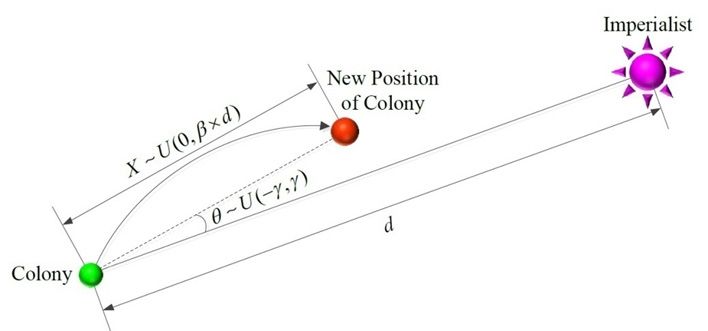

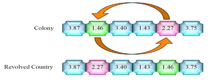
Computer Science and Information Technology 7(4): 103-110, 2019 107

2.3. Moving the Colonies of an Empire toward the solutions of the population size, and then the lowest front
 Imperialist (Assimilating) number is selected if the two populations are from different
 fronts. If they become from the same front, the solution
 After dividing colonies between imperialists, colonies with the highest crowding distance is selected.
are moved toward their related imperialist. This movement
is shown in Figure 3, in which d is the distance between
colony and imperialist. X is a random variable with a 2.5. Revolution
uniform (or any proper) distribution between 0 and β × d In each decade, revolutions are performed on some of
and β is a random number greater than one. Direction of the colonies. For this target, swap operator is selected. The
the movement is shown by θ , which is a random number structures of these operators are described as follows. The
between - γ and γ . revolution rate in this study is shown by Pr.
  Swap: for swapping, two numbers of a colony are first
 selected randomly (numbers 1.46 and 2.27 in Figure
2.4. Information Sharing between Colonies
 4), then the positions of the selected numbers are
 Moreover, colonies are sharing their information exchanged, which is shown in Figure 4.
together by crossover to do themselves better. In this
section, for this target one of these operators including 2.6. Improve Imperialist
one-point, two-point and continuous uniform crossover are
selected randomly. The population percentage that is In this step, the imperialist with minimum power will
sharing information is shown by Pc. The best colonies have generate the maximum neighborhood (Nemax). Likewise,
the more chance than others to share its information the imperialist with the maximum power will generate the
because colonies are selected in this section by the minimum neighborhood (Nemin). The number of
tournament selection, which is described below. A binary neighborhoods associated with each imperialist is
tournament selection procedure has been applied for generated depending on the value of the power and is
selecting solutions for both the crossover and mutation produced using a linear function varying in a range
operators. This procedure works as follow. First select two between Nemin and Nemax, which is shown in Eq. 9.

 Figure 4. Swap operator

 ( Nemax − Nemin )(TP Empworst − TP Empn )
 =Nen floor ( Nemin + ) (9)
 (TP Empworst − TP Empbest )

108 Bi-objective Optimization Model for Integrated Preventive Maintenance and Flexible Job-shop Scheduling Problem

 Where TP Empbest is the value of total power of the
 NTP Empn
strength empire and TP Empworst is the value of total pPn = Nimp
 (11)
power of the weakest power empire. ∑ i =1
 NTP Empi

2.6.1. Colonies Updated Then, the roulette wheel method is used for assigning the
 mentioned colonies to selected empire.
 In each decade, the initial population of colonies,
population of assimilating, population of Information 2.6.5. Eliminating the Powerless Empires
sharing between colonies, population of revolution and Powerless empires will collapse and their colonies will
population of improved imperialist are merged together for be distributed among other empires in the imperialistic
each empire as merged population. Afterward, archived competition. In this paper, when an empire loses all of its
updating is done on merged population. Then, the best of colonies, we consider it collapses.
colonies based on non-dominating sorting and crowding
distance by the population size of colonies for given
empires (NC(i)) are selected for each imperialist. 2.7. Stopping Criteria

2.6.2. Archive Adaption In this paper, the stopping criteria or end of imperialistic
 competition is considered when there is only one empire
 Ranking and sorting is done by the non-dominated and between all of empires. The convergence of the algorithm
crowding distance for the merged population. Then, the in three segments of iterations is illustrated in Figure 5.
solutions of first front are selected in order to add to the
archive. Finally, the solutions of first front are kept and
others are deleted after ranking and sorting solutions in the
archive. Also, the size of archive is equal to nArchive.
2.6.3. Exchanging Positions of the Imperialist and a
 Colony
 First, the total cost of each imperialist is updated. Then,
each imperialist with the best colony are merged together.
Afterward, this population is sorted based on the
non-dominated sorting and crowding distance. Finally, the
best of them is selected as imperialist.
2.6.4. Imperialistic Competition
 
 The power of a weaker empire will reduce, and the
power of more powerful ones will rise in the imperialistic
competition. All empires compete together to take the
position of the weakest colony of the weakest empire. In
other words, first choosing some (usually one) of the
weakest colonies of the weakest empire and then the
position of these colonies (or this colony) are given to the
winner imperialist among all empires in the imperialistic
competition. In this competition, the most powerful

 
empires will not definitely possess these colonies; however,
these empires will be more possible to possess them. This
competition is modeled by just selecting one of the weakest
colonies of the weakest empires and then calculating the
possession probability of empires has the largest
normalized total cost as follows.

NTP Empn max {TP Empi } − TP Empn (10)
=

 Where NTPn is the normalized total power of nth
empire, and TPn is the total power of nth empire. Having
the normalized total power, the possession probability of
each empire is calculated by:
 Figure 5. Convergence of the algorithm

Computer Science and Information Technology 7(4): 103-110, 2019 109

3. Computational Results Table 4. Best, average and worst values of the H metric obtained by
 MOICA

 In this section, some standard flexible job-shop test MOICA
 The number of problems
problems from [3] and [4] are considered. Several standard Best Average Worst
m-machines, n-jobs flexible job-shop test problems are 1 34.72 291.15 607.83
presented. Using the number of jobs (n) and number of
 2 29.46 167.52 503.57
machines (m) noted by couple (n, m), they introduced test
problems with minimum (n,m) of (6, 6) and maximum (n,m) 3 33.09 159.30 347.13
of (30, 10). And for MOICA algorithm two comparison 4 67.62 311.44 829.76
metrics are taken into account. It is noticeable that before 5 29.39 126.16 385.03
calculation of each performance metric, both of objectives 6 48.74 347.94 698.94
are normalized.
 7 61.22 383.01 1267.27
Diversification metric (DM): This metric measure the
spread of the solution set and calculated by: 8 52.86 265.55 1044.35
 9 57.77 391.37 1131.51

 DM = ( max f1i − min f1i )2 + ( max f 2i − min f 2i )2
 (12) 4. Conclusions and Future Studies
 Mean ideal distance (MID): The closeness between
 This paper is developed an integrated model to solve the
Pareto solutions and ideal point ( f1best , f 2best ) is PM and flexible job-shop scheduling problem, and
determined by using the MID. The equation of the MID is optimized two manufacturing systems objectives. Two
defined by: multi-objective evolutionary algorithms were adapted to
 our problem. Computational results with nine standard test
 n
 ( f1i − f1best ) + ( f2i − f2best )
 2 2 problems have shown that the MOICA algorithm provided
 ∑ (13) efficient solutions, based on two performance measures.
 MID = i =1
 As an offer for future studies, it would be considerable to
 n employ other maintenance policies and strategies for this
 Where n is the number of non-dominated solutions and problem.
 fimax min
 ,total and fi ,total are the maximum and minimum
values of each fitness functions among the all
non-dominated solutions obtained by the algorithms,
respectively. Table 2 represents the best, average and worst REFERENCES
number of obtained solutions. Table 3 gives the best, the
average and the worst value of the C metric obtained over Berrichi, A., Amodeo, L., Yalaoui, F., Châtelet, E., &
the solution sets. Table 4 illuminates the H metric obtained Mezghiche, M., 2008. Bi-objective optimization
 algorithms for joint production and maintenance
over solution sets. scheduling: Application to the parallel machine problem.
 Journal of Intelligent.
Table 3. Best, average and worst values of the C metric obtained by
MOICA
 E. Moradi, S.M.T. Fatemi Ghomi, M. Zandieh., 2011.
 MOICA Bi-objective optimization research on integrated fixed
 The number of problems time interval preventive maintenance and production for
 Best Average Worst scheduling flexible job-shop problem. Expert Systems
 1 1 0.29 0 with Applications, 38, 7169-7178.
 2 0.89 0.32 0 E. Atashpaz-Gargari and C. Lucas, Imperialist
 3 1 0.24 0 competitive algorithm: An algorithm for optimization
 inspired by imperialist competitive. IEEE Congress on
 4 1 0.36 0 Evolutionary computation, Singapore, 2007.
 5 1 0.38 0
 Ishibuchi, H., Yoshida, T., & Murata, T., 2003. Balance
 6 1 0.30 0 between genetic search and local search in memetic
 7 0.76 0.26 0 algorithms for multi-objective permutation flow-shop
 scheduling. IEEE Transactions on Evolutionary
 8 1 0.44 0 Computation, 7(2), 204-223.
 9 1 0.31 0

110 Bi-objective Optimization Model for Integrated Preventive Maintenance and Flexible Job-shop Scheduling Problem

 Kaabi, J., Varnier, C., & Zerhouni, N., 2003. Genetic
 algorithm for scheduling production and maintenance in
 a flow-shop. France: Laboratory of Automatic of
 Besancon. In French.
 Sioud A.G.M. and Cagne, C., 2012. A hybrid genetic
 algorithm for a single machine scheduling problem with
 sequence dependent setup times. Computers and
 Operations Research, 39, 2415-2424.