BOBMEX: The Bay of Bengal Monsoon Experiment
←
→
Page content transcription
If your browser does not render page correctly, please read the page content below
BOBMEX: The Bay of Bengal
                             Monsoon Experiment
               G. S. Bhat,* S. Gadgil,* P. V. Hareesh Kumar,+ S. R. Kalsi,# P. Madhusoodanan,+
                       V. S. N. Murty,@ C. V. K. Prasada Rao,+ V. Ramesh Babu,@ L. V. G. Rao,@
                                R. R. Rao,+ M. Ravichandran,& K. G. Reddy,** P. Sanjeeva Rao,++
                             D. Sengupta,* D. R. Sikka,## J. Swain,+ and P. N. Vinayachandran*

      ABSTRACT

           The first observational experiment under the Indian Climate Research Programme, called the Bay of Bengal Mon-
      soon Experiment (BOBMEX), was carried out during July–August 1999. BOBMEX was aimed at measurements of
      important variables of the atmosphere, ocean, and their interface to gain deeper insight into some of the processes that
      govern the variability of organized convection over the bay. Simultaneous time series observations were carried out in
      the northern and southern Bay of Bengal from ships and moored buoys. About 80 scientists from 15 different institu-
      tions in India collaborated during BOBMEX to make observations in most-hostile conditions of the raging monsoon.
      In this paper, the objectives and the design of BOBMEX are described and some initial results presented.
           During the BOBMEX field phase there were several active spells of convection over the bay, separated by weak
      spells. Observation with high-resolution radiosondes, launched for the first time over the northern bay, showed that
      the magnitudes of the convective available potential energy (CAPE) and the convective inhibition energy were com-
      parable to those for the atmosphere over the west Pacific warm pool. CAPE decreased by 2–3 kJ kg−1 following con-
      vection, and recovered in a time period of 1–2 days. The surface wind speed was generally higher than 8 m s−1.
           The thermohaline structure as well as its time evolution during the BOBMEX field phase were found to be different
      in the northern bay than in the southern bay. Over both the regions, the SST decreased during rain events and in-
      creased in cloud-free conditions. Over the season as a whole, the upper-layer salinity decreased for the north bay and
      increased for the south bay. The variation in SST during 1999 was found to be of smaller amplitude than in 1998.
      Further analysis of the surface fluxes and currents is expected to give insight into the nature of coupling.

1. Introduction                                                    variability of the Indian monsoon is, therefore, ex-
                                                                   tremely important for the well-being of over one bil-
   The monsoon governs the very pulse of life on the               lion people and the diverse fauna and flora inhabiting
Indian subcontinent. Understanding and predicting the              the region. The major thrust of the Indian Climate
                                                                   Research Programme (ICRP) is on monsoon variabil-
                                                                   ity, on timescales ranging from subseasonal to
*Indian Institute of Science, Bangalore, India.                    interannual and decadal, and its impact on critical re-
+
  Naval Physical and Oceanographic Laboratory, Kochi, India.       sources (DST 1996). The monsoon is strongly coupled
#
  India Meteorological Department, New Delhi, India.               to the warm oceans surrounding the subcontinent.
@
   National Institute of Oceanography, Goa, India.                 Most of the monsoon rainfall occurs in association
&
  National Institute of Ocean Technology, Chennai, India.
**Department of Meteorology and Oceanography, Andhra Uni-
                                                                   with synoptic-scale systems, that is, the monsoon dis-
versity, Visakhapatnam, India.                                     turbances, which are generated over these waters and
++
   Department of Science and Technology, New Delhi, India.         move onto the Indian landmass (e.g., Fig. 1a for the
##
   Mausam Vihar, New Delhi, India.                                 monsoon season of 1999). In particular, the Bay of
Corresponding author address: Sulochana Gadgil, Centre for         Bengal (hereafter called the bay) is exceptionally fer-
Atmospheric and Oceanic Sciences, Indian Institute of Science,
                                                                   tile, with a very high frequency of genesis of these
Bangalore 560 012, India.
E-mail: sulo@caos.iisc.ernet.in                                    systems (Rao 1976).
In final form 15 March 2001.                                           The distribution of the summer monsoon (Jun–
©2001 American Meteorological Society                              Sep) rainfall over the Indian region is linked to the

Bulletin of the American Meteorological Society                                                                              2217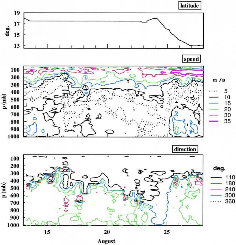
(a) variation of the convection over the bay (Gadgil 2000).
For example, during the summer monsoon of 1998, the
convection over the northern bay was anomalously
low, with occurrence of relatively few systems,
whereas a large number of systems formed over the
southern parts of the bay. Thus the anomalies of the
outgoing longwave radiation (OLR) were positive
over the northern bay and negative over the southern
bay (e.g., Fig. 1b for Jul 1998). Most of these systems
moved from the southern bay onto and across the
southern peninsula. The rainfall anomalies were, there-
fore, positive over the southern peninsula. Large defi-
cits occurred in the north, particularly over the east
coast of India, adjacent to the northern parts of the bay
(e.g., Fig. 1b). The 1998 season was not an exceptional
one in the distribution of rainfall anomalies over the
Indian region; in fact, a similar pattern occurred in 2000.
Summer monsoon rainfall over the Indian region
exhibits strong variability on intraseasonal timescales
involving a 10–20-day westward propagating mode
(Krishnamurti and Bhalme 1976; Krishnamurti and
(b) Ardunay 1980) and a 30–50-day northward propagat-
ing mode (Sikka and Gadgil 1980; Yasunari 1981).
The northward propagations over the bay are clearly
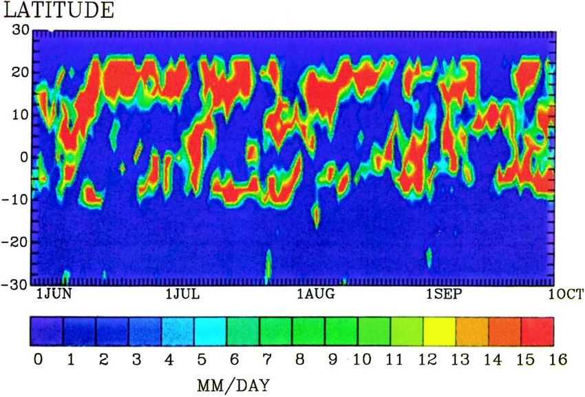
seen in Fig. 2, which depicts the variation of micro-
wave sounding unit (MSU) precipitation during the
summer of 1986. The major subseasonal variation of
the monsoon rainfall can be viewed as alternating
active spells and weak spells or breaks (Fig. 3). Active
spells are characterized by high frequency of genesis
of synoptic-scale systems over the bay, which propa-
gate onto and produce widespread rainfall on the sub-
continent; whereas there is a paucity of synoptic
systems over central India during a break spell of the
monsoon. Revival of the Indian rainfall from mon-
soon breaks occurs either with the westward propa-
gation of a disturbance generated over the north bay
(in association with the 10–20-day mode) or north-
ward propagation of the tropical convergence zone
(TCZ) generated over the equatorial Indian Ocean
across the bay and Arabian Sea (in association with
the 30–50-day Madden–Julian mode). Thus, convec-
FIG. 1. (a) Tracks of monsoon lows and depressions for the tion over the bay plays an important role in the varia-
monsoon season of 1999. Monsoon lows and depressions are syn- tion of synoptic-scale systems as well as in the
optic-scale systems and identified in a surface pressure chart by intraseasonal variation in which these systems are
one, and two to three closed contours (at 2-mb interval), respec- embedded. Interannual variation of the monsoon is
tively. (b) OLR anomalies (W m−2) over the Bay of Bengal and
rainfall anomalies (% of average) over the Indian subcontinent
strongly linked to the intraseasonal variation, with
during Jul 1998. Deficit convection (positive OLR anomalies) poor monsoon seasons characterized by long breaks
over the ocean and deficit rainfall (negative rainfall anomalies) (e.g., Fig. 3). Clearly, for understanding variations of
over land are marked by red, and greenish yellow refers to nor- the monsoon over the Indian subcontinent on
mal or above normal convection/precipitation. intraseasonal as well as interannual timescales, it is
2218 Vol. 82, No. 10, October 2001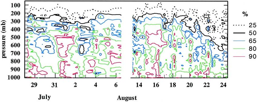
FIG. 2. Variation of rainfall measured by MSU over the 90°–92.5°E longitudinal belt during the summer monsoon of 1986.
(Courtesy J. Srinivasan.)

important to understand processes that determine the          SST changes in these phases appear to be largely due
variability of organized convection over the bay.             to a direct response to the changes in net heat flux.
    The intraseasonal variation over the bay is clearly           Earlier studies suggest that atmospheric conditions
brought out in the observed SST and wind speed from           have a significant impact on the SST of the bay.
a moored buoy and Indian National Satellite System            However, the extent to which variation of SST modu-
(INSAT) OLR (outgoing longwave radiation) data                lates the convection over the bay is not known. The
during July–August 1998 (Fig. 4). It is seen that the         problem is complex because the SST of the bay is
dominant timescale of variation of OLR, wind speed,           above the convection threshold of 27.5°C (Gadgil et al.
and SST is intraseasonal, with the maxima–minima              1984; Graham and Barnett 1987) throughout the sum-
separated by about 1 month. During this 2-month               mer. Understanding the nature of the feedbacks be-
period, three spells of low OLR were observed. The            tween the atmospheric convection and surface
amplitude of variation of SST can be about 2°C in the         conditions of the bay is important for understanding
north bay (Fig. 4a). The amplitude and timescales of          the variability of convection over the bay. A major in-
variation in SST appear to be comparable to those in          ternational program, the Tropical Ocean Global Atmo-
the equatorial west Pacific Ocean (Anderson et al.            sphere Coupled Ocean–Atmosphere Response
1996). The phases with decreasing (increasing) OLR            Experiment (TOGA COARE), aimed at elucidating
are generally associated with decreasing (increasing)         the coupling of the west Pacific warm pool to the at-
SST, with changes in OLR leading those in SST by a            mosphere (Webster and Lukas 1992), has given con-
few days. Sengupta and Ravichandran’s (2001) study            siderable insight into ocean–atmosphere coupling on
has shown that the net heat flux into the ocean is nega-      intraseasonal timescales (Godfrey et al. 1998; Shinoda
tive in the active phase of convection and positive in        et al. 1998). However, there are important differences
the weak phase of convection in the bay; the observed         between the thermohaline structure of the bay and the

Bulletin of the American Meteorological Society                                                                   2219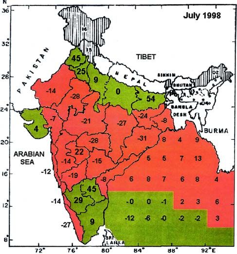
FIG. 3. Daily rainfall over central India during 1972 and 1975, which were deficit and excess monsoon rainfall years, respectively.
In 1972, active and weak rain spells were well separated with the break during the last week of Jul and first week of Aug clearly seen,
whereas in 1975, although there were days of heavy rainfall (active spell), there were no clear-cut breaks.

west Pacific (Varkey et al. 1996) as well as in the at-              forcing over these two regions. Over the west Pacific
mospheric forcing over these two regions. During the                 the winds are light, only occasionally exceeding
summer monsoon season, the bay receives a large                      4 m s−1 (Weller and Anderson 1996), whereas over the
amount of freshwater from rain. The north bay also                   bay they are much stronger during the monsoon, of-
receives a comparable amount of freshwater from river                ten greater than 8 m s−1. Also, the amplitude of SST
runoff (Shetye and Gouveia 1998). As a result, the                   variation on a 30–90-day Madden–Julian oscillation
near-surface layer (0–30 m) of the north bay has rela-               timescale is weak and about 0.15°C over the Indian
tively fresh water throughout the summer (Murty et al.               Ocean compared to about 0.25°C over the west Pa-
1992, 1996; Sprintall and Tomczak 1992). Over the                    cific (Shinoda et al. 1998). Perhaps the intraseasonal
west Pacific, a near-surface layer of relatively fresh               oscillations shorter than the 30-day timescale are more
water, with a barrier layer beneath, appears intermit-               important in the Indian Ocean. This points to the need
tently (Godfrey and Lindstrom 1989; Lukas and                        of a special observational experiment over the bay for
Lindstrom 1991). Further, the salinity gradient be-                  understanding the nature of the coupling between the
tween the surface layer of the west Pacific and the                  atmosphere and the ocean.
ocean below is much smaller than that over the bay.                      Under the ICRP, a special observational program
There are important differences in the atmospheric                   called the Bay of Bengal Monsoon Experiment

2220                                                                                              Vol. 82, No. 10, October 2001
(BOBMEX) was conducted during July–August                   (a)
1999. BOBMEX was aimed at collecting critical data
on the subseasonal variation of important variables
of the atmosphere, ocean, and their interface to gain
deeper insight into some of the processes that govern
the variability of organized convection over the bay
and its impact. About 80 scientists from 15 different
institutions in India collaborated during BOBMEX to
make observations in the hostile conditions of the
monsoon. This paper is written with a view to intro-
ducing BOBMEX to the international scientific com-
munity and presenting a few initial results. Several
questions raised by the preliminary analysis of
BOBMEX data are being addressed at present with
detailed investigations. We expect BOBMEX obser-
vations to complement the observations from the pi-
lot study for the Joint Air–Sea Monsoon Interaction
Experiment carried out in the southern Bay of Ben-
gal during May–June and September 1999 (Webster
et al. 2000, manuscript submitted to Bull. Amer.
Meteor. Soc.).
    We briefly discuss the background in the next sec-
tion, and the scientific objectives and the design of the
experiment in section 3. In section 4, the sensors,
instruments, and the observations during the inter-
comparison experiments are briefly described. We
                                                            (b)
consider the general features of the variation of con-
vection and the surface variables over the bay during
BOBMEX in section 5. Some results from the obser-
vations of the atmosphere and ocean are presented in
sections 6 and 7, respectively, and concluding remarks
in section 8.

2. Background

a. Earlier observational experiments
    Two major international observational experiments
were conducted over the bay in the 1970s, namely,
MONSOON-77 and MONEX-79. MONSOON-77
involved four Soviet Union (USSR) ships forming a
polygon over the bay centered at 17°N, 89°E during
11–19 August 1977. A trough formed in the north bay
on 16 August and developed into a depression on                FIG. 4. Variation of INSAT OLR and SST from moored buoys
19 August. During MONEX-79 (Fein and Kuettner               during Jul–Aug 1998 (after Premkumar et al. 2000). (a) North bay
                                                            (18°N, 88°E). Wind speed (3-m height) from the buoy is also
1980), four USSR ships and upper ocean current meter        shown. (b) South bay (13°N, 87°E).
moorings formed a stationary polygon centered at
16.2°N, 89.5°E during 11–24 July 1979. In addition,
data were collected with dropwindsondes from                tions could not be studied. Apart from these two ma-
aircrafts. This period happened to be a weak phase of       jor experiments, observations from a ship were made
convection over the bay, and hence disturbed condi-         at 20°N, 89°E during 18–31 August and 9–19 Sep-

Bulletin of the American Meteorological Society                                                                      2221
tember 1990, coinciding with the Monsoon Trough Variation of convection in the atmosphere depends
Boundary Layer Experiment (MONTBLEX-90) car- upon dynamics as well as thermodynamics. There is
ried out over the northern plains of the Indian subcon- considerable understanding of the structure and dy-
tinent (Goel and Srivastava 1990). namics of the synoptic-scale systems over the bay
The differences in the horizontal wind fields, ver- (e.g., Rao 1976; Sikka 1977). However, there have not
tical velocity, and large-scale heat and moisture bud- been many detailed observations of the vertical struc-
gets between disturbed and undisturbed conditions in ture of the atmosphere over the bay using high-
the bay were studied by analysis of these data (e.g., resolution radiosondes. Hence, the variation in the
Mohanty and Das 1986). Studies based on the data stability of the atmosphere and its links with variation
from these experiments suggest that the genesis of the in convection are yet to be elucidated. We expect feed-
synoptic-scale systems occurs over regions of the bay backs between convection and the thermodynamics to
with high SST and high heat content in the surface play an important role in determining variation of con-
layer (Rao et al. 1987; Sanil Kumar et al. 1994). The vection (Emanuel 1994, chapter 15). A critical param-
impact of the synoptic-scale systems on the ocean be- eter for atmospheric convection is the convective
neath was found to be a decrease in SST that can be available potential energy (CAPE), a measure of the
as large as 2°–3°C for the most intense systems (Rao vertical instability of the atmosphere under moist con-
1987; Gopalakrishnan et al. 1993). Observations dur- vection (Moncrief and Miller 1976). CAPE is the work
ing MONTBLEX-90 indicated that SST decreased by done by the buoyancy force on a parcel lifted through
0.2°–0.3°C for weaker systems (Murty et al. 1996; the atmosphere moist adiabatically and is given by
Sarma et al. 1997). The SST increases after the sys- (e.g., Williams and Renno 1993)
tem attenuates or moves away. The timescale for this
recovery was about a week for the systems observed LNB
during MONEX-79 (Rao 1987; Gopalakrishna et al.
1993).
CAPE = − ∫ (T
LFC
vp )
− Tve RD d (ln p), (1)
b. New observations required where RD is the gas constant of dry air; Tvp and Tve,
Previous observational experiments (MONEX-79, are, respectively, the virtual temperatures of the par-
in particular) have contributed to our knowledge of the cel and the environment at pressure p; and LFC and
large-scale features of the Indian summer monsoon LNB are levels of free convection and neutral buoy-
(Krishnamurti 1985). However, detailed observations ancy, respectively. Deep clouds can develop by the
for studying the vertical structure of the atmosphere, ascent of air from a given level only if its CAPE is
ocean, and their interface during all phases of convec- greater than zero. When disturbances occur, precipi-
tion were not available for the bay. Further, all tation, strong winds, and downdrafts decrease the en-
components of the surface fluxes have not been di- ergy of the air near the surface, while deep cloud
rectly measured over the north bay previously. activity makes the upper troposphere warmer. As a
Accurate measurements of surface fluxes over the result, the atmosphere becomes less unstable and
west Pacific have led to realistic simulations of SST CAPE is substantially reduced during disturbances
with ocean mixed layer models (Anderson et al. 1996). (Emanuel 1994, chapter 15). When disturbances at-
The summer mean surface salinity in the north bay is tenuate, the air–sea fluxes increase the energy of the
very low (Levitus and Boyer 1994) and SSTs are high. surface air, while the temperature of the air aloft de-
It is likely that the high upper ocean stability in this creases because of radiative cooling. These factors
region (Rao et al. 1993) is responsible for the persis- destabilize the atmosphere and build up CAPE. The
tent high SST. The upper ocean processes in the pres- period between successive disturbances is expected to
ence of strong monsoonal winds and low surface depend upon the time it takes for the CAPE to build
salinity need to be understood. Therefore, it is impor- up. How the instability builds up, the changes that take
tant to measure heat and freshwater fluxes over the bay place with the growth/arrival of monsoon distur-
with sufficient accuracy, along with upper ocean tem- bances, how much instability is consumed, and the
perature and salinity profiles. Within the bay, there manner in which it recovers after the disturbance are
are marked variations in the freshwater flux between the basic issues that are yet be understood for the bay.
the northern and southern parts. Hence, measurements It is also important to understand if there are any criti-
of fluxes in each of these regions are required. cal values of the height of the atmospheric boundary
2222 Vol. 82, No. 10, October 2001layer and air properties (such as moist static energy (a)
and equivalent potential temperature) vis-à-vis the
thermal stratification of the atmosphere above, for the
onset of convection.
Normally air is not saturated to start with and a fi-
nite vertical displacement (a few hundred meters to a
few kilometers) is needed for the rising air parcel to
become saturated and reach the level of free convec-
tion. Some energy is required for this process, and is
called convection inhibition energy [CINE, after Wil-
liams and Renno (1993)]. CINE is calculated from the
integral (Williams and Renno 1993)
LFC
CINE = ∫ (T
pi
vp )
− Tve RD d (ln p), (2)
where pi is the parcel’s starting pressure level. It is
expected that a larger value of CINE means an in-
creased barrier to convection. If CINE is large, deep
clouds will not develop even if CAPE is positive. (b)
While low values of CINE imply a favorable condi-
tion for convection, the critical value of CINE above
which convection cannot occur has not been estab-
lished. For the estimation of CAPE and CINE, tem-
perature and humidity data with high vertical
resolution are required. Such data were not available
for the atmosphere over the north bay, prior to
BOBMEX.
3. Scientific objectives and design of the
experiment FIG. 5. (a) Cruise tracks, time series observation stations (TS1
and TS2), and buoy locations (DS3 and DS4) in the Bay of Ben-
gal during BOBMEX. Period: 16 Jul–30 Aug 1999. SK, RV Sagar
A study of the impact of convection on the ocean, Kanya; SD, INS Sagardhwani. Observation positions: TS1, 13°N,
the recovery/changes after the convection attenuates 87°E; TS2, 17.5°N, 89°E; DS3, 13°N, 87°E; and DS4, 18°N,
and/or moves away, and the characteristics during 88°E. (b) The RV Sagar Kanya. The boom and manual surface
calm phases when convection is absent for several meteorological observation (metkit) positions are indicated.
days was envisaged. The emphasis of BOBMEX was
on collecting high quality data during different phases Experiment design
of convection over the bay, which can give insight into In this first major Indian experiment, it was not
the nature of coupling between the convective systems possible to deploy as large a number of observation
and the bay. platforms as we would have liked. The two deep
In brief, the scientific objectives of BOBMEX moored buoys that provided valuable data during the
were to document and understand, during different monsoon of 1998 were stolen a few months before the
phases of convection, the variations of (i) the vertical experiment. Since buoy data are a critical component
stability of the atmosphere and the structure of the at- of BOBMEX, new buoys were installed in the north-
mospheric boundary layer, (ii) fluxes at the surfaces ern and southern bay (henceforth referred to as DS4
of the ocean, and (iii) the thermohaline structure and and DS3, respectively) during the initial phase of
the upper ocean currents. BOBMEX (Fig. 5a). In addition, RV Sagar Kanya
(SK), a research vessel belonging to the Department of
Bulletin of the American Meteorological Society 2223Ocean Development, and INS Sagardhwani (SD), of chosen to be close to the buoys so that reliability of
the Naval Physical and Oceanographic Laboratory of the observations from two independent platforms
the Defence Research and Development Organisation, could also be assessed. The cruise tracks of the two
were deployed. The India Meteorological Department ships and buoy locations are also shown in Fig. 5a.
organized special observations from coastal and island In addition to the observations at stationary positions
stations. in the northern and southern bay, observations were
The timescales of intraseasonal variation are of the made along zonal sections when the ships made port
order of 3–4 weeks for the bay (Fig. 4). The time se- calls (at Paradip and Chennai) and north–south sec-
ries from the earlier observational experiments were tions at the beginning and the end of the experiment
too short to reveal variations on these supersynoptic (Fig. 5a).
scales. Hence, it was decided to aim for time series Measurements of all components of surface fluxes,
observations for about 6 weeks. Two locations—one including radiation; the vertical profiles of atmo-
each in the southern and northern bay—were chosen spheric temperature, humidity, and winds; and ocean
for the time series observations (henceforth referred temperature, salinity, and current profiles were
to as TS1 and TS2, respectively; see Fig. 5a). The planned from both the ships.
choice of these two locations was based on the follow-
ing consideration. The occurrence of organized con-
vection is high at both the locations. During the 4. Sensors, instruments, and
northward propagation of the tropical convergence intercomparison
zone the systems tend to move across the bay from
south to the north (Sikka and Gadgil 1980). Therefore, The basic surface meteorological variables mea-
it is important to document the gradients in atmo- sured were wind (speed and direction), temperature
spheric variables and SST between these two regions. (dry bulb, wet bulb, and sea surface), humidity, pres-
Also, there are marked differences in the freshwater sure, radiation, and precipitation. In order to calculate
fluxes at these two locations and hence in the thermo- the fluxes by direct methods, wind velocity, tempera-
haline structure of the upper layers of the ocean. The ture, humidity, and ship acceleration and tilt were
differences, if any, in the response of the ocean to con- measured using fast response sensors at 10 Hz. The
vection at these locations could provide further insight major meteorological sensors and instruments used on
into coupling. In fact, the choice of the location of the the ships and buoys are listed in Table 1. The loca-
buoys was based on a similar rationale. The locations tion of the boom and manual (metkit) observation po-
of the research ships for time series observations were sition on the Research Vessel SK are shown in Fig. 5b.
TABLE 1. Major meteorological sensors/instruments operated during BOBMEX.
Plat- Averaging Sampling
Parameter form Sensor/instrument Locationa Make Accuracy time interval
b
Hand-held cup Deck (~14 m) Ogawaseiki, Japan — 3h
SK anemometer
(metkit),
sonic anemometer, Boom (~11.5 m) Metek, Germany 0.1 m s−1 1 min Continuous, 0.1 Hz
−1
Wind Gill anemometer Boom (~11.5 m) R. M. Young, U.S.A. 0.2 m s 1 min Continuous, 0.1 Hz
b
SD Hand-held Deck (~10 m) — — 3h
cup anemometer
DS3 Cup anemometer Tower (3 m) Lambrecht 1.5% FS 10 minc 3h
a
Numbers inside the parentheses are approximate heights above the sea surface.
b
The hand-held instruments were typically exposed for 3 min.
c
From samples collected at 1 Hz.
2224 Vol. 82, No. 10, October 2001TABLE 1. (Continued.)
Plat- Averaging Sampling
Parameter form Sensor/instrument Locationa Make Accuracy time interval
b
Hg in glass Deck (~14 m) — 0.25°C 3h
thermometer
SK (metkit),
Sonic anemometer, Boom (11.5 m) Metek 0.1°C 1 min Continuous, 0.1 Hz
Platinum resistance Boom (11.5 m) R. M. Young 0.3°C 1 min Continuous, 1 Hz
Temperature thermometer
SD Metkit, Hg in Deck — 0.5°C 3h
glass thermometer
DS3 Platinum resistance Tower (3 m) Omega Eng. 0.1°C 10 minc 3h
thermometer
Pressure SK Pressure gauge Met lab — 0.5 hPa — 3h
SD Pressure gauge Met lab — 0.5 hPa — 3h
DS3 Capacitor film — Vaisala 0.1 hPa — 3h
Psychrometer Deck (14 m) IMD — — 3h
SK Humicap Boom (11.5 m) R. M. Young 2% 1 min Continuous, 1 Hz
Relative IR hygrometer Boom (11.5 m) Applied Technology 0.5 gm m−3 1 min Continuous, 0.1 Hz
humidity
SD Psychrometer Deck (11.5 m) — — — 3h
SK Automatic rain Open space R. M. Young 1 mm 1 min Continuous, 1 Hz
Precipitation gauge
SD Automatic rain Open space R. M. Young 1 mm 1 min Continuous, 1 Hz
gauge
Acceleration SK Three-axis Sonic Crossbow 0.05 m s−2 0.1 s Continuous, 0.1 Hz
tilt accelerometer anemometer Technology Inc.
SK Two-axis tiltmeter Sonic Crossbow 0.5° 0.1 s Continuous, 0.1 Hz
anemometer Technology Inc.
Global SK Spectral Gymbal Eppley, U.S.A. 1 min Continuous, 1 Hz
solar pyranometer (incoming) ~10 W m−2
radiation Boom Eppley 1 min Continuous, 1 Hz
(incoming) (outgoing)
and outgoing)
SD Pyranometer Boom/deck Kipp and Zonen ~10 W m−2 5 min Continuous
Global IR radiometer Gymbal Eppley 1 min Continuous, 1 Hz
longwave SK (incoming) ~10 W m−2
radiation
Boom (outgoing) Eppley 1 min Continuous, 1 Hz
(incoming
and outgoing) SD Pyrgeometer Boom/deck Kipp and Zonen ±10% 5 min Continuous
a
Numbers inside the parentheses are approximate heights above the sea surface.
b
The hand-held instruments were typically exposed for 3 min.
c
From samples collected at 1 Hz.
Bulletin of the American Meteorological Society 2225The boom was a 7-m-long horizontal shaft with pro- water samples for dissolved oxygen, nutrients,
visions to fix sensors. Measurement of the vertical pro- dimethylsulfide, and nitrous oxide were carried out.
files of temperature, humidity, and wind were possible The results of the analysis of atmospheric–oceanic
only from SK. In addition, atmospheric ozone and chemistry will be presented separately.
aerosol concentrations have been measured by the sci- BOBMEX envisaged the use of a large number of
entists from the Indian Institute of Tropical Meteo- state-of-the-art sensors and instruments, some of them
rology, in Pune. The basic oceanographic variables used for the first time on an Indian research ship. In
measured include current, temperature, salinity, wave order to test the new sensors acquired for BOBMEX
height and period, chlorophyll, and light transmission. and to evolve strategies for coordination among dif-
The major oceanographic sensors and instruments ferent agencies, data quality control, acquisition, ar-
used are given in Table 2. Chemical analysis of the chival, dissemination, and analysis, a pilot experiment
TABLE 2. Major oceanographic instruments used during BOBMEX.
Plat- Sampling
Parameter form Sensor/instrument Make/model Range Accuracy Resolution Interval
Water SK CTD SBE model 911 −5° to 35°C ±0.01°C 0.0002°C 3h
column plus
temperature
SD Mini-CTD SD 204 −2° to 40°C ±0.01°C 0.005°C 3h
Water SK CTD SBE model 911 0–7a ±0.0003a 0.00004a 3h
column plus
conductivity SD Mini-CTD SD 204 0–7a ±0.002a 0.001a 3h
SK CTD — Up to 6800-m ±0.015%b 0.001%b 3h
Pressure depth
SD Mini-CTD — Up to 500-m ±0.02%b 0.01%b 3h
depth
SK VM-ADCP RD Instruments 250 mc ±1 cm s−1 0.01 cm s−1, 0.2° 10 min
Horizontal
SD VM-ADCP RD Instruments 250 m c
± 1 cm s −1
10 min
current
−1
DS3 Acoustic UCM60 — 1 cm s 3h
Doppler
SK SWRd — — —
Wave SD SWR — — —
DS3 Accelerometer MRV-6 — 10 cm
and compass
SK Bucket T. F. and Co., −13° to 42.5°C 0.25°C — 3h
thermometer, Germany
SST SD bucket — — 0.5°C — 3h
thermometer,
DS3 Platinum resistance UCM-60 −5° to 45°C 0.1°C — 3h
thermometer
a
Siemens−1.
b
Percent of full scale.
c
Maximum profiling range.
d
Shipborne wave recorder.
2226 Vol. 82, No. 10, October 2001was carried out during October–November 1998 in the water column temperatures measured by CTDs from
southern bay on board SK (Sikka and Sanjeeva Rao ships, especially in the mixed layer and in the upper
2000). Preliminary results have been published (e.g., thermocline. There is also broad agreement in the sa-
Bhat et al. 2000; Ramesh Babu et al. 2000) and fur- linity data, which improved after subjecting the SD
ther analysis of these data is being carried out. salinity data to spike removal and other standard qual-
Considerable efforts have been made to ensure that ity control operations.
high quality data are obtained in BOBMEX. The se- Also, data from different instruments measuring
lection of the sensors/instruments for the surface ob- the same variable on the ship have been intercompared.
servations, wherever possible, was made considering For example, in Fig. 6b the air temperature (Ta ), spe-
the Improved Meteorology (IMET) system developed cific humidity (qa), and horizontal wind speed (U) are
by the Woods Hole Oceanographic Institution for ap- compared. The data for the sensors mounted on the
plication in the marine environment (Hosom et al. boom and shown in Fig. 6b are 10-min averages cal-
1995). The makes of the sensors used for wind, pre- culated from the continuous data sampled at 10 Hz for
cipitation, and radiation measurements (Table 1) in- the sonic anemometer, Gill anemometer, and IR hy-
cluded those selected for the IMET system. The grometer, and 1 Hz for the PRT and humicap sensors
relative humidity (humicap) and platinum resistance (Table 1). The metkit data are typically 2–3-min av-
thermometer (PRT) sensors were calibrated in the erages. The metkit wind speed has been reduced to
laboratory before and after the field experiment us- 11.5-m height (mean height of wind sensors on the
ing the same cables as those used on the ship. The ra- boom) using the Monin–Obukhov similarity profiles
diation instruments were compared with the standards (Liu et al. 1979). Observed mean and rms differences
at the Central Radiation Laboratory, India Meteoro- for the period are shown in Table 3. The sonic an-
logical Department at Pune, and were found to main- emometer measures the virtual temperature (Tv ), while
tain their original sensitivities. The Gill anemometer the humicap measures the relative humidity (RH). Air
and sonic anemometer were tested in the wind tunnel temperatures from sonic anemometer data and specific
at the Indian Institute of Science in the 4–15 m s−1 humidity from humicap data are obtained by iteration.
wind speed range and were found to be in excellent It is observed from Fig. 6b that air temperatures
agreement with the wind tunnel data and with each measured from PRT, sonic anemometer, and metkit
other. are in broad agreement with each other. The metkit
Further, intercomparison experiments were carried temperature shows a large diurnal amplitude compared
out at the TS1 location for about a 12-h duration at to PRT and sonic temperatures, reflecting the partial
the start and end of the BOBMEX field phase to as- effect of the ship deck (which responds more quickly
sess the relative accuracies of the data collected on two to radiative heating/cooling) on the metkit tempera-
ships and buoy DS3. The data from intercomparison ture. PRT temperature shows a slightly larger diurnal
experiments showed consistency and good agreement variation (on 22 and 23 Aug, in particular) compared
between observations made from DS3, SK, and SD to the sonic anemometer air temperature. Perhaps this
(ICRP 2000). For example, Fig. 6a shows SST, wind is due to the influence of the radiation shield inside
speed, and water column temperature and salinity which the PRT was placed. Good agreement is ob-
measured from the ships and the buoy on 27 August served for the specific humidity also. Calibrations
at TS1. SSTs shown are bucket SSTs for the ships using the standard salt solutions confirmed that the
(measured about 1 m below the surface) and those of humicap RH is accurate within 2% in the 70%–90%
the buoy are from a platinum resistance thermometer RH range. This corresponds to about 0.5 gm kg−1 un-
placed 3 m below the surface. The maximum differ- certainty in the mixing ratio. IR hygrometer and
ence in SSTs is 0.4°C, with the average difference be- humicap data are within this range for the majority of
ing less than 0.25°C, the reading accuracy of the the time. Sudden increases in IR hygrometer humid-
bucket thermometer. Wind speeds (reduced at 10-m ity are occasionally seen. The IR hygrometer is based
height using Monin–Obukhov similarity profiles) on the principle of absorption of infrared radiation by
agreed with each other within 1 m s−1 . The turbulent the water vapor in a small volume of air. Its readings
nature of the wind and the spatial separation (ships and are not accurate when water droplets are present in the
the buoy were 5–15 km apart owing to safety consid- sampling volume, for example, when it was raining
erations) contributed to the differences, as did instru- on 20 and 22 August. If such periods are not consid-
ment differences. There is good agreement between the ered, then the mean difference between the humicap
Bulletin of the American Meteorological Society 2227FIG. 6a. Comparison of SST (top) and wind speed (middle) measured from SK, SD, and DS3 on 27 Aug 1999 (IST: Indian standard time.) The wind speeds shown are calculated at 10-m height using Monin–Obukhov similarity profiles. SST on DS3 was measured at 3-m depth, and from SK and SD around 1-m depth. (bottom) Ocean temperature and salinity profiles measured from SK and SD. and IR hygrometer specific humidities is 0.1 gm kg−1 by the sonic and Gill anemometers (average and rms and the rms difference is 0.3 gm kg−1 (Table 3). The differences are 0.1 and 0.3 m s −1, respectively; metkit mixing ratio is also in good agreement with the Table 3). The metkit wind speed is 1 m s−1 larger in humicap data. There is excellent agreement between the mean. This difference is probably due to the ac- the wind speeds (corrected for the ship drift) measured celeration of the air caused by the ship structures that 2228 Vol. 82, No. 10, October 2001
tervals varying between 5 and 9 days. The duration
                                                                    of each of these spells varies from 2 to 5 days. Between
                                                                    these active spells there are spells with almost cloud-
                                                                    free conditions, that is, with high OLR, which last for
                                                                    2–7 days. As in 1998, the phases of decreasing (in-
                                                                    creasing) OLR are generally associated with decreas-
                                                                    ing (increasing) SST. The exception is the period
                                                                    6–9 August, in which SST hardly changed, although
                                                                    there were large variations in OLR. This is similar to
                                                                    the event during 1–7 August in 1998 (Fig. 4b) in
                                                                    which the SST remained relatively steady. We return
                                                                    to a discussion of these events later in this section.
                                                                    Also note that the amplitude of variation of the SST
                                                                    in 1999 is much smaller than that in 1998. An impor-
                                                                    tant question to address in future studies is understand-
                                                                    ing why there was such a large difference in SST
                                                                    variations between the two monsoon seasons over the
                                                                    bay.
                                                                        In active spell I (Fig. 7a), a low pressure system
                                                                    was generated in the north bay on 25 July, intensified
   FIG. 6b. Comparison of air temperature, specific humidity, and   into a depression on 27 July, and crossed over to land
wind speed measured at TS2 on board RV Sagar Kanya. See
                                                                    (Fig. 1a). Active spell II was associated with the gen-
Table 1 for sensor details.
                                                                    esis of a cloud band near 15°N in the eastern bay that
                                                                    extended up to the Indian coast at 20°N, 86°E on
surrounded the open space where metkit observations                 1 August. The monsoon low seen in Fig. 1a during 2–
were taken (Fig. 5b).                                               5 August is associated with this disturbance. In spell
    The measurement accuracies achieved on RV                       III, a cloud band was generated on 4 August around
Sagar Kanya met the accuracy levels of 0.25°C and                   15°N that moved northward and intensified on
0.2 m s−1 (or 2%, whichever is larger) sought by the                6 August (Fig. 8a), crossed the Indian coast on 7
World Ocean Circulation Experiment (WOCE) pro-                      August, and developed into a depression over land
gram for air temperature and wind speed, respectively,              (Fig. 1a). Following this, a weak phase of convection
for observations over the oceans (e.g., Hosom et al.                prevailed over the bay during 9–13 August. Then a
1995). The uncertainty in the relative humidity is 2%               cloud band was generated around 16°N on 14 August,
(~0.5 gm kg−1 in mixing ratio), which is marginally
higher than the WOCE requirement of 1.7%.

                                                                       TABLE 3. Comparison of surface air temperature, specific hu-
                                                                    midity, and wind speed at TS2 during 19–24 Aug 1999.
5. Variation of convection over the bay
   and surface variables during the
                                                                     Variable                    Average         Bias       Rms
   BOBMEX field phase
                                                                     Air temperature (°C)           28.4
    The variation of the OLR derived from INSAT for                   Sonic and PRT                             < 0.1        0.3
the grid boxes in the northern and southern bay where                 Sonic and metkit                           0.3         0.5
time series observations were carried out during the
BOBMEX field phase is shown in Fig. 7. The SST                       Wind speed (m s−1)             5.7
and wind speed measured from the buoys are also                       Sonic and Gill                             0.1         0.3
shown in Fig. 7. Comparison with Fig. 4 shows that                    Sonic and metkit                           1.0         1.0
the variation of OLR in 1999 is characterized by a
                                                                     Mixing ratio (g kg−1)          20.7
smaller timescale than that in 1998. It is seen that in               Humicap and IR hygro                       0.1         0.3
1999, over the northern and southern bay, there were                  Humicap and metkit                         0.1         0.4
several active spells with low OLR occurring at in-

Bulletin of the American Meteorological Society                                                                             2229
(a) (b)
FIG. 7. Variation of INSAT OLR, buoy SST, and wind speed during Jul–Aug 1999. Active spells with OLR values below
180 W m−2 are marked by roman numerals. (a) North bay; (b) south bay.
which dissipated on the sea itself on 16 August. Again, as leg 1 and leg 2, respectively, for the convenience
clear sky conditions occurred over the bay during 19– of reference. The OLR, daily cumulative rainfall, SST,
23 August (Fig. 8b). Finally, a low pressure area was sea surface salinity (SSS), surface pressure, and wind
generated over south-central bay on 24 August that speed measured in the northern bay are shown in
moved northward and crossed land on 27 August. This Fig. 9. It is seen from Fig. 9 that, as expected, the major
event (marked as spell V in Fig. 7) was associated with rainfall events of 1, 6, and 15 and 16 August over the
considerable northward movement of the disturbance north bay are associated with troughs in OLR with
formed over the central bay (Fig. 1a). Thus, all the values ranging from 120 to 160 W m−2. SST tends to
monsoon lows and depressions over the Indian sub- decrease in high rainfall spells. During 31 July–
continent during the BOBMEX period had their ori- 1 August the TS2 station received about 80 mm of
gin over the bay. It may also be noted that, while three rainfall and SST decreased by about 0.4°C. A larger
monsoon systems formed during 25 July–8 August (a decrease was observed during 15–17 August when the
duration of about 2 weeks), no monsoon system TS2 received about 200 mm of rainfall. SST increased
formed during the next 2 weeks (9–23 Aug). Thus a after the rain events. The SST increased by more than
quasi-biweekly variation between active and weak 1°C during 19–24 August, a period characterized by
phases of convection occurred during BOBMEX. We high values of OLR and low wind speed. Note that the
next consider the variation of surface fields in asso- observed surface pressure and wind speed from the
ciation with active and weak spells. ship and buoy are rather close. However, the SST mea-
The Sagar Kanya was positioned at TS2 from sured from the ship does differ from that measured
27 July to 24 August 1999 with a break (port call) from the buoy by as much as 0.5°C on some days. In
during 6–12 August (Fig. 9). Henceforth, the periods particular, during and after the high rainfall events
27 July–6 August and 13–24 August are referred to of 1 August and 15 and 16 August, the SST at TS2
2230 Vol. 82, No. 10, October 2001decreased much more than that at DS4. This could
have arisen from differences in the intensity of con-
vection (and its effects) between the two locations,
which are separated by about 120 km.
The SSS rapidly decreased by about 4 psu (prac-
tical salinity unit) during 27 July–3 August at TS2.
This decrease was most probably caused by advection
of freshwater from the north. Thereafter, it increased
gradually till 5 August. After that, for about a day, the
SSS increased rapidly. The SSS reached above 31 psu
on 6 August but rapidly decreased to below 30 psu
thereafter following heavy rain. Processes responsible
for this rapid rise and fall of SSS are being investi-
gated. Unfortunately the ship had to leave TS2 for a
port call at this critical juncture. The SSS was again
lower than 28 psu when observations were resumed
at TS2 on 13 August. During 14–24 August, SSS in-
creased gradually by about 1 psu.
At TS1 observations were made by SD during
16 July–29 August with breaks during 22–30 July,
and 5–12 and 16–25 August for port calls. The buoy
DS3 provided continuous time series data at TS1. The
conditions at TS1 in the southern bay are shown in
Fig. 10. The SST at TS1 decreased by about 0.3°C
in the first active spell (21–23 Jul), increased by about
0.2°C during the following weak spell, and by 0.5°C
in the weak spell between 18 and 23 August. In the
weak spell during 7–13 August the SST hardly
changed. It is interesting to note that SSS increased
by almost 1 psu at the beginning of this spell and
decreased toward the end of the spell. The relatively
steady SST with increasing SSS in this period could
arise from enhanced evaporation, vertical mixing, or
advection of cooler and more saline water. The rela-
tive importance of these factors in determining the
variation of SST has to be assessed with the analysis
of surface fluxes, current data, and mixed layer
FIG. 8. 0600 UTC INSAT visible imagery: (a) 6 Aug and (b)
heat and salt budgets. A more gentle increase of simi- 21 Aug 1999.
lar amplitude is also seen toward the beginning of
the weak spell of 18–23 August. At TS1, the fluctua-
tions in SSS are of smaller amplitude, less than 1 psu the amplitude was smaller. The OLR also exhibits this
compared to 4 psu at TS2. We return to a discussion quasi-biweekly oscillation with low values occurring
of the salinity changes at these two locations in sec- more frequently in the first 2 weeks. Over the bay re-
tion 7. gion, spatially extensive deep cloud cover character-
It is seen from Fig. 9 that the surface pressure at ized the first phase (Fig. 8a) while almost clear sky
TS2 fluctuated about a relatively low value (~999 mb) conditions characterized the second phase (Fig. 8b).
in the first 2 weeks of observation and then was main- Thus, the BOBMEX observation period covered ac-
tained at a higher value (~1006 mb) in the last 2 weeks. tive and weak phases of the intraseasonal variation
During the corresponding period, the average surface over the bay. Further analysis of the large-scale dy-
pressure at TS1 (southern bay) also increased from a namics as well as the surface fluxes (e.g., Shinoda et al.
lower (~1004 mb) to higher (~1007 mb), value, but 1998) are expected give some insight into this variation.
Bulletin of the American Meteorological Society 2231quency of launch varied be-
tween 2 and 5 day−1 depending
on the synoptic conditions and
weather advice. Typical vertical
resolution is 25 m. During each
launch, the radiosonde tempera-
ture, humidity, and pressure
readings were compared with
the ground truth and entered into
the radiosonde receiver unit for
corrections. Before corrections,
radiosonde temperature, humid-
ity, and pressure readings were
within 0.2°C, 2%, and 0.5 mb,
respectively, from the ground
truth. In the final output, the ra-
diosonde processor adjusted the
calibration constants to take care
of these minor differences.
Before each launch, the radio-
sonde humidity sensor was
tested in a 100% RH chamber.
The RH measured by the radio-
sonde increased quickly to 90%
within a few seconds and the re-
sponse became slow above 95%,
but all radiosondes showed
98%–100% RH values after a
few minutes. Since the differ-
ences between ground reference
values and radiosonde-measured
values were within the accuracy
of the sensor, no corrections
have been applied to the radio-
sonde RH data. We may expect
a slight underestimation of wa-
ter vapor amount if RH values
FIG. 9. Variation of INSAT OLR, daily cumulative rainfall starting from local midnight,
SST, SSS, surface pressure, and wind speed in the north bay during BOBMEX. Darker and
of more than 95% occurred in a
lighter lines refer to observations at TS2 and DS4, respectively. During the periods marked thin layer and the balloon passed
leg 1 and leg 2, RV Sagarkanya was positioned at TS2. through this layer before the sen-
sor could fully respond.
Here we present the observa-
6. Vertical variations in the atmosphere tions made from SK. Figure 11a shows one tempera-
ture profile each from the active and weak phases of
It was planned to collect data with high-vertical convection at TS2. The temperature difference be-
resolution radiosondes from both of the ships. tween convectively active and convectively weak at-
However, unforeseen difficulties were faced in pro- mospheres is typically less than 2°C except near the
curing radiosondes for one of the ships. Hence, radio- surface, whereas, humidity (dewpoint temperature)
sondes (Vaisala model RS80-15G) were launched and wind fields exhibited larger fluctuations. Figure 11b
only from SK. More than 90 ascents covering active shows the time–height variation of relative humidity.
and weak phases of convection are available. The fre- It is observed from Fig. 11b that the relative humid-
2232 Vol. 82, No. 10, October 2001ity was generally high through-
out the troposphere during leg 1
as compared to that during leg
2. During 20–24 August (weak
phase of convection), a low hu-
midity regime gradually moved
down from around the 350-mb
level (~9 km) to 600 mb (~4 km),
and the midtroposphere dried up.
Upper winds are available
for the second leg of BOBMEX
only. Figure 11c shows the ver-
tical variation of wind from 13
to 30 August. The ship moved
from TS2 to TS1 during 24–
27 August, and from TS1 to
Chennai during 27–30 August.
Therefore, these two periods
correspond to meridional and
zonal sections over the bay. The
ship was in the outer periphery
of the system that developed in
the last week of August (Fig. 1a)
and not much rainfall was ob-
served from the ship. When a
convective system was present
nearby (e.g., 13–16 and 25–
28 Aug), wind speed increased
around the 900-mb level and in
the upper troposphere near the
200-mb level (Fig. 11c). During
the weak convective period (20–
24 Aug), maximum winds were
in the 25–30 m s−1 range, whereas
winds in 35–44 m s −1 range
prevailed during convectively
FIG. 10. Variation of INSAT OLR, daily cumulative rainfall starting from local midnight,
active periods. Normally, low
SST, SSS, surface pressure, and wind speed at TS1 location during BOBMEX. In the bot-
winds prevailed around the tom four panels, lighter and darker lines correspond to 3-h time series and a slightly
500-mb level on all occasions. smoothed version, respectively.
It is also seen from Fig. 11c that
during weak convective condi-
tions, low wind speed (< 10 m s−1) prevailed from the rection took place abruptly; that is, the transition was
surface to the 350-mb level. At low levels, southwest- sharp.
erly winds prevailed, with the exception being the The variation of the CAPE of the surface air
period around 26 August when they became southerly. (~10 mb above sea level) and average of the lowest
At upper levels (~200 mb), easterly winds are always 50-mb layer (referred to as the average of CAPE for
present. During an active period, southwesterly winds convenience) are shown in Fig. 12a. Average CAPE
penetrated beyond 300-mb height, whereas, as the is calculated by averaging the individual CAPE of air
weak convective conditions continued, easterly winds parcels lifted in 5-mb intervals. Also shown in Fig. 12a
gradually migrated down to the 600-mb level. In gen- are SST and daily cumulative rainfall values recorded
eral, the change from southwesterly to easterly wind di- at TS2. It is observed from Fig. 12a that the CAPE of
Bulletin of the American Meteorological Society 2233layer. After the rains ceased, CAPE increased rapidly
and more or less recovered to the preconvective values
within 2 days. It is also observed that while SST in-
creased from less than 28.5°C on 19 August to 29.5°C
on 24 August, CAPE remained nearly a constant (in
fact showed a marginally decreasing trend) during this
period. Thus, a higher value of SST need not neces-
sarily translate into enhanced atmospheric instability.
A superadiabatic layer was frequently observed
near the surface and very often the air ascending from
the surface (10-m level) had a positive buoyancy at the
lifting condensation level. Hence CINE of the surface
air was often zero (Fig. 12a). The maximum value of
surface air CINE did not exceed 20 J kg−1. In general,
the average CINE of the 50-mb layer decreased to
FIG. 11a. Vertical profiles of the atmosphere measured from values below 10 J kg−1 before the start of convection
SK. Air temperature and dewpoint temperature during active and increased during the rains.
(1 Aug) and weak (22 Aug) periods of convection at TS2. Further insight into the changes in the lower tro-
posphere is obtained from the time–height section of
CAPE and CINE shown in Fig. 12b. Major features are
the surface air and the average CAPE exhibit similar similar during the evolution of the convective events.
temporal variation. The mean values of surface and Consider, for example, the period around 15 August.
average CAPE are around 3 and about 1 kJ kg−1, re- Before the deep convection set in on 15 August, above
spectively. Values of CAPE are high before convec- the 875-mb level, CAPE was zero and CINE exceeded
tion and low during the active phase, consistent with 50 J kg−1. During convection, while CAPE decreased
previous observations over the tropical oceans (e.g., at lower levels, there were layers between 850 and
Williams and Renno 1993). The range of CAPE values 700 mb where it became positive. Also, the value of
observed during BOBMEX are comparable to those CINE in the corresponding layers decreased below
observed over the west Pacific warm pool during TOGA 10 J kg−1. Thus, while only the lowest 0.5–1-km layer
COARE (Kingsmill and Houze 1999). The consump- was unstable during normal conditions, when deep
tion of instability by deep convection, as measured by convection set in, the lowest 3-km layer became un-
the decrease in the value of CAPE is 2–3 kJ kg−1 for stable to moist convection. This means that conver-
the surface air and about 1 kJ kg−1 for the lowest 50-mb gence of air taking place in a deeper layer could feed
FIG. 11b. Vertical profiles of the atmosphere measured from SK. Time–height variation of relative humidity at TS2.
2234 Vol. 82, No. 10, October 2001FIG. 11c. Vertical profiles of the atmosphere measured from SK. Time–height variation of wind speed and wind direction from 13 to 28 Aug. (top) Latitudinal position of the ship; the longitudinal position can be seen from Fig. 5a. clouds during the active phase of convection. During moved away from this time series position, deep 17–23 August, the atmosphere returned to clear sky clouds were seen in the satellite imagery on 26 August. conditions, and gradual lowering of the top of the unstable layer below 925 mb was seen and the value of CINE increased beyond 50 J kg−1 above 925 mb. 7. Thermohaline structure The drastic reduction in the height of the unstable layer on 24 August (when SST was high) was probably due Temperature and salinity of the water column were to the strong subsidence induced by the system that measured every 3 h from SK at TS2 from 26 July to intensified in the south-central bay. After the ship 23 August with a break from 7 to 13 August. At TS1 Bulletin of the American Meteorological Society 2235
there is no barrier layer. On 18–19 July,
                                                                           for example, the upper layer is well
                                                                           mixed in temperature and salinity and
                                                                           about 60 m deep (Fig. 13b). However,
                                                                           on other days, such as 27 August, salin-
                                                                           ity effects can be seen clearly (Fig. 13c),
                                                                           with an upper isohaline layer and a halo-
                                                                           cline. Below the halocline the salinity is
                                                                           again uniform. For the profile shown
                                                                           in Fig. 13c, the salinity increases from
                                                                           33.7 psu at 30 m to 34.0 psu at 38 m and
                                                                           then remains at 34.0 psu till the base of
                                                                           the isothermal layer.

                                                                                b. Mixed layer
                                                                                    Various criteria can be found in the
                                                                                literature for determining the depth of
                                                                                the mixed layer in the tropical oceans
                                                                                (Anderson et al. 1996). Historically the
                                                                                base of the mixed layer has been taken
                                                                                as the depth at which the temperature
                                                                                changes from its surface value by 1°C
                                                                                (sometimes 0.5°C). Using the 1°C cri-
    FIG. 12a. Variation of CAPE and CINE at TS2 for the surface air and that of terion Rao et al. (1989) calculated the
the lowest 50-mb layer. Also shown (top panel) are SST and cumulative daily climatological monthly mean mixed
rainfall at TS2.                                                                layer depths in the north Indian Ocean.
                                                                                Using CTD observations Shetye et al.
                                                                                (1996) found that the wintertime surface
observations were made by SD during 15 July– layer in the bay that is homogeneous in both tempera-
29 August with breaks during 22–30 July, and 5–12 ture and salinity is much shallower than the depth ob-
and 16–25 August for port calls.                                  tained by Rao et al. (1989). The reason for this
                                                                  discrepancy was attributed to salinity effects, which
a. Vertical structure                                             were not considered by Rao et al. (1989). Murty et
     Based on the BOBMEX vertical profiles of tem- al. (1996) observed that during the summer monsoon
perature and salinity, the upper layer of the northern the mixed layer in the northern bay is shallower than
bay can be divided into three sublayers: the mixed the isothermal layer. The barrier layer was observed
layer, a barrier layer including one or more salt strati- first in the western equatorial Pacific Ocean (Lukas
fied layers, and the thermocline. An example of such and Lindstrom 1991). The seasonal evolution of bar-
a profile is shown in Fig. 13a. The uppermost layer is rier-layer thickness in the global Tropics is docu-
homogeneous in both temperature and salinity; in the mented in Sprintall and Tomczak (1992). We define
second layer, the temperature gradient is small, but the mixed layer depth as the depth at which the verti-
there is a well-marked gradient in salinity and hence cal gradient of density exceeds 0.05 kg m−4. The CTD
density. Often the vertical gradient of salinity is not data spaced at 1-m interval were scanned downward
uniform but consists of several steps. Generally this and the uppermost depth where the above criterion is
layer has the same temperature as the surface mixed satisfied was chosen as the mixed layer depth. For the
layer. Occasionally, there are differences of up to profile shown in Fig. 13a, for example, the mixed
0.5°C from the surface temperature. Below the bar- layer depth is 14 m, whereas the isothermal layer is
rier layer the temperature decreases rapidly and the sa- 33 m deep. The mixed layer depth shows consider-
linity and density increase gradually.                            able variation with time and space depending on the
     The vertical structure at TS1 in the southern bay surface conditions such as wind speed and freshwa-
is different from that of the north bay. On some days, ter content. In general, the southern bay has deeper

2236                                                                                   Vol. 82, No. 10, October 2001
You can also read