CA Modeling of Microsegregation and Growth of Equiaxed Dendrites in the Binary Al-Mg Alloy
←
→
Page content transcription
If your browser does not render page correctly, please read the page content below
materials
Article
CA Modeling of Microsegregation and Growth of Equiaxed
Dendrites in the Binary Al-Mg Alloy
Andrzej Zyska

                                          Faculty of Production Engineering and Materials Technology, Czestochowa University of Technology,
                                          19 Armii Krajowej Av, 42-200 Czestochowa, Poland; andrzej.zyska@pcz.pl

                                          Abstract: A two-dimensional model based on the Cellular Automaton (CA) technique for simulating
                                          free dendritic growth in the binary Al + 5 wt.% alloy was presented. In the model, the local increment
                                          of the solid fraction was calculated using a methodology that takes into account changes in the
                                          concentration of the liquid and solid phase component in the interface cells during the solidification
                                          transition. The procedure of discarding the alloy component to the cells in the immediate vicinity
                                          was used to describe the initial, unstable dendrite growth phase under transient diffusion conditions.
                                          Numerical simulations of solidification were performed for a single dendrite using cooling rates
                                          of 5 K/s, 25 K/s and 45 K/s and for many crystals assuming the boundary condition of the third
                                          kind (Newton). The formation and growth of primary and secondary branches as well as the
                                          development of component microsegregation in the liquid and solid phase during solidification
                                          of the investigated alloy were analysed. It was found that with an increase in the cooling rate,
                                          the dendrite morphology changes, its cross-section and the distance between the secondary arms
                                          decrease, while the degree of component microsegregation and temperature recalescence in the
                                          initial stage of solidification increase. In order to determine the potential of the numerical model,

                                   the simulation results were compared with the predictions of the Lipton-Glicksman-Kurz (LGK)
                                          analytical model and the experimental solidification tests. It was demonstrated that the variability of
Citation: Zyska, A. CA Modeling of
                                          the dendrite tip diameter and the growth rate determined in the Cellular Automaton (CA) model
Microsegregation and Growth of
Equiaxed Dendrites in the Binary          are similar to the values obtained in the LGK model. As part of the solidification tests carried out
Al-Mg Alloy. Materials 2021, 14, 3393.    using the Derivative Differential Thermal Analysis (DDTA) method, a good fit of the CA model was
https://doi.org/10.3390/ma14123393        established in terms of the shape of the solidification curves as well as the location of the characteristic
                                          phase transition temperatures and transformation time. Comparative tests of the real structure of the
Academic Editors: Aleksander Muc          Al + 5 wt.% Mg alloy with the simulated structure were also carried out, and the compliance of the
and Małgorzata Chwał                      Secondary Dendrite Arm Spacing (SDAS) parameter and magnesium concentration profiles on the
                                          cross-section of the secondary dendrites arms was assessed.
Received: 28 May 2021
Accepted: 15 June 2021
                                          Keywords: CA model; Al-Mg alloy; dendritic solidification; microsegregation
Published: 18 June 2021

Publisher’s Note: MDPI stays neutral
with regard to jurisdictional claims in
                                          1. Introduction
published maps and institutional affil-
iations.
                                                Dendritic growth is one of the fundamental problems present in metallurgical research.
                                          The understanding and mathematical description of physical phenomena occurring during
                                          dendrite growth play a fundamental role in predicting the structure and properties of
                                          metals and alloys. The solidification process can be analysed on the basis of experimental
                                          tests, analytical models, and numerical models [1–5]. The advantage of numerical models
Copyright: © 2021 by the author.
                                          is the possibility to dynamically track the movement of the interface and generate images
Licensee MDPI, Basel, Switzerland.
This article is an open access article
                                          of modelled structures.
distributed under the terms and
                                                Structure modelling in castings concerns a single crystal or a group of crystals, and is
conditions of the Creative Commons
                                          carried out for a selected fragment of a casting or for its entire area [6–11]. In most cases,
Attribution (CC BY) license (https://     the growth of equiaxial crystals formed under the conditions of relatively uniform heat
creativecommons.org/licenses/by/          dissipation in all directions, that correspond to volume crystallisation, is modelled. This
4.0/).                                    type of crystals is usually dominant in the mass of castings produced by basic casting

Materials 2021, 14, 3393. https://doi.org/10.3390/ma14123393                                              https://www.mdpi.com/journal/materials
Materials 2021, 14, 3393                                                                                           2 of 22

                           technologies. In some solutions, the growth of columnar crystals that arise under directional
                           heat dissipation is modelled and the transition zone from columnar to equiaxial crystals is
                           defined. (CET—Columnar to Equiaxed Transition).
                                 Currently, the phase field (PF) method and the cellular automaton (CA) method
                           are most frequently used to simulate the numerical structure. Models based on the CA
                           technique are characterised by a simple structure, clear interpretation, and the possibility
                           of direct implementation of mathematical equations describing a number of simultaneous
                           physical phenomena [12–14].
                                 CA models are mainly used to model dendrite morphology. The modelling is based
                           on the fundamental principles of the crystallisation theory of metals and alloys. The repro-
                           duction of the shapes of growing dendrites occurs as a result of tracing the movement of
                           the solidification front in the automaton cells with a size of 1µm. Morphological models
                           contain mathematical formulas describing the liquid/solid interface: its energy, curva-
                           ture, anisotropy, and undercooling. At the microscale level, the diffusion equation and
                           the heat conduction equation, and sometimes also the equation of motion of the liquid
                           metal, are solved. Moreover, any crystal nucleation mechanism can be adapted to the
                           cellular automaton. Including all these phenomena in one model allows for recreating the
                           actual solidification process to a large extent. Numerical simulations make it possible to
                           trace the formation and development of first and higher order arms in dendrites or the
                           coupled phase growth during eutectic solidification, taking the interaction of growing
                           crystallites into account. Information on the topology of the modelled structures and on the
                           microsegregation of alloy components in the liquid and solid phases is obtained [3,8–22].
                                 Growth rate is the basic physical quantity that describes the movement of the crystalli-
                           sation front and the evolution of the structure in numerical morphological models. This
                           rate is determined on the basis of the Stefan condition, the lever rule, concentration and
                           kinetic supercooling [23–29]. Modelling of the dynamics of the solidification front at the
                           microscale level using the CA technique was first presented by Dilthey and Pawlik [23]. In
                           the calculation algorithm, the authors included the mass and energy transport equations as
                           well as the balance of components on the mobile liquid-solid interface. In the following
                           years, Beltran-Sanchez and Stefanescu [15] developed a model based on the concept of
                           dendrite growth under steady-state conditions. In this approach, the movement of the
                           interface is controlled by the diffusion rate of the component rejected before the solidifi-
                           cation front. The model uses a proprietary methodology to solve the diffusion equation
                           in interface cells, as well as a modified solid fraction growth equation with a term that
                           causes small random concentration fluctuations. The numerical model was validated in
                           terms of quantity and quality. The results were found to be in fair agreement between the
                           simulated distance between the secondary dendrite arms (SDAS) and the literature data,
                           and between the simulated values of the dendrite front movement rate and predictions
                           of the Lipton-Glicksman-Kurz (LGK) solution for various concentration undercooling of
                           the alloy.
                                 Zhu and Stefanescu [18] developed a model in which the velocity of the liquid-
                           solid interface depends on the difference between the instantaneous local equilibrium
                           concentration and the instantaneous local actual concentration of the component in the
                           liquid phase at the solidification front. In the model, this difference was determined
                           on the basis of the local temperature and interface curvature, and the solution of the
                           diffusion equation. The proposed methodology for calculating the solid fraction increment
                           in interphase cells was successfully applied in other studies [19,24–26]. It is possible to
                           simulate the evolution of single and multiple dendrites in 2D and 3D space, as well as
                           the formation and development of spherical grains in liquid-solid processes by means of
                           cellular automata. The images of microstructures obtained with all CA models are very
                           realistic and qualitatively consistent with the results of experimental tests.
                                 One of the problems in developing numerical CA solidification models is the correct
                           calculation of the instantaneous composition of the liquid and solid phases in the interface
                           cells. The finite dimension of the cells and approximate numerical methods used to solve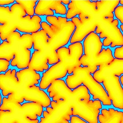
Materials 2021, 14, 3393                                                                                            3 of 22

                           the diffusion equation may lead to obtaining excessive values of the alloy component
                           concentration in the interface cell with an increase in the solid fraction. This problem
                           was found by several researchers [15,17,18,27]. To reduce overproduction of a component,
                           interface cells are treated as liquid phase cells when solving the mass transport equation.
                           Moreover, in most diffusion-controlled CA models [15,17,18,24–26], the growth rate is
                           calculated assuming a local equilibrium on the liquid-solid interface. This assumption
                           can only be considered valid in the case of steady-state growth. In the initial period of
                           unstable growth, the amount of the rejected component is too high to be transported from
                           the solidification front by a diffusion mechanism. Therefore, the acceptance of the mass
                           balance condition at the solidification front cannot be satisfactory for this period [18].
                                The article presents a 2D model for the numerical simulation of dendritic solidification
                           of a two-component alloy on the example of Al + 5 wt.% Mg. While building the CA
                           model, particular attention was paid to the problem of calculating the alloy component
                           concentration in the interface cells. The growth rule was based on the mass balance of the
                           component to calculate the appropriate component concentrations at the solidification front
                           and in the liquid and solid phases. At the same time, limitations on the maximum speed of
                           solid phase growth in the time interval were introduced. For the adopted growth rule, the
                           diffusion equation was solved in two stages with a pseudo-initial condition. The developed
                           methodology made it possible to determine the instantaneous component concentrations
                           at the solidification front, taking concentration and capillary undercooling into account.
                           For the initial period of unstable growth, the procedure of discarding component to the
                           nearest neighbouring cells was applied. The multi-grid method was also used in the paper
                           to solve the heat transport equation in order to shorten the calculation time. The developed
                           model allows for a realistic reconstruction of the dendrite morphology during solidification
                           of the binary alloy and is consistent with the results of the Derivative Differential Thermal
                           Analysis (DDTA) experiment and analyses of the chemical composition of EDS.

                           2. Description of the Model
                                Modelling of the dendritic structure evolution was performed using the cellular au-
                           tomaton technique in combination with the control volume method. The calculations were
                           performed on a flat area divided by a regular square grid into elementary cells with side
                           a. The following basic quantities were defined on the automaton grid: temperature—T,
                           concentration of the ingredient—W, solid phase fraction—f S , preferential angle of crystal-
                           lographic orientation—θ0 , interface curvature—K, direction normal to the solidification
                           front—ϕ. During solidification, each cell changed its phase state from liquid (f S = 0) to
                           transitional (0 < f S < 1) and finally to solid state (f S = 1). Initially, the temperature and
                           concentration distribution across the domain was homogeneous and consistent with the
                           values T0 and C0 . The model uses the von Neumann neighbourhood to solve the mass
                           and energy transport equations, and the Moor neighbourhood to determine the remaining
                           quantities. In order to reduce the artificial anisotropy of dendritic growth induced by the
                           CA grid, the procedure of following the preferred growth directions was applied [30]. The
                           quantitative and qualitative description of the growth kinetics of dendritic crystals is repre-
                           sented by three basic fields: solid fraction field, concentration field and temperature field.
                           The instantaneous interface location and the instantaneous shape of dendritic structures
                           are recreated by conjugate solving of the system of model equations.
                                The concept of the model assumes that the dendrite growth rate is controlled by
                           the component discharge rate from the solidification front by the diffusion mechanism.
                           The growth driving force is determined by the deviation from the equilibrium state, and
                           its measure is determined by the difference between the instantaneous local equilibrium
                           concentration and the instantaneous local chemical composition of the liquid phase. The
                           equilibrium concentration results from the thermodynamic relationship between the liq-
                           uidus temperature and the front curvature. The instantaneous temperature field and the
                           front shape determine the temporary distribution of the equilibrium concentration in the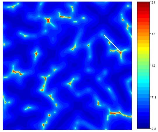
Materials 2021, 14, 3393 4 of 22
interface cells, while the concentration gradient formed in the front determines the growth
rate of the solid phase.
2.1. Modelling of Component Diffusion and Solid Phase Growth
The 2D diffusion equation with the effective diffusion coefficient was used to describe
the component transport:
∂2 W ( x, y, t) ∂2 W ( x, y, t)
∂W ( x, y, t)
= De f + (1)
∂t ∂x2 ∂y2
Effective Diffusion Coefficient Def depends on the phase state of the central cell and
the configuration of the cells of the immediate surroundings at the moment t and takes
homo- and heterogeneous neighbourhoods into account:
0.5 ( DS + DL ) f or (0 < f S,i,j < 1) and (0 < f S,Ne < 1)
De f = k D f or ( f S,i,j > 0) and ( f S,Ne = 1) (2)
0 S
DL f or ( f S,i,j < 1) and ( f S,Ne = 0)
where: fS,i,j , fS,Ne are solid phase fractions in the central cells i,j and in neighbouring
cells (von Neumann neighbourhood), respectively, DS , DL are the diffusion coefficients
of the component in the liquid and solid phases, respectively, and k0 is the component
separation coefficient.
During the growth of dendritic structures, interphase boundaries can be concave, flat
and convex, and the surface tension demonstrates anisotropy in the privileged crystallo-
graphic directions (of crystal growth). As a result, there are local changes in the equilibrium
solidification temperature at the front at the same component concentration. The paper
uses the modified Gibbs-Thomson equation, which allows for determining the change
in the equilibrium temperature in the function of concentration undercooling and the
solidification front curvature:
T F = TL + m L (WLF − W0 ) − Γ{1 − δ cos [mS ( ϕ − θ0 )]}K (3)
where: θ 0 —preferential angle of crystallographic orientation, δ—surface tension amplitude,
ms —crystal symmetry coefficient (ms = 4), K—interface curvature, ϕ—direction normal to
the solidification front, mL —direction coefficient of the liquidus line, G—Gibbs-Thomson
coefficient, TF —solidification front temperature, TL —liquidus temperature, W 0 —the initial
component concentration.
By transforming Equation (3), the dependence that determines the equilibrium com-
ponent concentration on the interface is obtained:
1 F
WLF = W0 + T − TL + ΓK {1 − δ cos[mS ( ϕ − θ0 )]} (4)
mL
To calculate the instantaneous increments in the solid fraction in the interface cells, the
mass balance equation, which after differentiation with respect to time and approximation
by the differential quotient is expressed by the following formula, was used:
t ∆f t +1
S,i,j + k 0 (WL,i,j − WL,i,j ) f S,i,j − WL ∆ f S,i,j +
k0 WL,i,j t t t
t +1 t )(1 − f t ) = ∆W (5)
(WL,i,j − WL,i,j S,i,j i,j
Calculations are performed in two stages. In the first stage, mass transport is also
solved and the change in concentration ∆W is determined assuming that the increment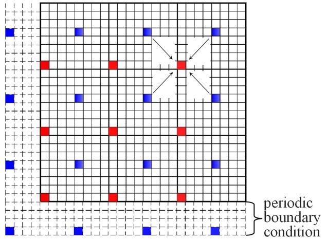
Materials 2021, 14, 3393                                                                                               5 of 22

                           of the solid fraction is zero (∆fS = 0, pseudo-initial condition). As a result, the component
                           concentration in the cells of the interface decreases to the value:

                                                         t+1,pseudo      t
                                                                                           ∆Wi,j
                                                      WL,i,j          = WL,i,j +          t ( k − 1)
                                                                                                                          (6)
                                                                                    1 + f S,i,j 0

                                                                                                                 t+1,pseudo
                                In the second stage, it is checked which cells of the concentration interface WL,i,j
                                                                        F . For cells in which the condition is met
                           are less than the equilibrium concentration WL,i,j
                             t+1,pseudo     F the value of the equilibrium concentration is entered W t+1 = W F and
                           WL,i,j     < WL,i,j                                                         L,i,j  L,i,j
                           it determines the increment of the solid phase on the basis of the transformed Formula (5):

                                                             ∆Wi,j − (WL,i,j
                                                                       F − W t )[1 + f t ( k − 1)]
                                                                             L,i,j    S,i,j 0
                                               ∆ f S,i,j =                  t ( k − 1)
                                                                                                                          (7)
                                                                           WL,i,j 0

                                In the remaining cells of the interface, the concentration values are determined from
                                                           t +1     t+1,pseudo
                           the pseudo-initial condition WL,i,j  = WL,i,j       . The chemical composition of liquid and
                           solid cells is also determined using Equation (6) substituting, accordingly, fS = 0 and fS = 1.
                                Based on the calculated increments of the solid fraction for each step ∆t f the normal
                           growth rate υn is determined from dependence [15,18,19]:

                                                                                    ∆x
                                                                       υn = ∆ f s                                         (8)
                                                                                    ∆t f
                                In the adopted procedure, a temporary “stop” of the solidification front allows for
                           determining the instantaneous component discharge rate from the interface cells and its
                           concentration in the liquid phase. Then, by comparing the value of this concentration
                           with the value of the equilibrium concentration, it is possible to determine the cells that
                           are involved in the transformation and their deviation from the equilibrium state. The
                           size of the increments of the solid phase is essentially influenced by the concentration
                           gradient on the side of the liquid phase, as well as the shape of the front curvature and
                           the temperature field, whereby the last two variables are used to determine the local
                           equilibrium concentration. Moreover, the proposed method of calculating the increments
                           of the solid fraction takes into account the change in the component concentration in
                           the solid and liquid phases during the passage of the solidification front through the
                           interface cell.
                                Solving Equation (4) requires determining the direction normal to the solidification
                           front in the interface cell. Three methods of determining this value are most often used
                           in CA models. The first one uses the procedure of tracking the position and topology of
                           the interface [31,32], the second one is based on the determination of the centre of mass of
                           the block of cells in the closest surrounding [27,30], and in the third one, calculations are
                           performed on the basis of solid fraction gradients. In order to ensure quick calculations
                           while maintaining high accuracy of the results, the last of the following variants was
                           applied to the model:                      "
                                                                                 ∂ f S −1
                                                                                     #
                                                                         ∂ fS
                                                           ϕ = arctan                                                (9)
                                                                         ∂x      ∂y

                               The last variable in Equation (4) is the interface curvature. Also, in this case, several
                           methods of determining the shape of the solidification front can be used [15,18,19,33]. The
                           quickest, but the least precise, are the procedures for counting the solids fraction on cell
                           blocks 3 × 3 or 5 × 5. The methods that use solid fraction gradients are more accurate.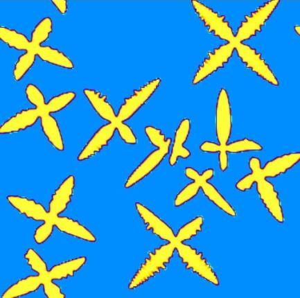
Materials 2021, 14, 3393                                                                                                          6 of 22

                           The modelling uses the dependence that was first proposed by Kothe [34]: the interface
                           curvature is determined on the basis of first and second order partial derivatives:
                                  "                             2                         2          # "                 # − 32
                                 ∂ f ∂ f ∂2 f S                      ∂2 f S                     ∂2 f S      ∂ fS 2     ∂ fS 2

                                                         ∂ fS                       ∂ fS
                             K= 2 S S           −                           −                           ×          +                (10)
                                 ∂x ∂y ∂x∂y              ∂x          ∂y2            ∂y          ∂x2         ∂x         ∂y

                           2.2. Temperature Field Approximation and Interpolation
                                 Solving a thermal problem on a cellular automaton grid with the use of explicit
                           diagrams is numerically ineffective. The stability of these methods [18,26] requires limiting
                           the time step to approximately 10−9 s in the case of modelling the Al alloys solidification
                           on a CA grid with a dimension of 1 µm. In order to overcome this inconvenience, implicit
                           methods are used, or a temperature that varies in time, but is homogeneous, is assumed for
                           the entire calculating area [4,12–14]. Another variant that was adapted to the model is the
                           determination of the temperature field using two grids. A sparse grid was superimposed
                           on the main CA grid, the constant of which (∆xB ) is several times larger than the automaton
                           cell dimension a. A block of cells with dimension nB × nB on the main grid corresponds to
                           a single cell of the sparse grid. Feedback occurs between the grids. On the sparse grid, for
                           each time interval, the heat transport equation is solved, and the determined temperature
                           field is interpolated into the main grid of the automaton. In turn, the instantaneous
                           increments of the solid fraction calculated in CA unit cells are summed up on blocks and
                           transferred to the sparse grid.
                                 The temperature field in the domain discretized by the sparse grid was calculated on
                           the basis of the equation:
                                                                 2
                                                                 ∂ T ( x, y, t) ∂2 T ( x, y, t)

                                             ∂T ( x, y, t)                                          L ∂ f SB
                                                           = aB                +                  +                                 (11)
                                                  ∂t                 ∂x2             ∂y2            c ∂t

                           where: c—specific heat, L—heat of solidification, a B —average thermal diffusivity.
                                The increments of the solid fraction in the sparse grid cells were calculated from
                           the dependence:
                                                                         ∑ ∆ fS
                                                              ∆ f SB =                                         (12)
                                                                        nB × nB
                                 The interpolation of the temperature field onto the main grid of the automaton was
                           carried out based on the procedure of a systematic transition from the distant to the nearest
                           neighbourhood (Figure 1). The calculations start with solving the heat transport equation
                           and determining the temperature field on the sparse grid (Figure 1a). Then the obtained
                           temperatures are transferred to the central cells of the CA main grid (Figure 1b). The
                           blocks on the main grid were placed in such a way so that the dimension of a single block
                           nB × nB met the relation 2n × 2n elementary cells (n—natural number). The temperature
                           interpolation from the central cells to the entire √
                                                                              main grid is√carried out in 2n steps. In the
                           first step, the temperatures in the cells (±2n−1 a 2, ±2n−1 a 2 ) located from central cells
                           are calculated. The obtained values together with the rewritten ones constitute the input
                           data for the second step, in which the temperatures in the cells from the environment are
                           determined (±2n−1 a, ±2n−1 a). In the third
                                                                     √ and fourth
                                                                                √ steps, interpolation is performed
                           based on the neighbourhoods (±2n−2 a 2, ±2n−2 a 2 ) and (±2n−2 a, ±2n−2 a). The proce-
                           dure is continued by systematically reducing the distance between cells in the main and
                           intermediate directions by half (according to the wind rose). Moving from the distant to
                           the nearest neighbourhood, the temperatures in all cells of the automaton are determined.
                           Since the distance between the cells is the same in each step, the interpolation problem
                           comes down to calculating the mean of the four surrounding cells. The interpolation
                           scheme on a fragment of the main grid with blocks with a dimension of 23 × 23 for the
                           next two steps is illustrated in Figure 1c,d. The diagram shows the solution using the
                           periodic boundary condition at the ends of the cellular automaton. The sparse grid size is
                           determined by the ratio ∆xB = 2n a.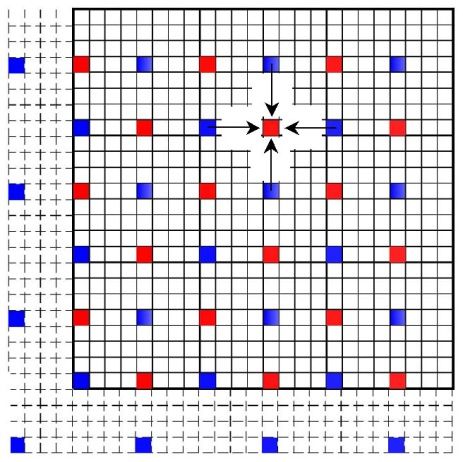
problem comes down to calculating the mean of the four surrounding cells. The inter-
polation scheme on a fragment of the main grid with blocks with a dimension of 23 × 23
for the next two steps is illustrated in Figure 1c,d. The diagram shows the solution using
Materials 2021, 14, 3393 7 of 22
the periodic boundary condition at the ends of the cellular automaton. The sparse grid
size is determined by the ratio ΔxB = 2na.
(a) (b)
(c) (d)
Figure 1. Diagram of temperature interpolation on a fragment of the main grid with blocks of size 23 × 23 for two
Figure 1. Diagram
consecutive stepsofoftemperature
calculations. (a) interpolation ontemperature
calculation of a fragmentfield
of the
on main
coarsegrid with
lattice; (b)blocks ofofsize
Transfer 23 × 23 for two
temperatures fromcon-
secutive steps
a coarse of calculations.
lattice to central cells (a)ofcalculation of temperature
CA blocks; (c) fieldofonaverage
step 1. calculation coarsetemperature
lattice; (b) Transfer of temperatures
on the basis of neighborhood from a
n − 1
√ n − 1
√ n − 1 n − 1
coarse lattice to central cells of CA blocks; (c) step 1. calculation of average temperature on the basis of neighborhood
(± 2 a 2, ± 2 a 2 ) ; (d) step 2. calculation of average temperature on the basis of neighborhood (± 2 a, ± 2 a ) .
(±2 n −1 a 2 ,±2n −1 a 2 ) ; (d) step 2. calculation of average temperature on the basis of neighborhood ( ±2 n−1 a,±2 n−1 a )
2.3. Nucleation and Initial Growth Period under Transient Diffusion Conditions
The cellular
2.3. Nucleation andautomaton technique
Initial Growth Period allows for modelling
under Transient of the
Diffusion nucleation stage using
Conditions
deterministic or probabilistic relationships. The models use the variants of immediate
The cellularnucleation.
and continuous automatonThe technique allows for modelling
initial distribution of the
of cells called nucleation
nuclei in the stage using
calculating
deterministic
domain or probabilistic
is usually determinedrelationships.
at random, after The models
reachinguse thethe variants of
appropriate immediate
temperature
and continuous nucleation. The initial distribution of cells called nuclei
(depending on the adopted nucleation model). Neighbouring cells are joined to nucleus cells in the calculating
domain
to form an is interface
usually determined
that evolves at random,
based after reaching
on accepted the appropriate
growth rules. In the presentedtemperature
model,
(depending on the adopted nucleation model). Neighbouring
it was assumed that nucleation occurs immediately, and that the solidification cells are joined toprocess
nucleus
cells to after
begins form reaching
an interface that evolvestemperature
the nucleation based on accepted
TN which growth
is lessrules.
than TIn the presented
L . Temperature
model,
T it was assumed that nucleation occurs immediately, and that the solidification
N depends directly on the rate of cooling and diffusion of the component in the liquid
processThe
phase. begins
ideaafter
of thereaching
algorithm theisnucleation
as follows.temperature TN which
Once the liquidus is less than
temperature is TL. Tem-
reached,
perature T depends directly on the rate of cooling and diffusion of
a randomised location of nucleus cells is determined in the CA area, and it is assumed
N the component in the
liquid phase. The idea of the algorithm is as follows. Once the liquidus
that the proportion of the solid phase in them is one. The formation of nucleus cells is temperature is
related to the “production” of an excess of the alloy component ∆W = WL − WS . It is
reached, a randomised location of nucleus cells is determined in the CA area, and it is
assumed that the proportion
componentof is the solidrejected
evenly phase in to them is one.
all cells in theThe formation
Moore of and
vicinity nucleus
its
concentration in each of these cells is increased by the amount ∆W/8. From that moment
on, the procedure for solving the diffusion equation is started. The initial increase in the
component concentration around nucleus cells makes them inactive for a certain period of
time. Only as a result of channelling the component deep into the bath and dissipating
superheat, they are able to connect their neighbours. This occurs as soon as neighbouring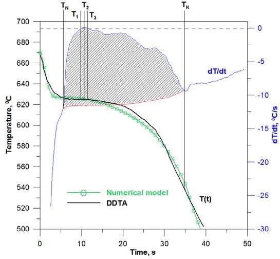
Materials 2021, 14, 3393                                                                                           8 of 22

                           cells reach temperature TF , determined by Equation (3). Temperature TF is considered the
                           nucleation temperature TN, and the time needed for lowering the temperature from TL to
                           TN an incubation period.

                           2.4. Optimisation of the Time Step for Model Equations
                                The use of the iterative process for explicit numerical schemes described in the pre-
                           vious chapters is related to the determination of the limit value of time step ∆tstab which
                           ensures the stability of the calculations. The stability condition for the numerical solution
                           of the diffusion equation is expressed by the dependence:

                                                                   DL ∆tW
                                                                          < 0.25                                    (13)
                                                                    ∆x2
                           while the energy equations on the sparse grid ∆xB :

                                                                   a B ∆t T
                                                                            < 0.25                                  (14)
                                                                    ∆x2B

                                 Apart from these two components, step ∆tstab is also limited by an additional criterion
                           that relates to the speed at which the solidification front moves through the interface cell.
                           In order to ensure high “precision” of calculations, the increment of the solid fraction in
                           one step of the calculations must be sufficiently small. The construction of the automaton
                           assumes that the cell changes its state from transient to solidified at the moment when the
                           solid fraction reaches one, and exceeding this value is omitted. Moreover, due to the use
                           of an explicit scheme to solve the diffusion equation, excessive solid phase growth can
                           lead to overestimated values of the component concentration in the interface cells. It was
                           established in [27] that the elementary increment of the solid phase ∆f el in one-time step
                           should be in the range (0.01–0.1). Following these guidelines and preliminary simulations,
                           it was assumed that the maximum increment in one step of the calculations was 0.02. By
                           inserting this value into Equation (8) and taking dependencies (13) and (14) into account,
                           the time step limitation is obtained in the form of the formula:
                                                                                                  !
                                                                      ∆x2         ∆x         ∆x2B
                                                   ∆tstab = min 0.25       , 0.02 max , 0.25                        (15)
                                                                       DL        υn           aB

                                Above the liquidus temperature, only the thermal problem for which ∆tstab = ∆tT is
                           solved. After the liquidus temperature is exceeded, optimization of the time step is done
                           with regard to quantity ∆tf , comparing it with ∆tT and ∆tW . For high solids growth rates,
                           upper limit ∆tstab is related to the second term of formula (15), while for medium and low
                           velocities, it is related to the stability of the explicit scheme of the thermal conductivity
                           equation. Due to step ∆tT , despite the use of the multi-grid technique, it can be several
                           dozen times smaller than steps ∆tf or ∆tW ; in order to shorten the calculating time, the
                           algorithm uses a separate iteration procedure for the thermal problem. In this procedure,
                           the number of iterations based on the ratio ∆tf /∆tT or ∆tW / ∆tT are determined. The
                           isolation of the energy equation means that the remaining model equations can be solved
                           with the limitation for ∆tf or ∆tW . Optimization is performed for each iteration, and a set
                           new value ∆tstab is valid for the next step. No calculations are updated for the current step.

                           3. Numerical Simulations Results
                           3.1. Free Growth of a Single Dendrite
                                Computer simulations of the free dendrite growth were carried out on the Al + 5 wt.%
                           Mg using the material parameters from references [27,33,35]. The calculations were per-
                           formed on a cellular automaton with elementary cells with dimension of 160 × 160, which
                           corresponds to a flat area of 320 × 320 µm2 . The side length of the cell was selected
                           empirically. If the value “a” of the cells is selected too high, the shape of the growing main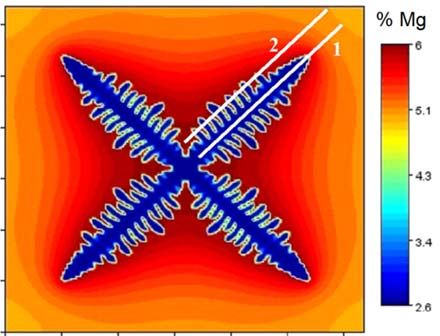
Materials 2021, 14, 3393                                                                                                         9 of 22

                                       arms of the dendrite ceases to depend on their preferential crystallographic orientation
                                       and begins to depend only on the symmetry of the CA grid. For the cooling rates used in
                                       the simulations, the growth of dendrites in the direction corresponding to their assumed
                                       orientation is obtained for a cell side length of up to 2 µm. The diffusion equation was
                                       solved assuming a periodic boundary condition at all ends of the CA grid. For the energy
                                       equation, it was assumed that the heat dissipation from the modelled area occurs perpen-
                                       dicular to its surface and at a constant value of the heat flux—the boundary condition of the
                                       second type. After exceeding the temperature TL one nucleus cell was placed in the centre
                                       of the calculating domain. This cell was assigned an orientation angle that is inconsistent
                                       with both of the major directions of the CA grid. Preferential angle of crystallographic
                                       orientation θ0 was 25◦ .
                                             The next Figure 2a–c present the results of the simulation of the influence of the cooling
                                       rate on the development of dendritic structures and the accompanying instantaneous fields
                                       of the component concentration in the liquid, solid and transition phases. The interface
                                       cells show the average Mg concentration values resulting from the mass balance. The
                                       calculations were made for three cooling rates, the values of which, in the absence of an
                                       internal heat source, are: 5 K/s, 25 K/s and 45 K/s.

                            (a)                                  (b)                                (c)

      Figure  2. Instantaneous Mg concentration fields and free dendrite growth sequences in the Al + 5 wt.% Mg alloy cooled at
         Figure 2. Instantaneous Mg concentration fields and free dendrite growth sequences in the Al + 5% wt. Mg alloy
      the rate: (a) 5 K/s, (b) 25 K/s, (c) 45 K/s.
         cooled at the rate: a) 5 K/s, b) 25 K/s, c) 45 K/s.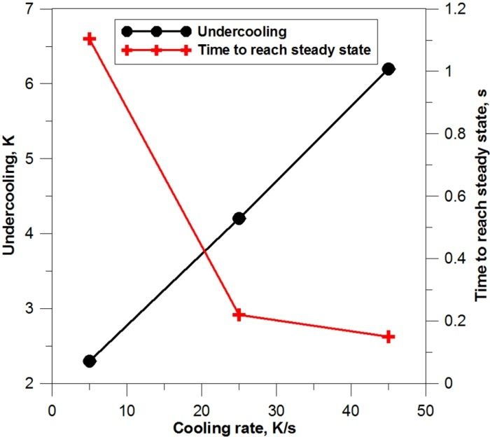
Materials 2021, 14, 3393                                                                                            10 of 22

                                  On the basis of the obtained simulation results, the sequences of free growth of the
                           dendritic crystal can be traced. In its initial stage, the solid phase grows on a square nucleus
                           cell, changing the original shape to a circle. This circular form, characteristic of the onset of
                           dendritic solidification, is further disturbed fourfold in mutually perpendicular directions.
                           As a result, the isotropic structure is transformed into a square whose vertices are oriented
                           by the preferential angle. After some time, the growth of the vertices of the square leads
                           to the formation of four first-order branches. For a low cooling rate (5 K/s), only main
                           dendrite branches are formed, while for medium and high cooling rates, characteristic
                           disturbances of the surface of the first-order branches appear, from which the secondary
                           branches crystallize.
                                  As the cooling rate increases, the distance between the axes of the side branches and
                           the transverse dimension of the main branches decrease. At medium and high cooling
                           rates, the first order branches increase their transverse dimensions only in the vicinity of
                           the dendrite front. Secondary branches grow below this zone and inhibit further transverse
                           growth of the main branch. As a result, the main branches have a uniform cross-section
                           along their entire length. Such a property does not occur for the cooling rate of 5 K/s and
                           the largest transverse dimension of the main branch appears above half its length, counting
                           from the base of the dendrite. At the highest cooling rate (45 K/s), the growth rate of the
                           side branches’ front clearly increases. As a result, the difference between the length of the
                           main branches and the length of the side branches decreases.
                                  In models using the CA technique, the equations of thermal conductivity and diffusion
                           are solved in a conjugate manner, which makes it possible to track the change in component
                           concentration in the growing dendrite, at the solidification front and the surrounding
                           liquid phase. On a local scale, a change in the state of the system, which is related
                           to the segregation of the component in the liquid and solid phase, is observed. The
                           degree of component segregation depends mainly on the shape of the formed structures,
                           their characteristic dimensions, the size of the solidification temperature interval, and
                           the diffusion and cooling rate. In the initial solidification period, first of all, the uneven
                           distribution of the alloy component in the liquid phase is observed, while in the solid
                           phase, segregation is negligible due to the very small dimensions of the dendrite and
                           short diffusion paths. Based on Figure 2, it can be concluded that with the free growth of
                           dendrites, the phenomenon of segregation in the liquid phase intensifies with the increase
                           in cooling rate. At a cooling rate of 45 K/s, the liquid phase enriched with the alloy
                           component occupies only a small area around the dendrite arms: the diffusion layer
                           is practically in the immediate vicinity of the solid phase. In the remaining liquid, the
                           component concentration is equal to the initial concentration C0 .
                                  Figure 3b shows the instantaneous alloy component concentration fields in the suc-
                           cessive phases of dendrite growth at a cooling rate of 45 K/s. The profiles were marked
                           along the line being the symmetry axis of the main branch of the dendrite (Figure 3a). From
                           the graph presented in Figure 3b, the instantaneous width of the diffusion layer in front
                           of the dendrite as well as the instantaneous Mg concentrations in the tip interface cells
                           can be read. In the initial stage of solidification, the component concentration at the front
                           increases rapidly and reaches a maximum value of approx. 6.3% Mg. After this period,
                           the crystal begins to grow under the set diffusion conditions and the Mg concentration
                           remains practically at the same level. The highest concentration of the alloy component,
                           regardless of the cooling rate, occurs at the base of the dendrite, in interdendritic spaces
                           (for cooling rates of 25 K/s and 45 K/s) and in front of the main branches’ front. A typical
                           distribution of the alloy component along the section starting from the base of the dendrite
                           and crossing the secondary arms (line 2 in Figure 3a) is presented in graph 3c. The high
                           value of Mg concentration in the distinguished places inhibits the lateral growth of the
                           main branches and contributes to the development of secondary branches, the fronts of
                           which move towards the zone with a lower component concentration.
spaces (for cooling rates of 25 K/s and 45 K/s) and in front of the main branches’ front. A
typical distribution of the alloy component along the section starting from the base of the
dendrite and crossing the secondary arms (line 2 in Figure 3a) is presented in graph 3c
The high value of Mg concentration in the distinguished places inhibits the lateral growth
Materials 2021, 14, 3393 of the main branches and contributes to the development of secondary11branches,
of 22 the
fronts of which move towards the zone with a lower component concentration.
(a)
(b) (c)
Figure 3. The results
Figure of the
3. The simulation
results of the equiaxial
of the simulation of thedendrite
equiaxialgrowth forgrowth
dendrite the cooling rate
for the of 45 K/s:
cooling rate (a) theK/s:
of 45 morphology
(a) the morphology
of the dendrite ◦
of thewith orientation
dendrite θ 0 = 45 , (b)
with orientation θ0 Mg concentration
= 45°, profiles during
(b) Mg concentration dendrite
profiles duringgrowth
dendritedetermined along linealong
growth determined 1, line 1,
(c) magnesium distribution
(c) magnesium along the section
distribution starting
along the from
section the base
starting of the dendrite
from and
base of the crossingand
dendrite thecrossing
secondary thearms (line 2)arms (line
secondary
− f S = 0.1.2) − fS = 0.1.
LoweringLowering
the cooling
therate to 25 rate
cooling K/stocauses
25 K/sthe zone the
causes of the liquid
zone phase
of the liquidenriched with
phase enriched with
alloy component to increase
alloy component to and the maximum
increase Mg concentration
and the maximum values invalues
Mg concentration the interface
in the interface
cells to decrease. Lower cooling
cells to decrease. Lower rates
cooling correspond to lower to
rates correspond concentration gradientsgradients
lower concentration in in
front of the solidification front and, as a result, lower crystal growth rates and
front of the solidification front and, as a result, lower crystal growth rates and large larger
distancesdistances
between secondary branches. For
between secondary a low cooling
branches. For a lowratecooling
(5 K/s),rate
the alloy component
(5 K/s), the alloy compo
segregation phenomenon is not so intensely visible. The area of the enriched
nent segregation phenomenon is not so intensely visible. The area of the enriched liquid phase liquid
becomes phase
more blurred, and the Mg concentration in the transition cells at the beginning
becomes more blurred, and the Mg concentration in the transition cells at the be
of solidification does not exceed 5.4%. Figure 4a shows the change in the component
concentration at the solidification front depending on the solid phase share (dendrite
size) and the cooling rate. The obtained curves illustrate the two essential periods of
dendrite growth at the beginning of solidification. The first period, which is characterised
by transient conditions of component diffusion in the liquid and occurs with increasing
concentration of magnesium at the solidification front, and the second period of growth,
which occurs at a relatively equal component concentration at the front and approximately
corresponds to the established diffusion conditions. After the liquidus temperature isponent concentration at the solidification front depending on the solid phase share
(dendrite size) and the cooling rate. The obtained curves illustrate the two essential pe-
riods of dendrite growth at the beginning of solidification. The first period, which is
characterised by transient conditions of component diffusion in the liquid and occurs
Materials 2021, 14, 3393 with increasing concentration of magnesium at the solidification front, and the second 12 of 22
period of growth, which occurs at a relatively equal component concentration at the front
and approximately corresponds to the established diffusion conditions. After the liqui-
dus temperature is exceeded, according to the nucleation procedure described in Section
exceeded, according
2.3, one nucleus cell isto the nucleation
placed procedure
in the middle of the described
automatoninand
Section 2.3, one
the excess nucleus cell
component is
is placed in the middle of the automaton and the excess component is rejected
rejected to cells in Moore’s neighbourhood. These cells become active at temperature to cells TinN
Moore’s neighbourhood. These cells become active at temperature TN where the growth of
where the growth of the dendrite begins. However, due to the very small number of in-
the dendrite begins. However, due to the very small number of interface cells, the amount
terface cells, the amount of generated solidification heat is still very small and the tem-
of generated solidification heat is still very small and the temperature is further lowered.
perature is further lowered. At the same time, the degree of concentration undercooling
At the same time, the degree of concentration undercooling and the growth rate of the solid
and the growth rate of the solid fraction increase. Over time, the dendrite surface (inter-
fraction increase. Over time, the dendrite surface (interface) becomes larger and the growth
face) becomes larger and the growth rate is intensified, resulting in the release of more
rate is intensified, resulting in the release of more solidification heat and the suppression
solidification heat and the suppression of the temperature drop. The local minimum for
of the temperature drop. The local minimum for which the solidification heat is equal to
which the solidification heat is equal to the cooling rate is revealed in the solidification
the cooling rate is revealed in the solidification curve. The minimum temperature also
curve. The minimum temperature also corresponds to the maximum degree of under-
corresponds to the maximum degree of undercooling of the alloy and the maximum growth
cooling of the alloy and the maximum growth rate of the solid fraction.
rate of the solid fraction.
(a) (b)
Figure 4. (a)
Figure 4. (a)changes
changesininthe
theconcentration of of
concentration magnesium
magnesium at the solidification
at the frontfront
solidification depending on the
depending onshare of the of
the share solid
thephase
solid
(dendrite size) and
phase (dendrite different
size) cooling cooling
and different rates, (b)rates,
changes in the average
(b) changes in the temperature in the initial
average temperature period
in the of crystal
initial period growth.
of crystal
growth.
The further expanding dendrite interface combined with the high growth rate causes
the rate
Theoffurther
solidification heat generated
expanding dendrite to exceed the
interface cooling rate,
combined with andthe the metal
high is heated.
growth rate
The effect
causes theof theoftemperature
rate solidification increase is, in turn,
heat generated to aexceed
slight the
decrease
coolingin rate,
Mg concentration
and the metalat is
the solidification
heated. The effectfront
of the(Figures 3a andincrease
temperature 4a) andis, theingrowth rate, which
turn, a slight decreasecauses theconcen-
in Mg rate of
heating the
tration at metal
the to gradually
solidification frontdecrease.
(FiguresThe 3a system
and 4a)re-establishes
and the growth a state
rate,where
whichthe rate
causes
of solidification heat is equal to the rate of cooling and a local maximum
the rate of heating the metal to gradually decrease. The system re-establishes a state appears in the
solidification curve. The temperature recalescence effect is particularly
where the rate of solidification heat is equal to the rate of cooling and a local maximum pronounced at a
cooling rate of 45 K/s. With the increase of the cooling rate, the maximum
appears in the solidification curve. The temperature recalescence effect is particularly undercooling of
the alloy and at
pronounced thea temperature
cooling raterangeof 45 of recalescence
K/s. increase, of
With the increase and thecooling
the local minima move
rate, the maxi-to
higher shares of the solid
mum undercooling of thefraction
alloy and(Figure 4b).
the temperature range of recalescence increase, and
the local minima move to higher shares of the solid fraction (Figure 4b).
3.2. Validation of the Numerical Model
In order to determine the potential of the numerical model, the results of the CA
simulation were compared with the LGK analytical model. The validation was performed
using the guidelines proposed by Zhu and Stefanescu in paper [18]. Figure 5a shows
the evolution of the dendrite front growth rate in the model area cooled at the rate of
25 K/s. The values of the growth rate were determined in the interface cells in which
the solid fraction was within the range of 0.2–0.8. The presented kinetic pattern indicates
that the dendrite growth under transient diffusion conditions takes about 0.2 s. After this
time, the growth rate becomes constant and at the same time the highest value, and theIn order to determine the potential of the numerical model, the results of the CA
simulation were compared with the LGK analytical model. The validation was per-
formed using the guidelines proposed by Zhu and Stefanescu in paper [18]. Figure 5a
shows the evolution of the dendrite front growth rate in the model area cooled at the rate
of 25 K/s. The values of the growth rate were determined in the interface cells in which
Materials 2021, 14, 3393 13 of 22
the solid fraction was within the range of 0.2–0.8. The presented kinetic pattern indicates
that the dendrite growth under transient diffusion conditions takes about 0.2 s. After this
time, the growth rate becomes constant and at the same time the highest value, and the
further development of
further development ofthe
thedendrite
dendriteoccurs
occursapproximately
approximately under
under thethe established
established diffu-
diffusion
sion conditions. The obtained shape of the growth velocity curve is
conditions. The obtained shape of the growth velocity curve is different from the curvesdifferent from the
curves determined
determined in other in CA
other CA solidification
solidification models models [15,18,19]
[15,18,19] and results
and results fromfrom the ap-
the applied
plied nucleation
nucleation procedure.
procedure. In theIndeveloped
the developedmodel,model,
the the growth
growth raterate increases
increases fromfromzerozeroto
to
thethe maximum
maximum value,
value, which
which is physically
is physically consistent
consistent with
with thethe characteristics
characteristics of of
thethe ini-
initial
tial solidification
solidification period.
period. TheThe achievement
achievement ofofthethesteady
steadystate
statedepends
dependson onthe
the rate
rate of
of heat
dissipation from the model area (Figure (Figure 5).
5). For
For the
the cooling
cooling rate
rate of
of 55 K/s,
K/s, the time needed
to stabilize
stabilize the
the dendrite
dendrite front
front growth
growth rate
rate is
is the
the longest
longest and
and amounts
amounts to to more
more than
than 11 s.s.
Figure 5 also
also presents
presents thetheeffect
effectofofcooling
coolingrate
rateononthethevalue
valueofof concentration
concentration undercool-
undercooling
ing for the
for the steady
steady state.
state.
(a) (b)
Figure 5. Kinetic characteristics of the initial solidification period: (a) the growth rate of the dendrite front, (b) the effect of
cooling rate
the cooling rateon
onthe
theconcentration
concentrationundercooling
undercooling value
value andand
thethe transition
transition timetime
fromfrom the transient
the transient state state
to thetosteady
the steady
state.
state.
The comparison of the predictive parameters of the LGK model and the developed
CA model is presented
The comparison in Figure
of the 6a–c.parameters
predictive The tests of were
thecarried out by
LGK model anddetermining
the developed the
shape
CA of the
model is dendrite
presentedfront along with
in Figure 6a–c. itsTheapproximation by theout
tests were carried parabolic function the
by determining for
each undercooling value. The applied parabolic approximation ensures
shape of the dendrite front along with its approximation by the parabolic function for a high degree of
matching to the values calculated from the model. The determination coefficient R 2 reaches
each undercooling value. The applied parabolic approximation ensures a high degree of
a value above
matching 0.99.values
to the Figurecalculated
6a shows the calculation
from the model.results
Thefordetermination
a dendrite withcoefficient
the preferredR2
crystallographic orientation ◦
0 , growing with
reaches a value above 0.99. Figure 6a shows theundercooling 4.2 K. for
calculation results Based on the obtained
a dendrite with the
approximating
preferred functions, the
crystallographic curvature
orientation 0°,and then the
growing withdiameter of the dendrite
undercooling fronton
4.2 K. Based were
the
determined using dependence K = d 2 y/dx2 × [1 + (dy/dx)2 ]−3/2 and the relation R = 1/K.
obtained approximating functions, the curvature and then the diameter of the dendrite
The comparative
front were determinedcharacteristics of the dendrite
using dependence K = dtip diameter
2y/dx calculated
2 × [1 + (dy/dx) 2]−3/2from
and the
the numerical
relation R
model and the LGK analytical model for different undercooling
= 1/K. The comparative characteristics of the dendrite tip diameter calculated are shown in Figure 5b.
from the
The LGK model prediction was performed assuming stability parameter σ = 1/4π 2 . When
numerical model and the LGK analytical model for different undercooling are shown in
evaluating
Figure the test
5b. The LGK results,
modelit prediction
can be observed that both the
was performed obtainedstability
assuming parameter value range
parameter σ=
R as well as the tendency of its changes depending on undercooling are satisfactory. The
second real parameter that allows for validating the numerical model is the dendrite front
growth rate under the set diffusion conditions. Simulated growth rate (Figure 6c) also
presents a good agreement with the results predicted by the LGK model. However, it
should be noted that the values calculated from the numerical model are always below
the LGK curves. This fact was found in other papers [18,19,36] and is explained by the
sensitivity of the LGK model to parameter σ, which changes depending on undercooling
and the initial alloy composition.satisfactory. The second real parameter that allows for validating the numerical model is
the dendrite front growth rate under the set diffusion conditions. Simulated growth rate
(Figure 6c) also presents a good agreement with the results predicted by the LGK model.
However, it should be noted that the values calculated from the numerical model are
Materials 2021, 14, 3393
always below the LGK curves. This fact was found in other papers [18,19,36] and14 isofex-
22
plained by the sensitivity of the LGK model to parameter σ, which changes depending on
undercooling and the initial alloy composition.
Y = 0.00466 - 44.56 X X + 111422 X X2
0.000212
0.000208
y, m
0.000204
0.0002
0.00019 0.000195 0.0002 0.000205 0.00021
x, m
(a)
16 1
LGK model
LGK model
m/s
Present model
Steady state dendrite tip radius, 10 -6 m
Present model
-3
Steady state dendrite tip velocity, 10
12
8 0.1
4
0 0.01
2 4 6 8 2 4 6 8
Undercooling, K Undercooling, K
(b) (c)
Figure 6.
Figure 6. Comparison
Comparison of of the
the predictive parameters of
predictive parameters of the
the LGK
LGK model
model and
and the
the developed CA model:
developed CA model: (a)
(a) the
the shape
shape of
of the
the
dendrite front and its its parabolic
parabolic approximation,
approximation,(b)
(b)the
theeffect
effectofofconcentration
concentrationundercooling
undercoolingononthe
thedendrite
dendritefront diameter,
front diame-
ter, (c) effect
(c) the the effect of concentration
of concentration undercooling
undercooling on velocity
on the the velocity of dendrite
of the the dendrite front.
front.
3.3. Multiple Dendrite Growth Simulation
Simulation of the growth of many dendrites was conducted in the area of 816 × 816 µm2
using a cellular automaton with elementary cells sized 408 × 408. The diffusion equation
was solved assuming the same boundary conditions as in the previous simulations. On
the other hand, for the heat conduction equation on the lower and upper walls, a periodic
condition was assumed, and on the right wall—thermal symmetry qb = 0, and on the left
wall—Newton’s boundary condition:
qb = α( T − T∞ ) (16)
where: α—the heat transfer coefficient, T∞ —the bulk temperature of the cooling media.
The values of the heat transfer coefficient were selected so as to correspond to the
DDTA test conditions presented in the next chapter. Calculations were started assuming the
initial temperature T0 equal to 670 ◦ C. After reaching the liquidus temperature, 12 nucleus
cells with the initial composition kC0 and the preferred crystallographic orientation ranging
from 0◦ up to 90◦ were placed randomly in the calculating domain. Coupled motion and
interaction of equiaxial dendritic crystal growth during solidification of Al + 5 wt.% Mg
alloy is presented in Figure 7.Figure 5b. The LGK model prediction was performed assuming stability parameter σ =
1/4π2. When evaluating the test results, it can be observed that both the obtained
Materials 2021, 14, 3393 3.3. Multiple Dendrite Growth Simulation 15 of 22
media.
(a) (b) (c)
(d) (e) (f)
(g)
Figure 7. Multi-dendritic
Figure growth
7. Multi-dendritic sequence
growth in aninsolidifying
sequence Al +Al
an solidifying 5 wt.%. Mg Mg
+ 5 wt.% alloy: (a) 0.02,
alloy: (b) 0.1,
(a) 0.02, (c) 0.2,
(b) 0.1, (d) 0.45,
(c) 0.2, (e) 0.7,
(d) 0.45, (e) 0.7,
(f) 0.9 of solid fraction, (g) actual microstructure of the Al + 5 wt.%. Mg alloy cast into a metal mold (Section
(f) 0.9 of solid fraction, (g) actual microstructure of the Al + 5 wt.% Mg alloy cast into a metal mold (Section 4). 4).
In the initial
In the period
initial (Figure
period 7a–c)
(Figure main
7a–c) branches
main branches of dendrites
of dendrites with the the
with preferred
preferred
crystallographic
crystallographicorientation
orientation develop
develop from
fromnucleus
nucleuscells,
cells, and their growth
and their growthisisrelated
related pri-
primarily
marily
to the increase in longitudinal dimensions. At the same time, on the surface of thethe
to the increase in longitudinal dimensions. At the same time, on the surface of main
main arms,
arms, below
below thefront,
the front,seeds
seedsofofthe
thesecondary
secondaryarms
armsare are initiated.
initiated. The size
size and
andshape
shape of
the dendrites formed during this period depend on the initial distribution of nucleus cells,
preferential growth direction and coupled interaction between the crystals. The longest
main branches are characteristic of dendrites, the nuclei of which were located at a great
distance from others, and the free growth of the arms to the liquid regions lasted the
longest. Mutual close location of nucleus cells causes the interaction between the main arms
to occur in the initial stage of solidification, significantly reducing their size. Inhibition of
the longitudinal growth of the main branches causes their thickening and the developmentYou can also read