Capital Regulations and Credit Line Management during Crisis Times
←
→
Page content transcription
If your browser does not render page correctly, please read the page content below
Capital Regulations and Credit Line Management
                                            during Crisis Times∗

                                Paul Pelzla and Marı́a Teresa Valderramab

                       a
                           Tinbergen Institute (TI) & Vrije Universiteit Amsterdam (VU)
                                     b
                                         Oesterreichische Nationalbank (OeNB)

                                                November 4, 2018

                                                     Abstract
            Credit line drawdowns by firms reduce a bank’s regulatory capital ratio. Using the Austrian
        Credit Register we provide novel evidence that during the 2008-09 financial crisis, banks with
        a distressed capital position managed this concern by substantially cutting little-used credit
        lines. Controlling for a bank’s capital position, we also find that greater liquidity problems
        induced banks to considerably cut little-used credit lines over 2008-09. These results suggest
        that banks actively manage both capital and liquidity risk caused by undrawn credit lines in
        periods of financial distress, but thereby reduce liquidity provision to firms exactly when they
        need it most.

1       Introduction

Most European firms are bank-dependent, and a significant fraction of bank lending is done via
credit lines. A corporate credit line commits a bank to lend to a firm up to an agreed amount for
an agreed period of time, unless the firm violates a covenant. This makes credit lines a particularly
reliable source of debt financing (Sufi, 2009). From the granting bank’s perspective, commitment
fees charged on the unused portion of the line make up a considerable fraction of revenues from
    ∗
    We thank members of the Economic Analysis and Research Department of the Oesterreichische Nationalbank
(OeNB), the research department of De Nederlandsche Bank (DNB), Franklin Allen, Hans Degryse, Tim Eisert,
Aysil Emirmahmutoglu, Pirmin Fessler, Jakob de Haan, Franz Hahn, Steven Poelhekke, Doris Ritzberger-Grünwald,
Gunseli Tumer-Alkan and seminar participants at the OeNB, DNB, Tinbergen Institute, University of Amsterdam
and VU Amsterdam as well as conference participants at C.r.e.d.i.t. 2018 in Venice, the 6th WU-WAETRIX workshop
in Vienna, the 35th International Symposium of Money, Credit and Banking in Aix-en-Provence, the TI Jamboree
2018 in Amsterdam, the NOeG Annual Meeting 2018 in Vienna, the 5th Research Workshop of the MPC Task Force
on Banking Analysis for Monetary Policy in Brussels, the 1st NOeG Winter Workshop in Vienna and IFABS 2017 in
Oxford for helpful comments and suggestions.

                                                         1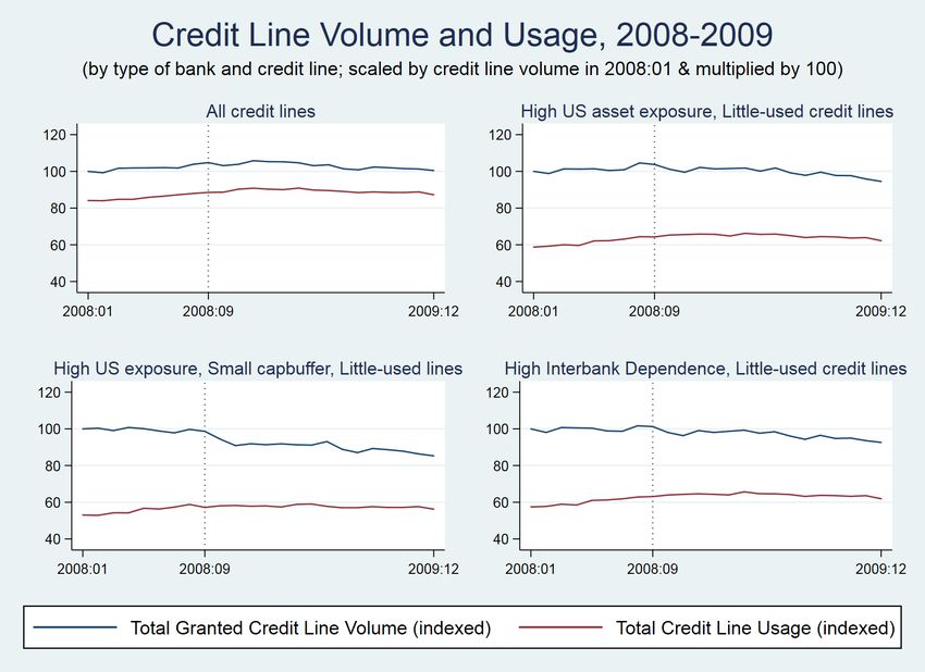
credit lines (Sufi, 2009; Loukoianova et al., 2006). These earnings come at relatively low cost for
the bank as long as the line remains unused. The reason is that from a regulatory perspective,
the undrawn portion of a credit line is largely off-balance sheet and must therefore be backed by
only little capital under the Basel framework. The flip-side is that additional drawdowns result
in a direct and possibly unexpected increase in a bank’s balance sheet and thus decrease in its
regulatory capital ratio. This reduces a bank’s buffer towards its minimum capital requirement,
which limits its potential to absorb future losses and also harms a bank’s stock market performance
(Demirguc-Kunt et al., 2013). Exposure to unused credit lines may therefore put a bank’s capital
buffer at risk. This source of risk has received virtually no attention in the academic literature, but
is far from negligible. Specifically, if the usage of all credit lines that we observe increased to match
their committed volume in early 2008, the average bank operating in Austria would have had to
increase its capital stock by up to six percent to keep its capital ratio and thus buffer constant.
Without raising extra capital, the bank would have suffered a decrease in its capital buffer by up to
15 percent. Since our data only covers the universe of relatively large credit lines, the total impact
may be considerably higher.

Sizable capital buffer reductions are particularly problematic in periods of financial distress. The
reason is that the capital position of banks is then typically weakened, raising capital is more costly
and credit line drawdowns are more likely. This raises the question whether and to what extent
banks actively manage capital concerns that come with exposure to undrawn credit lines in crisis
times, and what consequences this has on lending to the corporate sector. To the best of our knowl-
edge, we are the first to study this question. We find that during the 2008-09 financial crisis, banks
whose capital position was hit relatively hard and whose initial capital buffer was low reduced the
risk of capital ratio reductions by substantially cutting credit lines that were used relatively little
in relation to their granted volume at the onset of the crisis. These findings shed light on a novel
yet important link between bank capital regulations and lending to the real economy.
As a second contribution, we show that relatively large liquidity problems during the crisis also
induced banks to cut little-used credit lines over 2008-09 considerably and more than other banks,
controlling for a bank’s capital position. Thereby, banks with liquidity concerns limited the scope
of additional credit line drawdowns and the resulting costs. Our findings are conditional on changes
in firm-specific credit demand and bank-specific unobservables during the crisis. We therefore pro-
vide causal evidence that banks actively manage both capital and liquidity risk caused by exposure

                                                   2
to undrawn credit lines in periods of financial distress. From the perspective of banking system
stability, this is good news. However, the implication is that banks reduce liquidity provision to
firms exactly at a time in which they need it most and when alternatives to bank financing tend to
be scarce, especially in bank-dependent financial systems. This evidence is valuable since changes
in liquidity provision by banks to firms may have real consequences but have received limited at-
tention in the policy debate on the 2008-09 and other financial crises. The reason is that the debate
has mainly focused on variation in credit usage levels rather than commitment volumes.

Our primary data source is the Austrian credit register, which is ideally suited to pursue our re-
search goals. The register provides information on bank-firm specific credit commitments over time
and thus allows us to convincingly account for endogeneity issues such as heterogeneity in firm
credit demand and to control for bank unobservables. What’s more, the register provides infor-
mation on how much a firm makes use of a credit commitment in a given month, which allows
to measure the risk of additional drawdowns for each individual credit relationship we observe.
Data are available for the universe of banks and firms operating in Austria, as long as the credit
commitment or usage exceeds e350,000.
Not only due to the quality of data, but also from a conceptual perspective Austria is an ideal
setting to study our research questions. This is in part because Austrian banks have tradition-
ally had relatively low capital buffers compared to other countries (Fonseca and González, 2010).
Furthermore, for many Austrian banks it has been particularly difficult to raise external capi-
tal due to their ownership structure, as we explain in section 3. Austrian banks have therefore
been exceptionally sensitive to capital ratio reductions and thus additional credit line drawdowns.
Last, but not least, changes in bank credit commitment volumes are particularly crucial if banks
are by far the most important suppliers of credit, as is the case in Austria. Since the same holds
for continental Europe in general, the results of our study are representative for this area as a whole.

Our identification strategy is to exploit the 2008-09 financial crisis as a shock of varying degree to
the capital and liquidity position of banks operating in Austria. The Austrian economy is relatively
small and did not experience a domestic housing market bubble burst before or during 2008-09.
Therefore, the outbreak of the crisis was clearly exogenous and unexpected to the Austrian banking
sector. We expect that the more a bank’s capital position was hit by the crisis and the smaller the
bank’s initial capital buffer, the more the bank would be harmed by a capital ratio reduction and

                                                   3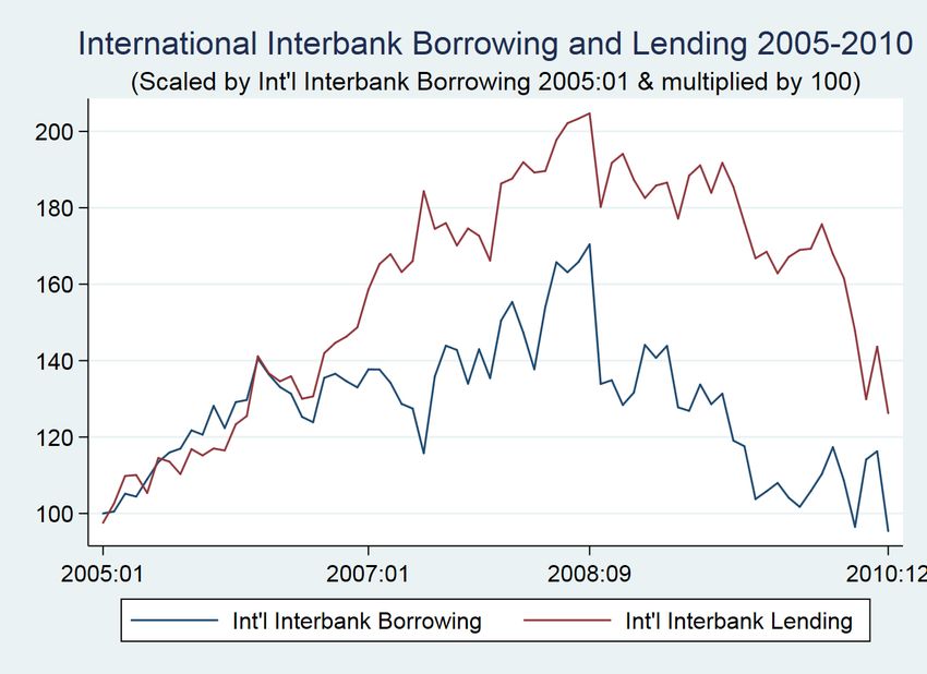
therefore additional credit line drawdowns during the crisis. As an exogenous proxy for the effect
of the crisis on a bank’s capital position, we use the bank’s pre-crisis exposure to US asset markets.
Using confidential data at the individual bank level, we show that banks with higher US asset
exposure at the onset of the crisis experienced larger US-related and also total asset value losses in
2008-09. Since such losses have to be marked to market, they directly affect a bank’s capital buffer.
Our proxy is in the tradition of the literature to use ex-ante asset holdings to capture ex-post losses
during crisis times (see e.g. Popov and Van Horen, 2015; De Marco, 2018; Acharya et al., 2018;
Ongena et al., 2018). Furthermore, the proxy is in the spirit of Peek and Rosengren (1997), Puri
et al. (2011) and Ongena et al. (2018) since it exploits an exogenous shock occurring in a distant
country.
We also expect that the more a bank depended on wholesale funding before the crisis, the more
sensitive it was to additional credit line drawdowns in 2008-09. This is because it faced a larger
shock to its cost of liquidity and thus the cost of meeting additional credit demand from its firms.
To proxy for this type of crisis exposure, we follow Ongena et al. (2015) and use a bank’s pre-crisis
dependence on international interbank funding.

Controlling for firm-specific changes in credit demand and creditworthiness (Khwaja and Mian,
2008), we find that banks with a one standard deviation larger US asset exposure significantly
cut little-used credit lines by 12 percent and more than other banks between January 2008 and
December 2009. What’s more, we show that US-exposed banks that had a relatively small capital
buffer at the onset of the crisis cut little-used credit lines more than US-exposed banks with a
relatively large buffer. Our interpretation of these results is that banks with a distressed capital
position during the crisis cut little-used lines mostly as a precautionary move to limit further capital
problems. This conclusion is supported by our finding that among little-used lines, those that had
a larger commitment volume and therefore posed larger risk to a bank’s capital buffer were cut
significantly more. In addition to reducing risk, banks may have also cut little-used lines to free
capital directly, although the resulting effect is limited because the capital charge on the unused
portion of most credit line types has been small (see Section 3). Our results also indicate that
banks with a distressed capital position did not cut credit lines that were used more intensely than
the median credit line. We conclude that this is because they posed a smaller risk of additional
drawdowns and because banks wanted to avoid imposing credit constraints on their firms. The
latter was arguably a good strategy to limit payment defaults of firms and to prevent firms from

                                                   4
switching to other banks in the short, medium or long run, especially given the importance of rela-
tionship lending in Austria. These concerns were clearly smaller when banks cut little-used lines,
while at the same time it enabled banks to reduce the risk of a sudden capital ratio reduction in
times in which capital was scarce and expensive.
We also find that a one standard deviation increase in pre-crisis dependence on international inter-
bank funding lead to a substantial reduction of little-used credit lines by up to 18.5 percent over
2008-09, controlling for a bank’s US asset exposure and initial capital buffer. Again, the impact
was larger than for other banks, and highly-used lines were not significantly cut. We also show
that conditional on Similar to our results on the “capital channel”, this shows that banks actively
reduced the risks caused by undrawn credit lines, but that this implied a substantial transfer of
liquidity risk to the corporate sector.
Our main set of results provides an additional rationale for the policymaker’s quest to ensure that
banks have a sufficiently large capital buffer. What’s more, our findings may reflect that the regula-
tory framework prior to the crisis induced banks to excessively grant credit line volumes that could
not be sustained in crisis times, when both the risk and the consequences of additional drawdowns
increase. In this light, the measure of Basel III to increase the capital charge on unused credit lines
compared to Basel II may smoothen credit line supply over the business cycle in the future. This
would limit the impact of runs on undrawn credit lines on banks. Similarly, the introduction of
the Liquidity Coverage Ratio (LCR) in Basel III, which requires banks to hold an adequate stock
of unencumbered high-quality liquid assets, may better prepare banks for liquidity problems and a
rise in credit line demand. Both the higher capital charge on unused credit commitments and the
LCR might therefore soften the magnitude of liquidity risk transfers from banks to firms in periods
of financial distress.
2 Contribution to the literature
We empirically establish a link between bank capital requirements and credit supply in light of the
regulatory treatment of unused credit commitments. To the best of our knowledge, the only study
that has directly addressed this relationship before ours is a mainly theoretical and yet unpublished
contribution by Foote (2011). This paper shows that the low capital charge on unused credit com-
mitments in the Basel regulatory framework induces banks to offer larger credit line volumes than
5it would optimally grant if the capital charge were as high as it is for the used portion of a credit
commitment. This creates misallocation of credit during credit market turmoil, since troubled firms
then draw heavily on existing credit lines and thereby constrain the bank’s ability to grant new
credit. In her empirical section, Foote shows that the ratio of undrawn credit lines over regulatory
capital negatively affected a bank’s origination of new credit during 2008-2009. However, she is
unable to control for selection issues. We add to this study by showing that over a horizon that
permits to adjust or abandon commitments, banks reduce their exposure to existing credit lines
that were perhaps granted excessively earlier, while accounting for selection issues. Our result that
banks cut little-used lines may partially reflect an attempt to reduce the misallocation described
by Foote. However, our finding that banks with a relatively small capital buffer cut little-used
credit commitments by significantly more suggests that this was (also) a move to mitigate capital
concerns.
Our paper also relates to a small literature that has dealt with asset-backed commercial paper
(ABCP) conduits (often called “shadow banks”) and their implications (Acharya et al., 2013;
Acharya and Schnabl, 2010; Covitz et al., 2013). This is because assets held by ABCP conduits
fully come on the balance sheet of the bank that set up the conduit only if liquidity guarantees on
these assets are used, which then decreases the bank’s capital ratio.1 More generally, our results
confirm that bank capital is an important determinant of bank lending behavior (Gambacorta and
Mistrulli, 2004; Berrospide and Edge, 2010; Gambacorta and Shin, 2016). We also corroborate
the finding that banks actively adjust their credit supply as a response to changes in net worth
due to exposure to certain assets and asset markets (Santos, 2010; De Haas and Van Horen, 2012;
Popov and Van Horen, 2015; De Marco, 2018; Ongena et al., 2018; Acharya et al., 2018). Regard-
ing capital regulations, we relate to a recent study by Gropp et al. (2018). This paper finds that
banks respond to an increase in their minimum capital requirement by reducing their risk-weighted
assets – including lending to the real sector – rather than raising their levels of capital. Our results
further confirm the results of the literature on macro-financial feedback loops, which suggest that
well-capitalized banks cut back assets and loans less than poorly-capitalized banks as a response
to adverse capital shocks (Brunnermeier and Sannikov, 2014; Brunnermeier et al., 2016; Farhi and
Tirole, 2017).
1
The implications are substantial and have concerned policymakers, as a citation in the IMF 2008 Financial
Stability on liquidity lines to ABCP conduits highlights: “Using the standards of Basel I, Fitch Ratings (2007)
estimated that, under a worst-case scenario, if liquidity lines were to be fully drawn down, declines in the
Tier 1 capital ratio of European banks would peak at 50 percent and for U.S. banks at almost 29 percent”.
(International Monetary Fund, 2008, p.77)
6Our findings also add to a growing literature that deals with liquidity risk caused by unused credit
commitments. Several studies have shown that deposit funding can help to mitigate this risk
(Kashyap et al., 2002), especially during periods of tight liquidity (Gatev et al., 2009; Gatev and
Strahan, 2006). Acharya and Mora (2015) highlight that in the US, banks were only able to honor
credit line drawdowns during 2007-2009 because of explicit and large support from the government
and government-sponsored agencies. Ippolito et al. (2016) find that the likelihood of Italian firms
to draw down previously unused credit lines during the interbank market freeze in the summer of
2007 increased with the dependence on interbank funding of their banks. However, exposed banks
did not significantly reduce credit line volumes, despite higher funding costs. This is arguably due
to the fact that unless the borrower violated a covenant, most credit lines could not be adjusted
downwards over a period of only two months even if the bank had wanted to. Given our horizon
of almost two years, this is different in our setting. Ippolito et al. (2016) also show that banks
that were more exposed to liquidity shocks actively managed this risk ex ante by granting fewer
credit lines to firms that were expected to draw down unused credit lines more extensively during
crisis times. We confirm this result by showing that firms that held little-used credit lines had a
significantly lower probability of default before the crisis (see section 5.5). Ivashina and Scharfstein
(2010) document a run on credit lines in the US after the Lehman default and find that banks
responded to this drain on liquidity and higher funding costs by reducing new lending. Cornett
et al. (2011) find that banks with higher levels of unused credit commitments managed the resulting
liquidity risk by increasing their liquid asset holdings and by reducing new credit origination during
2007-2009. We mainly contribute to this liquidity-oriented literature by showing that banks not
only take action outside of their credit line portfolio conditional on liquidity risk due to unused
credit lines, but also actively limit this risk itself by reducing their exposure to undrawn credit
commitments.
In a broader sense, our study relates to the literature on the effect of liquidity shocks on credit
supply to firms without explicitly focusing on credit commitments (Khwaja and Mian, 2008; Schn-
abl, 2012; Iyer et al., 2014; Allen et al., 2014; Cingano et al., 2016). We contribute to this body
of work by showing that while financial distress does not necessarily imply a reduction in actual
loan volumes, it can reduce the amount of credit firms can at most obtain from banks. This is
equivalent to a transfer of liquidity risk from banks to firms, a phenomenon that has received little
attention so far. Last, but not least, our paper adds to the theoretical (Boot et al., 1987; Martin
7and Santomero, 1997; Holmström and Tirole, 1998; Acharya et al., 2014) and empirical (Sufi, 2009;
Berger and Udell, 1995; Shockley and Thakor, 1997; Agarwal et al., 2006; Demiroglu and James,
2011) literature that specifically analyzes the nature, motivation and use of credit commitment
contracts.
3 Background and Data
Credit lines and Basel capital regulations
Basel I and II have requested banks to hold capital worth at least eight percent of their risk-weighted
assets. Independently of the risk associated with a credit commitment, the used portion and the
unused portion of the commitment do not equally enter risk-weighted assets in this framework.
The used portion obtains a ‘credit conversion factor’ (CCF) of 100%, which implies that it fully
enters risk-weighted assets. The unused portion in turn has only obtained a CCF of at most 50%
in the different versions of the Basel regulatory framework. This implies that a rise in the usage
of the credit commitment triggers an increase in risk-weighted assets for the granting bank and
thus a reduction in its capital ratio, unless the bank raises additional capital. The specific CCF
of the unused portion of a credit commitment depends on the type and maturity of the credit
commitment and has changed over time. Under Basel I, the unused portion of an irrevocable credit
commitment with original maturity below one year had a CCF of zero percent and was thus fully
off-balance-sheet, while those with maturity greater than one year had a CCF of 50%. A credit
line is irrevocable if its volume cannot be reduced before the commitment matures unless the firm
violates a covenant. With Basel II, which was fully implemented in January 2008 and was the
applied framework over our entire sample period, the CCF on irrevocable credit commitments with
maturity below one year increased to 20%. The CCF on long-term irrevocable commitments re-
8mained at 50%.2 Revocable commitments, which are unconditionally cancellable by the bank at
any time, had no capital charge in both Basel I and II. This is despite evidence that banks mostly
honor such commitments in adverse conditions to avoid losing reputational capital (Bhalla, 2008,
see p.407). In the credit commitment regulations of Basel III which were introduced in 2013, ir-
revocable commitments have faced a charge of 40% irrespective of their maturity while revocable
commitments have had a CCF of 10%.
Bank capital and the crisis in Austria
Austrian banks suffered a deterioration of bank capital ratios due to losses during the crisis (Schürz
et al., 2009). This was especially problematic since for Austrian banks raising additional capital
has been difficult. Specifically, Austria’s Financial Market Stability Board (FMSB) has argued that
“central risks for the Austrian banking system emanate (...) from banks’ specific ownership struc-
tures, which would not fully ensure the adequate recapitalization of banks in the event of a crisis”
(FMSG, 2017). The background is that many Austrian banks are part of a banking group, which
makes it difficult for a specific group member to raise capital from financial markets without dilut-
ing the equity share of other members. Making things worse, Austrian banks already had relatively
low capital buffers as they entered the crisis (Fonseca and González, 2010). These factors possibly
contributed to the weak stock market performance and large CDS spreads of Austrian banks in
2
In January 2007, the standardized approach and the foundation internal rating-based approach (F-IRB) of Basel
II became applicable, while the advanced internal rating-based approach (A-IRB) could be applied from January
2008 onwards (Musch et al., 2008; Deutsche Bundesbank, 2009). The CCFs indicated in the main text apply
only to the standardized and F-IRB approach. In the A-IRB approach, banks estimate CCFs themselves, at the
individual credit commitment level. Among other factors, this is done based on past usage-to-granted volume
ratios. This implies that on average, also in the A-IRB approach unused commitments must be backed with less
capital than used commitments, which is what ultimately motivates our research question around the “capital
effect”. Only some of the very largest banks operating in Austria have adopted the A-IRB approach. Those
banks face a trade-off. While cutting little-used credit commitments reduces the risk of sizable drawdowns, it
also raises the usage-to-granted volume ratio of the commitment, which leads to an increase in the commitment-
specific future CCF. Banks that apply the A-IRB approach thus might have a larger incentive not to cut credit
commitments than banks applying the standardized or F-IRB approach, conditional on a given current CCF.
This “works against us” in finding a negative effect of capital concerns on credit line supply and is therefore not
a major concern in terms of identification.
92008-09 (see Figure 2).3 4 This development occurred despite the Austrian banking package, which
“helped prevent a liquidity squeeze and expand banks’ capital buffers” (Schürz et al., 2009, p.56).
The weak stock market performance in turn reduced the amount of capital that could be raised
at the expense of a given loss of (perhaps voting) equity and thus aggravated the institutional
problems caused by the design of many banking groups. These considerations imply that Austrian
banks were particularly sensitive to a reduction in their capital ratio and thus additional credit line
drawdowns during the 2008-09 financial crisis.
Measuring US asset exposure
We use a bank’s pre-crisis holdings of US assets over total assets as a proxy for how the capital
position of a bank operating in Austria was affected by the crisis. The data comes from the Aus-
trian Central Bank’s database of individual bank balance sheets. Pre-crisis US asset holdings are
arguably the “cleanest”, i.e. most exogenous proxy for incurred losses. This is because the origins
of the crisis lied in the United States and were not related to the Austrian banking sector. We
measure US assets over total assets as the sum of securities and equity shares acquired from US
counterparties and loans to US counterparties divided by the sum of a bank’s total loans, securities
and equity shares, in December 2006.5 In line with previous studies, this moment of time is chosen
well ahead of the crisis.6 Importantly, US assets as we measure them may be denominated in any
currency, not only in US dollars. At the same time, assets for which the direct counterparty is not
located in the United States are not included in our measure.7 Although US assets only constituted
3
Supporting evidence for this claim is provided by Demirguc-Kunt et al. (2013), who study a multi-country panel
of banks and find that a stronger capital position was associated with better stock market performance during
the crisis.
4
Another reason for the weak stock market performance of Austrian banks was their exposure to the CESEE
region, whose performance was regarded as uncertain by financial markets at the time. The average Austrian
bank’s exposure to CESEE assets clearly exceeded its US assets exposure and triggered substantial news coverage
during the crisis. Nonetheless, for two reasons we do not choose CESEE exposure to proxy for the effect of the
crisis on a bank’s capital position. First, it must be doubted that losses in the CESEE region that affected the
capital position of banks operating in Austria were purely a result of the global financial crisis and in this sense
exogenous to the Austrian banking sector. Second, while pre-crisis CESEE asset holdings are associated with
larger CESEE-related losses during 2008-09, they do not significantly correlate with total net asset value gains
over the same time period. This makes CESEE asset holdings a worse predictor of total losses than US asset
holdings. Nonetheless, we do feature CESEE exposure as a control variable in our empirical analysis; see section
4.
5
On the average balance sheet of the banks in our sample (weighted based on the frequency of the bank in our
sample), 50 percent of US assets were securities, 49 percent were loans and one percent were equity shares in
December 2006.
6
This avoids for example to classify a bank that sold off its US assets with losses as the crisis began to unravel
in 2007 as not exposed to the crisis.
7
This implies that if an Austrian bank buys a security that was issued in the United States from a German bank,
then the security is classified as a German security, since the direct counterparty is German.
10one percent of (non-risk-weighted) total assets of the average bank in our sample, they made up
13.6 percent of capital and almost half of a bank’s capital buffer in December 2006 (see Table 1,
panel II).8 These statistics should be taken as a lower bound of the actual exposure to US asset
markets, given that only direct counterparties are considered. Using confidential data at the bank
level, we are able to track the distribution of US asset-specific value gains and losses due to changes
in market values over time (see Figure 3). We show in section 5.3 that for the average bank, larger
pre-crisis US asset holdings were significantly associated with larger US-related losses and also
larger total losses during 2008-09. In September 2008 alone, the month of the Lehman default, US
asset write-downs on average wiped out around five percent of the average bank’s capital buffer.
Since these losses have to be marked to market, they imply a smaller buffer towards the bank’s
regulatory minimum capital requirement. Figure 3 shows that also the volatility of net US asset
value gains was elevated from 2007-09, which suggests increased uncertainty about the value of
US asset holdings during the crisis.9 Taken together, these results suggest that pre-crisis US asset
exposure is not only an exogenous but also economically relevant proxy for capital losses of banks
operating in Austria during the Great Recession.
The extent to which capital losses affected a bank’s credit line management probably also depended
on the bank’s initial capital buffer. Therefore, we use confidential supervisory data to incorporate
this variable into our analysis. We compute a bank’s capital buffer as the ratio of its Tier 1 +
Tier 2 capital holdings and the bank’s corresponding minimum capital requirement. This variable
is a more precise indicator of how well a bank can absorb capital losses than bank capital over
total assets, which does not take the riskiness of a bank’s asset portfolio into account. In terms of
timing, we compute a bank’s capital buffer as of the end of the first quarter of 2008 in order to take
into account the regulatory changes that came with the full implementation of Basel II in January
2008.10
Liquidity problems during the crisis in Austria
The 2008-09 financial crisis was also a crisis of liquidity. For example, the cost of unsecured inter-
8
We use weights to compute the descriptive statistics in panel II of Table 1. The weight of each bank equals its
share in the number of credit lines in our sample. The results are similar when we use a bank’s share in the
total credit line volume in our sample as weight.
9
The actual uncertainty was arguably still higher than Figure 3 suggests, since the valuation of assets whose
market completely dried up was often done using bank-internal models (Ellul et al., 2014).
10
Our results are robust to choosing the last quarter of 2006, which parallels the timing of our other bank-specific
independent variables; see section 5.3.
11bank funding increased sharply with the Lehman default (see Figure 4). This was mainly driven
by a sharp increase in perceived counterparty risk, and lead to a reduction in the volume of unse-
cured interbank deposits on a global scale. It was difficult for banks to fully substitute interbank
funding with other sources of finance during the crisis. The cost of issuing bonds increased and the
sudden nature of the crisis made it impossible to increase retail deposits quickly (Brunnermeier,
2009). In the wake of these events, Austria’s eight-largest bank at the time, Kommunalkredit AG,
suffered an acute liquidity crisis and was subsequently taken over by the Republic of Austria under
the interbank market support and financial markets stabilisation act in November 2008 (Moody’s
Investors Service, 2010).
Measuring dependence on interbank funding
As Figure 5 shows, banks operating in Austria continuously reduced both international interbank
lending and borrowing after a peak in late 2008, which shows that they were feeling the repercus-
sions of the higher interbank funding rates. Given this evidence, we adopt pre-crisis dependence on
interbank funding as our proxy for bank-specific exposure to wholesale funding and thus exposure
to higher liquidity costs during the crisis. Following Ongena et al. (2015), we measure dependence
on interbank funding as total international interbank borrowing divided by total assets on the
bank’s balance sheet. We do so since Austria is a relatively small economy and domestic pre-crisis
interbank borrowing within, but also outside of the banking group is arguably a poor proxy for
exposure to increased liquidity cost in the aftermath of the Lehman default. Again, we choose
December 2006 as our point of measurement. As Table 1, panel II shows, the (weighted) average
of international interbank borrowing over total assets in this month across the banks in our sample
was 9.8 percent.
The Austrian Credit Register as primary data source
Our source of credit data is the Austrian credit register. The register documents all bank-firm credit
relationships in a given month as long as the offered credit volume or usage exceeds e350,000.11
11
Credit usage may exceed the commitment volume since overdrawing may be possible.
12This threshold implies that we study credit supply to medium-sized and large firms.12 Our sample
includes foreign banks but does not contain firms outside of Austria.13 While Austrian banks are
often organized in groups, credit decisions are typically made at the individual bank level, which
is why our unit of observation is a bank-firm relationship.
What we observe for such a relationship is the sum of all credit commitments the bank grants to
the firm in a given month. This sum can include revolving credit lines but also other types of credit
such as term loans. However, for all individual credit types the granted amount may exceed the
firm’s actual usage and this also frequently occurs in the data in later years in which commitment
data by credit type is available. Therefore, we treat a bank’s total credit commitment to a firm
as one bank-firm specific credit line in our analysis. Bearing this in mind, we interchangeably use
the terms ‘credit commitment’ and ‘credit line’. Our main dependent variable is the change in this
variable at the bank-firm level between January 2008 and December 2009. When evaluating this
change in our empirical analysis, we always control for the initial relevance of the distinct types of
credit at the bank-firm level. This is possible since we observe usage by credit type, and is impor-
tant because the initial usage composition may affect the change in the credit commitment volume
over time. On average, we observe a reduction in credit commitments by 4.5 percent over our
sample period (see Table 1, panel I). The choice of January 2008 as beginning of our sample period
comes at the cost of disregarding potential credit line reductions based on early crisis warning signs
in 2007. However, it avoids to pick up the effect of regulatory changes across Basel I and II, which
was fully implemented only in January 2008. December 2009 is chosen since lending standards and
credit volumes continuously tightened from the borrower’s perspective until the end of 2009 (see
Figure 1) and due to a change in reporting requirements with January 2010 that affected the credit
register variables.
For each bank-firm-pair, we compute the ratio of total credit usage and credit commitment vol-
ume in January 2008. We then compute the median of this variable across all pairs, and refer
to the commitments that are used less than median as ‘little-used credit lines’ and to the rest as
12
Table 1, panel III contains summary statistics on firms included in our sample, as of 2007. We only have firm-
specific data for 74 percent of firms that appear in the sample of credit lines of our main specification for the year
2007. This is because not all firms are required to send their balance sheet to the Austrian Central Bank, and
not all remaining firms follow the invitation to send it voluntarily. However, this is a relatively minor issue since
we only rely on firm-specific data in one auxiliary regression (see Table 9). Also from a conceptual perspective,
the fact that small Austrian firms are therefore underrepresented in our sample is a small problem. The reason
is that larger firms have larger credit lines and thereby banks are more likely to undertake active credit line
management with large firms, as we show in section 5.3 for details.
13
We track bank mergers, split-ups, and bank identifier changes for other reasons over time in our analysis; see
the Appendix for details.
13‘highly-used credit lines’. The computed median equals 0.97, while the mean is 0.84. Both these
numbers are relatively close to one since it is possible and frequently occurs that credit lines are
“overdrawn”. Among little-used lines, the average ratio of usage to granted credit equals 0.557.
The average little-used credit line was cut by 9.9 percent between January 2008 and December
2009, while the average highly-used line was increased by one percent. The total unused volume of
granted credit commitments makes up 3.1 percent of assets of the average bank in our sample.
4 Empirical Strategy
We start our empirical analysis by analyzing the effect of US asset exposure and dependence on
interbank funding on credit line supply during the crisis irrespective of how much credit lines were
initially used. As an initial exercise, we also study the differential treatment of little-used lines by
the average bank. To do so, we set up the following specification:
∆log(CreditLineij ) = α1 U SAssetsj +α2 Interbankj +α3 Bj +α4 Little-usedij +α5 Cij +ηi +ij (1)
∆log(CreditLineij ) approximates the percentage change in the credit commitment volume offered
by bank j to firm i between January 2008 and December 2009. USAssetsj is the bank-specific
ratio of US assets to total assets and Interbankj the bank-specific ratio of international interbank
borrowing to total assets in December 2006. Bj is a vector of bank-level controls that may have
affected credit supply during the crisis and are likely to be correlated with US asset exposure and/or
dependence on interbank funding. Contrary to equation (1), in later specifications that address our
main research questions we will be able to replace this vector with bank fixed effects. Bj includes
bank size as measured by log total assets, a bank’s liquidity ratio, capital to asset ratio, return on
assets, loan write-offs over total assets and CESEE assets over total assets, and are measured at
the latest possible time in 2006.14 All bank-specific variables are scaled by their standard devia-
14
While CESEE assets over total assets is an important control due to the exposure of some Austrian banks to
the region, the prior variables are standard in the literature. The liquidity ratio is measured in December 2006
and computed as the ratio of cash and balance with central banks plus loans and advances to governments and
credit institutions divided by total assets, following Jiménez et al. (2012). As Iyer et al. (2014) point out, a high
liquidity ratio helps to absorb subsequent liquidity shocks. Return on assets (ROA) are measured as net income
over average total assets in 2006. ROA and capital over assets, which is measured in December 2006, capture
the ability of banks to take risk and absorb losses during a crisis (Cingano et al., 2016). Loan write-offs are the
total as of 2006 and capture whether banks were making losses at the onset of the crisis and thus may have
been particularly sensitive to shocks during the crisis (Santos, 2010). Total assets are measured in December
2006. The same holds for CESEE assets, which are defined analogously to US Assets but focus on 22 countries
in central, eastern and southeastern Europe. See the Appendix for a complete list of included countries.
14tion.15 Little-usedij is a bank-firm-specific dummy variable that equals one if the ratio of credit line
usage to the granted volume is below the median in our sample. α4 thus indicates the differential
treatment of little-used versus highly-used credit lines of the average bank during the crisis. In
our preferred estimation of α4 , we replace our bank-specific variables by bank fixed effects. This
allows to control for all confounding factors that affected a specific bank’s change in credit supply
between January 2008 and December 2009.
The vector Cij contains bank-firm-specific variables. These include the share of bank j in total
credit usage of firm i, the duration of the credit relationship and a set of dummy variables that
indicate the type(s) of credit commitment(s) granted by bank j to firm i. All bank-firm-specific
variables are measured in January 2008.16 We cluster standard errors at the firm and bank level
to account for possible serial correlation of errors within these groups.
Importantly, not only supply factors influence a bank’s credit line management, but also firm credit
demand and creditworthiness. These variables are likely to vary over time, especially across normal
and crisis times. We take this into account by restricting our sample to firms that borrowed from
multiple banks in both January 2008 and December 2009 and including the firm fixed effects ηi
into our specification (Khwaja and Mian, 2008). While this results in dropping 50% of firms from
our sample, credit commitments to these single-bank firms only made up 17 percent of the total
commitment volume in January 2008. This is partly because single-bank firms are smaller and have
credit lines that are smaller in volume. The omission of these firms is therefore not a big issue since
for a given ratio of credit usage to commitment volume, large credit lines have a greater potential
to cause a non-negligible capital ratio reduction and imply larger liquidity risk.17 The firm fixed
effects absorb all factors that are specific to the firm and lead to a change in its granted credit
commitment volume between January 2008 and December 2009.18
Conditional on the inclusion of firm fixed effects, there is one remaining identification assumption
15
This standard deviation is measured based on the sample of credit lines, thus banks that granted more credit
lines over our sample period obtain a larger weight in the computation.
16
Relationship duration is censored at 97 months since credit register data are only available to us from January
2000 onwards. Volumes by credit type are only recorded in terms of usage rather than the granted amount in
the credit register over our sample period. Specifically, total credit usage in a given month is reported both as a
sum and as of the following individual components: revolving loan, term loan, titrated loan, leasing loan, special
purpose loan, transmitted loan, liability. We include a dummy variable for each of these categories (except
revolving loan, which serves as the baseline category) which equals one if the usage of the respective credit line
type is greater zero in January 2008.
17
In section 5.3, we show that large little-used credit lines were cut more than small little-used lines by troubled
banks during the crisis, both in absolute as well as in percentage terms. This supports our argument that small
credit lines are less relevant for banks in terms of capital and liquidity management.
18
Therefore, they also control for seasonality factors that might affect a firm’s change in credit demand between
a January and a December.
15that must hold for an unbiased estimation of α1 and α2 . Specifically, it must be that a firm does
not disproportionally demand more or less credit during the crisis from those of its banks that are
particularly strongly or weakly exposed to capital and/or liquidity problems during the crisis. This
assumption would fail for example if firms first approached their relationship lender for a credit
line adjustment, while banks that focus on the business model of relationship lending have higher
US exposure or depend more on international interbank funding than the average bank. To test
whether such issues might bias our results, we feature a series of robustness checks on our main
findings in section 5.3.
4.1 Do troubled banks treat little-used credit lines differently?
Given our research questions, we have a special interest in credit lines that were used relatively
little at the onset of the crisis. Since banks whose capital or liquidity position was particularly
harmed during the crisis were more sensitive to additional drawdowns, we expect those to treat
little-used lines differently than other banks. We therefore interact both US Assets and Interbank
with the dummy variable Little-usedij . The resulting specification looks as follows:
∆log(CreditLineij ) = β1 U SAssetsj + β2 Interbankj
+β3 [U SAssetsj × Little-usedij ] + β4 [Interbankj × Little-usedij ]
+β5 Little-usedij + β6 Bj + β7 Cij + ηi + ij (2)
β1 indicates the effect of an increase in US asset exposure by one standard deviation on the bank’s
change in the granted credit line volume of an initially highly-used line, while β1 + β3 + β5 indicates
the effect on an initially little-used credit line. If β3 is statistically significant, then this provides
evidence that how differently a given bank treated little- versus highly-used credit lines in its
portfolio during the crisis depended on its US asset exposure, and thus arguably its capital position
during the crisis. A significant and negative β3 would thus support our hypothesis that capital
concerns affected a bank’s credit line management during the crisis.
The interaction terms in equation (2) allow to replace the non-interacted bank variables with
bank fixed effects. This has one conceptual disadvantage – which is why we start by estimating
equation (2) – but has a key methodological advantage, which is why we also estimate the following
specification:
16∆log(CreditLineij ) = β3 [U SAssetsj × Little-usedij ]
+β4 [Interbankj × Little-usedij ] + β5 Little-usedij + β7 Cij + ηi + δj + ij (3)
The described advantage of including the bank fixed effects δj is to control for unobserved bank-
specific factors that affected the change in credit line supply between January 2008 and December
2009. Intuitively, adding bank fixed effects implies that we analyze how little- versus highly-used
credit lines are treated within a certain bank. The mentioned cost of their inclusion is to make it
impossible to estimate the absolute effects β1 + β3 + β5 and β2 + β4 + β5 . Instead, they only allow
the estimation of the relative effects β3 + β5 and β4 + β5 . For example, β3 + β5 indicates the effect
of an increase in US asset exposure on the change in the granted credit line volume of a little-used
line relative to a highly-used line.19
In order to create a stronger test whether a bank’s credit line management during the crisis was
influenced by capital considerations, we account for the bank’s capital buffer at the onset of the
crisis. We do so by interacting the interaction of US Assets and Little-used with a variable that
equals one if the ratio of the bank’s regulatory capital over its minimum capital requirement in
January 2008 was below the median. This median equals 1.62.20 For the test we have in mind,
it is sufficient to understand whether the effect of US asset exposure on the management of little-
used lines relative to highly-used lines depends on a bank’s capital buffer. Therefore, our main
corresponding specification builds on specification (2), and looks as follows:
∆log(CreditLineij ) = γ1 [U SAssetsj × Little-usedij ]
+γ2 [U SAssetsj × Little-usedij × SmallBuf f erj ] + γ3 [Little-usedij × SmallBuf f erj ]
+γ4 [Interbankj × Little-usedij ] + γ5 Little-usedij + γ6 Cij + ηi + δj + ij (4)
γ1 + γ2 + γ3 indicates the effect of an increase in US asset exposure by one standard deviation on
the change in the granted volume of a little-used line relative to a highly-used line if the bank had
19
β3 + β5 thus provides less information than β1 + β3 + β5 ; for example, β3 + β5 would be negative and significant
even if US-exposed banks with a low capital buffer increased the granted volume of little-used credit lines in their
portfolio during 2008-2009, but increased the supply of highly-used credit lines significantly more. However, if
that were the case, then β1 + β3 + β5 would be positive and thereby reveal that little-used lines were actually
increased in an absolute sense.
20
We build this median in such a way that it is not the median across banks, but across observations of the sample
of our main specification, such that the number of credit lines associated with Small capital buffer = 1 is equal
to the number of credit lines associated with Small capital buffer = 0. Since banks that have a relatively small
capital buffer grant more credit lines in our sample, the subsample for which Small capital buffer = 1 includes
109 banks, while the subsample for which Small capital buffer = 0 includes 204 banks.
17a relatively low capital buffer. If γ2 is significant, then this strengthens our interpretation that US
asset exposure matters for a bank’s credit line management because of its capital position during
the crisis.
5 Results
The results of estimating equation 1 are reported in Table 2. While in column 1 we omit firm fixed
effects to gauge the relevance of selection effects, column 2 shows the results estimated based on the
full specification. The results suggest that neither an increase in US asset exposure nor dependence
on interbank funding lead to a change in credit supply for the average credit line.21 The coefficient
estimates are stable across columns 1 and 2. This speaks against substantial heterogeneity in credit
demand or creditworthiness across banks with higher US asset exposure and/or interbank funding
dependence and other banks. Our results also show that the average bank significantly cut credit
lines that were used relatively little at the onset of the crisis by almost 15 percent compared to
highly-used lines. This coefficient estimate is very robust to replacing bank controls with bank
fixed effects.
5.1 Little-used credit lines and varying capital and liquidity problems: Differ-
ential effects
The results of Table 2 suggest that the average bank reduced its exposure to undrawn credit lines
over 2008-09. Since the consequences of additional drawdowns are more severe for banks with a
weaker capital position and/or a larger exposure to the liquidity dry-up during the crisis, we expect
that those banks would reduce this exposure by even more than the average bank. This hypothesis
is the motivation for the introduction of interaction terms in equations (2) and (3). The results
on these specifications are reported in Table 3. In columns 1 and 2, we only interact US Assets
with Little-used. This ensures that the interaction term captures the differential treatment of little-
used lines by banks with a relatively large US asset exposure and the coefficient on Little-used
indicates how little-used credit lines are treated by banks with relatively low US asset exposure,
21
The coefficients on our bank-specific control variables are largely intuitive. Banks with a higher capital ratio or
larger liquid asset holdings significantly increased credit supply or reduced it less compared to their counterparts.
The opposite holds for banks that had suffered more loan write-offs before the crisis and were more exposed
to the CESEE region, whose performance was regarded as uncertain by financial markets during the crisis.
Larger banks increased credit supply or reduced it by less compared to smaller banks, while a bank’s pre-crisis
profitability had no impact on its credit supply over 2008-09.
18holding other bank characteristics equal. The results in column 1 indicate that banks with an
additional US exposure of one standard deviation (and thus about one percent of total assets)
indeed significantly cut little-used lines more than other banks, specifically by almost six percent.
Overall, these banks significantly cut little-used credit lines by about 12 percent, as can be seen
from the marginal effects reported at the bottom of the table.22 This corresponds to a reduction of
around e1.3 million. The size and significance of the coefficient estimates is robust to controlling
for bank fixed effects (see column 2).23 Since the average ratio of usage to granted volume of lines
that we define as little-used equals around 56 percent (see Table 1, Panel I), the magnitude of the
reduction does not imply acute credit constraints on the average holder of a little-used credit line
borrowing from a bank with large US exposure even if the firm was fully using all its other credit
lines.
The positive and insignificant coefficient estimate on US Assets in column 1 suggests that banks
with larger US asset exposure did not significantly cut highly-used lines compared to other banks.
This reconciles the result of Table 2 that the average credit line was not significantly cut by US-
exposed or interbank-dependent banks compared to other banks. Our primary interpretation is that
highly-used lines posed a smaller risk of additional drawdowns and thus a reduction in a bank’s
capital ratio. Clearly, cutting highly-used lines would free capital and thus directly increase the
buffer vis-a-vis the regulatory requirement. However, this would arguably have large costs to the
bank. Specifically, it could increase the likelihood of payment defaults and relatedly, the potential
imposition of credit constraints on the firm could induce it to switch to other banks or sources of
credit in the short, medium or long run. The latter might pose a particular danger in a financial
system in which relationship lending plays an important role, as is the case in Austria.24 Last, but
22
The magnitude of any given marginal effect is simply the result of adding up the relevant coefficients. In columns
1, 3 and 5, these marginal effects are absolute in the sense explained in section 4: in columns 2, 4 and 6 these
effects are relative to highly-used lines.
23
When controlling for bank fixed effects, the estimated effect of an increase in US asset exposure by one standard
deviation on the volume of little-used lines relative to highly-used lines equals approximately -14.7% (see the
marginal effect displayed in column 2). Note that this reconciles the estimated ‘absolute’ marginal effect of
column 1, which can be seen from subtracting the effect of additional US asset exposure on highly-used lines
by the estimated relative marginal effect of column 2: 0.027 - 0.147 - = -0.12. This suggests that the specific
magnitude of the estimated ‘absolute’ effect of additional US asset exposure on the supply of little-used lines is
very robust to controlling for bank fixed effects.
24
As Table 2 reveals, banks with larger exposure to the CESEE region significantly cut credit commitments
compared to banks with smaller CESEE exposure. In order to better understand whether not only US-exposed
banks but banks that were affected by the crisis along other measures cut highly-used lines less than little-used
lines and thus whether banks avoided imposing credit constraints on their firms, we additionally interact CESEE
Assets with Little-used in equation (3). The results, which are available from the authors upon request, indicate
that indeed, CESEE-exposed banks cut highly-used lines by only 2.7 percent (compared to an effect of -5% for
the average credit line), and the coefficient is only significant at the 10% level. We further note that our baseline
results are largely robust to the inclusion of the additional interaction term.
19not least, it could contractually be more difficult to cut highly-used lines compared to little-used
lines.
In columns 3 and 4, we interact Little-used only with Interbank. Our results show that banks
with a larger ratio of international interbank borrowing over total assets significantly cut little-
used credit lines by around seven percent more than other banks. This confirms our hypothesis
that such banks are more sensitive to credit line drawdowns and shows that they successfully
reduced this risk. In columns 5-6, we interact Little-used both with US Assets and Interbank.
This makes the interpretation of the non-interacted dummy Little-used less straightforward, but
allows to simultaneously account for both the capital and liquidity channel and trace out their
relevance conditional on the other. The coefficient on the interaction term Interbank × Little-used
is very robust to this modification. However, the coefficient on US Assets × Little-used becomes
smaller in magnitude and loses significance. While this suggests that high US asset exposure and
large dependence on interbank funding often come hand in hand, it may also reflect that US asset
market exposure alone may not yet fully reflect the state of a bank’s capital position during the
crisis. Specifically, a bank with relatively large US asset holdings that suffers capital losses but
went into the crisis with a relatively large capital buffer may be able to absorb those losses more
easily than others and thus decide not to cut little-used lines. We test this hypothesis in the next
sub-section.
5.2 Accounting for a bank’s initial capital buffer
If concerns about the regulatory capital ratio affect a bank’s credit line management during crisis
times, then banks that have a smaller capital buffer vis-a-vis their minimum capital requirement
should be more worried about undrawn credit lines and may cut them by more than otherwise sim-
ilar banks. We explore this logic by distinguishing the cross-section of banks along their individual
capital buffer and incorporating this variable into our empirical analysis as described in section 4.
The results are reported in Table 4. Column 2 estimates specification (4), while column 1 esti-
mates the corresponding specification with bank controls instead of bank fixed effects. The triple
interaction of US Assets and the dummy variables Little-used and Small capital buffer is negative
and statistically significant in both specifications. This confirms our hypothesis that US-exposed
banks with a small capital buffer cut little-used lines by significantly more than those with a larger
buffer. The marginal effects at the bottom of the table actually indicate that a bank with higher
US exposure only significantly cut little-used credit lines if it had a relatively small capital buffer.
20You can also read