Catalogue of representative scales to visualize different coverages in Google Earth - IOPscience
←
→
Page content transcription
If your browser does not render page correctly, please read the page content below

IOP Conference Series: Earth and Environmental Science

PAPER • OPEN ACCESS

Catalogue of representative scales to visualize different coverages in
Google Earth
To cite this article: A C Tristán et al 2021 IOP Conf. Ser.: Earth Environ. Sci. 686 012038

View the article online for updates and enhancements.

                                This content was downloaded from IP address 46.4.80.155 on 09/09/2021 at 07:49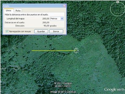
The International Conference on Smart and Innovative Agriculture                                               IOP Publishing
IOP Conf. Series: Earth and Environmental Science 686 (2021) 012038                        doi:10.1088/1755-1315/686/1/012038

Catalogue of representative scales to visualize different
coverages in Google Earth

                     A C Tristán1*, O R Cárdenas1, E J T Garza2, A G R Alvarado3, R F Putri4*, and
                     J Thio4

                     1
                       Facultad de Ingeniería, Universidad Autónoma de San Luis Potosí, San Luis Potosí,
                     México
                     2
                       Sacultad de Ciencias Forestales, Universidad Autónoma de Nuevo León, Linares,
                     México
                     3
                       Centro de Investigaciones Biológicas del Noroeste, S. C., La Paz, México
                     4
                       Department of Environmental Geography, Faculty of Geography, Universitas Gadjah
                     Mada, Indonesia
                      *
                          Corresponding author: abraham,cardenas@uaslp.mx, ratihfitria.putri@ugm.ac.id

                      Abstract. Representative scales were established, based on the zoom level of Google Maps,
                      for generating a catalogue of indicators from the scale-image relationship, into the Google
                      Earth visualization system. It was possible to analyze some functionalities of the visualization
                      system proposed, such as the depth of detail from image resolution and the images return.
                      Therefore, samples of four land use were analyzed. Furthermore, to associate the multilevel
                      mechanism of the visualization in Google Earth, a digital ruler was used as a tool that
                      measures the pixels per inch into the screen. In consequence, it is possible to analyze the
                      changing behaviour from one screen to another. With this, it is feasible to associate a specific
                      mechanism to improve the relationship between the handling of several images covering a
                      limiting territory, and the scales that best represents the themes described. Finally, 893 samples
                      were analyzed in 32 points of the territory, between the coordinates 14° to 33° N and 86° to
                      119° W. Finally, the error percentage, the variance, and the standard deviation were estimated
                      for determining the variation between the values calculated in different samples.

1. Introduction
Nowadays, many users of spatial technologies have associated to integrate vectorial mapping with
satellite imagery in universal server infrastructures, mainly in Google Earth, allowing research support
in the knowledge of territory elements [1-3]. Before the virtual globe development (visual system
development), web mapping showed significant alternatives for analysis and knowledge of the Earth.
For this reason, different programs, such as MapQuest, Google Maps and Map24, were popular for
some time [4]. On the other hand, Google Earth is an interactive visualization system that allows the
analysis of different types of images through depth mechanisms in image resolution [5]. The image
information is not related to a fixed scale so that we can find maps in several scales [6]. The
interoperability of Google Earth [7, 8], that has allowed the unification of data from different sources,
on several formats (.shp, .dwg, .fmw, among others), through its KML (Keyhole Markup Language)
structure [9], has enabled to develop millions of mapping operations through the GIS use, handling
              Content from this work may be used under the terms of the Creative Commons Attribution 3.0 licence. Any further distribution
              of this work must maintain attribution to the author(s) and the title of the work, journal citation and DOI.
Published under licence by IOP Publishing Ltd                          1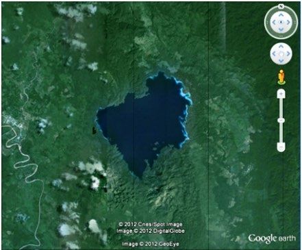
The International Conference on Smart and Innovative Agriculture                           IOP Publishing
IOP Conf. Series: Earth and Environmental Science 686 (2021) 012038    doi:10.1088/1755-1315/686/1/012038

data of various scales and integrate them to platform images [10]. Thus, we can get a better
appreciation of the vectorial data described on each territory based on its relationship with satellite
imagery [11]. Google Earth allows us to observe details due to the high resolution of its images [12].
However, it hasn’t been easy to measure certain inconsistencies of representation and description of
the objects, from vectorial data integrated with the variety of images that represent the territory, which,
have different resolutions and a multi-scale structure easy to handle but it has been complicated to
associate geometrical and topological correspondences [13].
    To observe and to analyze geographic objects, with a certain zoom level of the image, when
combined with vectorial data, it is difficult to obtain accurate integration because the vectorial data
come of a cartographic production to absolute scale [14]. In this way, the functionalities of Google
Earth and its mechanism scalar associated of the objects by a determined zoom [15] motivated this
work. It is interesting to study the relationship between elements or objects represented by different
images and the possible scalar representation of their structure — so we analyze the corresponding
part to Google Maps, as it has different views from ground level [16]. However, due that zooms are
not only fixed but constant, they depend on the area and the image resolution [17]. Likewise, each
zoom represents a scale, but its measure can have low precision depending on the resolution of the
image showed by Google Earth [18]. The representation of the information is presented through the
zoom, and this is associated with the increase or decrease of the objects focal distance [19]. The
zooming into an image in a computer multiplies the number of pixels that integrates, presenting larger
or smaller images on the screen despite the original object [20]. The scale, unlike the zoom, represents
a proportion value, and this is generally associated with a metric representation of the ground with the
graphical symmetry on a scale, a map, or a display system [21].
    To analyze cartographic scale in satellite images, cannot dispense some essential factors in which
the scientific community has worked hard, such that geometric accuracy and visual quality the image,
and its relation to scale by different criteria and standards for planimetric accuracy [22]. Considering
that different types of images from Google Earth that make Earth's description are subject to a UTM
projection system, these can be affected in their representation from latitude and longitude [23]. This
situation also affects several changes in determining the scale of the image, which to exert a zoom
degree in a specific area, generates a certain pixel increase in images that describe elements from the
territory. When the image resolution is lower, the latitude and longitude adapt to a series of
mechanisms of a little pixel representation. In such a way that it is possible to count through a specific
quantity of views, analysing the capacity to deepen in the image resolution, and the opposite process
of the zoom (go back). In this way, it is possible to associate the zoom levels with a determined scale.
    Likewise, it's necessary to consider the resolution of the screen where the elements analyzed of the
territory are observed, given that these screens are subject to specific pixel classifications, which are
converted automatically and adapted when viewing images of Google Earth on a particular type of
display. A mechanism developed [24], described in a patent (US 6,618,053 B1) "The asynchronous
multilevel texture pipeline" a method that reports real processes in which Google Earth structure
functionality is supported.
    The aim of this study is to generate a catalogue of scalar indicators in Google Earth for determining
the scale-image relationship that associates the characteristics that visually describe some elements of
land use. Additionally, it will facilitate knowledge of the image-scale relationship, for those who need
to determine distances, surfaces or volumes, and they take advantage of the resolution of the images
and their temporality.

2. Method
2.1 Study Area
The analysis will be performed with images covering the Mexican territory, between the coordinates
14° to 33° N and 86º to 119º W. Those images come from different sources: CNES/Spot, Digital
Globe, GeoEye, and NASA.

                                                     2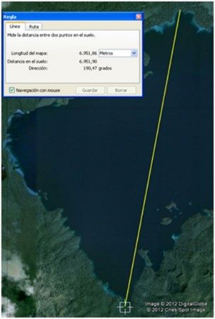
The International Conference on Smart and Innovative Agriculture                          IOP Publishing
IOP Conf. Series: Earth and Environmental Science 686 (2021) 012038   doi:10.1088/1755-1315/686/1/012038

2.2 Description of The Methodology
First, for selecting the samples, it will be generated a list of natural resources represented in the
Google Earth images. Then, a list of scales will be analyzed and determined in Google Maps, we will
relate them to the Google Earth interface, to associate specific correlation of scale representation.
Since the resolution of Google Earth images is defined by a factor known as pixels per inch (PPI).
This measure indicates the number of pixels that are in a physical inch on the monitor, so this is the
factor that causes a resized image from a screen to another due to the difference of PPI between both
screens. For sample measurement on screen, it will use JrulerPro software, which is developed by
Spadix Software Company. This tool is a digital ruler to measure any object on a screen. It's useful for
graph measurement and webspace distribution. The ruler can be displayed in pixels, inches, picas, and
centimeters. For this study, we used version 3.0 Pro. This ruler can be rotated, dragged, extended, and
change its graduation automatically, in addition to modifying its transparency.
    Initially, the procedure for determining relationships between scales and existing zoom levels in
Google Maps will be as follows: The Jruler software will be installed and once placed on the screen,
we enter into the zoom level to locate or focus on the country or city map of our choice, in this case,
will be placed in San Luis Potosi City, Mexico. Next, the map view mode changes, so we will
facilitate the measurement of do not have so many items on the screen. The zoom is fixed to the level
that we want to measure, this time we used as an example the 18-zoom level, to which we associate
the ruler. Thus, we can determine the number of pixels that measures the line from end to end, and we
obtain a measurement of about 90 pixels. As previously noted, the number of pixels from which an
image is formed varies depending on the screen resolution where it is located.
    By changing the Jruler adjustment in cm for measuring scale line again, it gives an approximate 2.5
cm scale line from end to end. Because Jruler automatically changes the number of pixels per inch, the
measurement will not change, no matter the screen or the resolution is displayed, the line always will
measure 2.5 cm. This line represents a 50 m measure or 5000 cm, but according to the ruler, it
measures 2.5 cm. If we divide the measure, that represents the line (5000 cm), by what it measured
(2.5cm), it will result in the centimeters proportion value of an estimated scale of 2000. The steps
indicated were repeated with each of the 20 zoom levels in Google Maps, to determine the equivalence
in centimeters between Jruler and zoom levels.

2.3 Experimentations with Sample Measurement in Google Earth
For associating the scales identified in Google Maps, we will proceed to establish a mechanism in
Google Earth. Subsequently, on a specific area of the image, the baseline will be drawn, trying to mark
the greater length in the element and then determined data are recorded in the ruler window. It should
be noted that this procedure involves determining criteria for measuring water bodies in which it was
intended to find a length and surface similarity between these elements represented in various images
of Google Earth. We also set a mark to obtain the sample coordinates; subsequently, an auxiliary line
is traced next to the object of analysis, to determine the scale.
    Also, we need to represent a line of 200 meters in 2.5 cm on the screen, for adjusting the zoom
view and reach the size measure of the auxiliary line. This procedure determines the scaling in the
view, after setting the zoom to the size of the auxiliary line. The view will be on the indicated scale
being able to be measured with Jruler. This procedure was repeated so many times over elements from
the same site, taking account the adequacy of Google Earth zoom, concerning those scales which
allowed to observe the sampling element, in the capacity for deepening in image resolution and its
opposite process (go back) of each image resolution in which the item was located.
    Then we will measure the indicated element, taking care not to change the zoom view, to measure a
baseline using Jruler. This operation allows us to work in the image position. From this image, the
zoom parameters are stated, and the length is obtained with the ruler at the determined view; thus, its
value is in centimeters. This value is multiplied by the meters represented on the scale line. Likewise,
the value of "height of the eye" is also taken, serving to determine the observed variations of each
view at different zoom levels. Each item considered will be based on the scales established for

                                                     3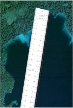
The International Conference on Smart and Innovative Agriculture                           IOP Publishing
IOP Conf. Series: Earth and Environmental Science 686 (2021) 012038    doi:10.1088/1755-1315/686/1/012038

associating with those objects that could be measured, these being visible on screen as an established
scale.

2.4 Sample Analysis of The Image-Scale Relationship
It will be obtained a representative scale set to handle the different Google Earth images. These scales
will be generated from the sample analysis, regarding the zoom functionality, within process deepen -
going back to each analyzed image resolution in various soil coverages. At this step, is associated that
for each selected topic exists a scales variety that is representative for handling the various images
covering the analysis sector in this work. However, there are full, considered implications in the use of
such scales determined for each subject, analysing procedures based on the description of error ranges,
depending on the analysis variety of each sample.
    To perform a comparison of the sample lengths obtained by measuring on each scale with Jruler
will be calculated the percentage error. This standardization will be made so that handle an error
range, so that, for each sample, it will be obtained the difference based on calculated length
measurement on the screen and the determined measure with the Jruler, which describes the error. The
error is multiplied by 100 and divided by sample length (measured with Jruler), giving an error
percentage in the determined scale.

2.5 Variation of Error in Each Scale
    Once the percentage of error between the length of the sample in the Google Earth interface has
been shown, what is obtained with the ruler, as well as their respective calculations, right away the
variations between the errors in each scale will be described (including the percentage of error). In this
case, both variables support to find a scale where there is greater variation among the errors, that is,
where the errors of the measurements are more likely to suffer more significant alterations. To analyze
such variations, we apply the following formula of variance (σ2) to measure the mean of the
differences between the set of error values in the different scales analyzed. Similarly, knowing how
much data are separated from percentages, the standard deviation was determined (σ) to measure
dispersion in the average of the distances between the error percentages determined.

                                               (1)                                (2)

 Where: s2= Variance; xi = Observed value; = Average of observations; n = The sample elements

3. Result and Discussions
3.1 Sample Selection
Initially, water, soil, agriculture, livestock, coastlines, flora, and fauna, infrastructure, communication
routes, urban and rural areas were selected. Then, the criterion of being able to capture in the images
the sharpness of the object and the shape of its typical characteristics was established to be able to
measure it to select the final coverages. Finally, the four covers selected were agriculture, bodies of
water, infrastructure, and forest. Likewise, a sample was chosen of each coverage in for each state of
the country, and which in turn was representative. States in which the selected coverages were not
observed were omitted. This procedure allowed us to establish the following scale catalogue at
different zoom levels (Table 1).

                                                     4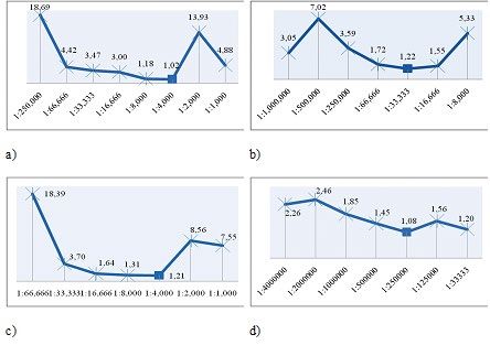
The International Conference on Smart and Innovative Agriculture                          IOP Publishing
IOP Conf. Series: Earth and Environmental Science 686 (2021) 012038   doi:10.1088/1755-1315/686/1/012038

         Table 1. Scales Associated with Google Maps According to Different Zoom Level
                    Linear meters        Centimeters measured     Proportion of centimeters
       Zoom
                     represented              with Jruler             in estimated scale
         0            10,000,000                   2                     1:500000000
         1             5,000,000                   2                     1:250000000
         2             2,000,000                   2                     1:100000000
         3             2,000,000                  3.2                     1:62500000
         4             1,000,000                  3.2                     1:31250000
         5              500,000                   3.2                     1:15625000
         6              200,000                   2.5                      1:8000000
         7              100,000                   2.5                      1:4000000
         8               50,000                   2.5                      1:2000000
         9               20,000                    2                       1:1000000
        10               10,000                    2                       1:500000
        11                5,000                    2                       1:250000
        12                2,000                   1.6                      1:125000
        13                2,000                    3                        1:66666
        14                1,000                    3                        1:33333
        15                 500                     3                        1:16666
        16                 200                    2.5                        1:8000
        17                 100                    2.5                        1:4000
        18                  50                    2.5                        1:2000
        19                  20                     2                         1:1000
   (Source: Data Measuring, 2020)
3.2 Experimentations with Sample Measurement in Google Earth
To associate the scales identified in Google Maps, we located the sample area according to the item or
object, representing a land use. In this case, as an example, we take a water body sample in Lake
Miramar (Figure 1) in the state of Chiapas. Next, we draw a line based on a specific area of the image,
marking the largest length of the element (Figure 2) and saving the obtained data in the ruler window.
It should be noted that this procedure involves determining criteria for measuring water bodies in
which it was intended to find a length and surface similarity between these elements represented in the
various images of Google Earth. In the following example (Figure 3), was fitted the view at 1:8000,
under the relation of scales defined in Table 1. Here, we drew a line of 200 meters with the Google
Earth ruler, which must correspond to the 2.5 cm measurement on Jruler.

Figure 1. Example of a water          Figure 2. Baseline definition          Figure 3. Auxiliary line
 body sample in the state of
                                                                                   definition
          Chiapas

                                                     5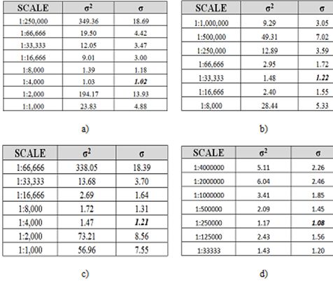
The International Conference on Smart and Innovative Agriculture                          IOP Publishing
IOP Conf. Series: Earth and Environmental Science 686 (2021) 012038   doi:10.1088/1755-1315/686/1/012038

     In the 1:8000 scale case, we need to represent a line of 200 meters in 2.5 cm on the screen, to
adjust the zoom view and reach the size measure of the auxiliary line. The view will be on the
indicated scale being able to be measured with Jruler. This procedure was repeated so many times over
elements from the same site, taking account the adequacy of Google Earth zoom, concerning those
scales (Table 1) which allowed to observe the sampling element, in the capacity for deepening in
image resolution and its opposite process (go back) of each image resolution in which the item was
located.
    Then we measure the indicated element, taking care not to change the zoom view, to measure a
baseline using Jruler (Figure 4).
    In this example, it corresponds to 200 meters on a 1:8000 scale (shown in the column named
"Proportion in centimeters in estimated scale" in Table 1). The 200 meters multiplied are divided
between 2.5 centimeters, determined by the view adjustment and its correspondence in the Jruler tool.
Then, the operation calculated in this example is recorded along with the values of all samples (Table
2); being represented as follows: 84.4 (cm in ruler) * 200 (m represented at line scale) /2.5 (cm on the
scale line measured with Jruler) = 6752.0 (calculated length). Likewise, the value of "height of the
eye" is also taken, serving to determine the observed variations of each view at different zoom levels.

                                  Figure 4. Sample line measurement
    Each item considered (agricultural ground, water, infrastructure, and forests), was based on the
scales of Table 1, so the scale determination from the example in Table 2, were associated with those
objects that could be measured, these being visible on screen as an established scale. We determined a
total of 893 samples divided as follows: 256 samples for soil in 32 states (8 scales analyzed), 217
samples for water bodies in 31 states (7 scales analyzed), 224 samples for infrastructure in 32 states (7
scales analyzed), and 196 samples for forest in 28 states (7 scales analyzed).

           Table 2. Registration Tables Descriptions and Measurements at Each Scale Used
                 State                   Chiapas
                 Sample description Water bodies
                 Length (m)              6, 493
                 E                       686,041
                 N                       1’814,635
                 Date                    13/08/2006
                 Source                  Digital Globe-CNES/SpotImage-GeoEye
                          Meters       Cm measured in      Cm
                                                                 Altitude     Calculated
            Scale      represented scale line on the        in
                                                                   (km)        length (m)
                       in scale line    screen (Jruler)   ruler
         1:1000000        20,000               2            0.7   225.85         7000.0
          1:500000        10,000               2            1.4   113.94         7000.0
          1:250000         5,000               2            2.8    57.83         7000.0
           1:66666         2,000               3           10.6    15.39         7066.7
           1:33333         1,000               3           20.7     8.02         6900.0
           1:16666          500                3           41.8     4.07         6966.7
           1:8000           200               2.5          84.4     2.16         6752.0

                                                     6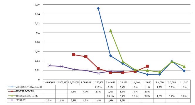
The International Conference on Smart and Innovative Agriculture                           IOP Publishing
IOP Conf. Series: Earth and Environmental Science 686 (2021) 012038    doi:10.1088/1755-1315/686/1/012038

3.3.Results of Sample Analysis of The Image-Scale Relationship
There were obtained a representative scale set to handle the different Google Earth images. These
scales were generated from the sample analysis, regarding the zoom functionality, within process
deepen - going back to each analyzed image resolution in various soil coverages (Table 3). The sample
analyzed varied in their lengths. The ranges have length dispersion as follows: 1) Agricultural land (93
– 665 m); 2) Infrastructure (178 – 1601 m; 3) Waterbodies (1417 – 21219 m); 4) Forest (14651 –
263999 m).
                Table 3. Representative Scales for Different Subjects from The Average
                                           Percentage Error
                           Agricultur       Water        Infrastructu
               Scale                                                           Forest
                                 al         bodies             re
           1:4,000,000                                                         3.0%
           1:2,000,000                                                         2.9%
           1:1,000,000                       5.3%                              2.2%
            1:500,000                        4.9%                              1.9%
            1:250,000         15.2%          2.4%                              1.4%
             1:66,000          5.1%          1.5%           10.5%              1.9%
             1:33,333          3.4%          1.6%            3.9%              1.8%
             1:16,666          1.9%          1.8%            2.1%
              1:8,000         1.1%           2.9%            2.0%
              1:4,000          1.2%                          1.6%
              1:2,000          3.9%                          3.9%
              1:1,000          1.9%                          2.8%
          (Source: Data Calculation, 2020)

   Regarding this variation, an average for each subject was defined to effectuate a statistical
sampling to verify their dispersion. In this case, for agricultural soil an average of 284 m was found;
water bodies with 6928.7 m; infrastructure with 475 m and forest 48320.9 m (Table 4). Likewise,
other statistical values were determined by the same lengths.
                          Table 4. Statistic Parameters of Sample Measurements
                               Agricultural   Water bodies        Infrastructure          Forest
            N                    32                 31                   32                28
       Average (m)             284.4              6928.7               475.0             48320.9
      Maximum (m)              665.0             21219.0               1601.0           263999.0
      Minimum (m)               93.0              1417.0               178.0             14651.0
        Variance             18057.9            18282865.7            122497.0        2334635704.3
   Standard deviation          134.4              4275.8               350.0             48318.1
   (Source: Data Calculation, 2020)

    To compare the sample lengths obtained by measuring on each scale with Jruler was estimated a
percentage error. This standardization was made to handle an error range, so that, for each sample, it
was obtained the difference based on calculated length measurement on the screen and the determined
measure with the Jruler, which describes the error. For example, to get the percentage error in
agricultural land subject to scale 1:250 000, a procedure was performed for each state of Mexico that
initially is calculated as follows: In agriculture case, it was obtained 375 m (long calculated) – 200 m
(measuring the sample length with Jruler) = 175 m of difference, then the 175 * 100/200 = 87.5%
error. The percentages for each sample taken at the same scale are summed and averaged, hence arose
the 15.2% for 1:250,000 scales in the agricultural land subject. Being given that was calculated the
same procedure for all 32 states, the result of each in other scales likewise is added and is determined

                                                     7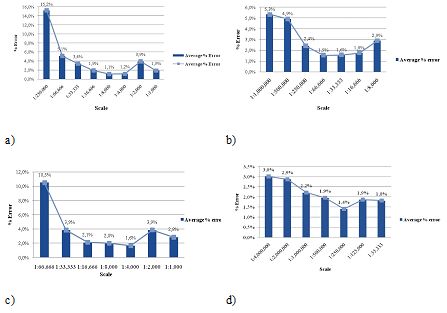
The International Conference on Smart and Innovative Agriculture                                IOP Publishing
IOP Conf. Series: Earth and Environmental Science 686 (2021) 012038         doi:10.1088/1755-1315/686/1/012038

average percentage error. Figure 5 shows the behavior from the average error percentage determined
in each sample analyzed of the four coverages. In these graphs describe similar patterns, showing that
the error is large in small scales, so that as scale increases until it exceeds half of the scale, it reaches
the smallest error, then, increased slightly.

  Figure 5. Average percentage error of samples of a) agricultural land, b) waterbody, c) infrastructure, and,
                                d) forest. (Source: Data Processing, 2020)

   By concentrating previous graphics into one shows the similarity between errors of four topics
discussed, which describes the following: By integrating scales to compare results in each of the
thematic percentages, shows that in the fifth level of each topic, the lowest value was found in the
error percentage, except water bodies, where the minimum is at the fourth scale (Figure 6).

  Figure 6. Comparative of average errors between agricultural land, water bodies, infrastructure, and forest
                                     (Source: Data Processing, 2020)

   In the first scale of each coverage (Agricultural land 1:250,000 - Waterbodies 1:1:000,000 -
Infrastructure 1:66,666 - Forest 1:4,000,000), the sample is perceived very small, from mm to a few
cm. In third and fourth scale (Agricultural land 1:33,333 and 1:16,666 - Waterbodies 1:250,000 and

                                                         8
The International Conference on Smart and Innovative Agriculture IOP Publishing
IOP Conf. Series: Earth and Environmental Science 686 (2021) 012038 doi:10.1088/1755-1315/686/1/012038
1:66,666 - Infrastructure 1:16,666 and 1:8000 - Forest 1:1,000,000 and 1:500,000), the sample is
observed moderate and can be measured on the screen. In the fifth scale (Agricultural land 1:8,000 -
Water Bodies 1:33,333 - Infrastructure 1:4,000 - Forest 1:250,000), the sample is fully viewed on the
screen, which facilitates direct measurement with the ruler. From the sixth scale (Agricultural land
1:4,000 - Waterbodies 1:16,666 - Infrastructure 1:2,000 - Forest 1:66,666), the sample exceeds the
screen, so must be measured several times with the ruler. Changes made to move the ruler, or the
sample causes the increase of the errors.
3.4 Variation of Error in Each Scale
In this case, both variables support to find a scale where there is greater variation among the errors,
that is, where the errors of the measurements are more likely to suffer more significant alterations.
Table 5 shows the variance and standard deviation obtained for each coverage. In this case, it can be
perceived as a similar pattern to the average error percentage.
Table 5. Variance and Standard Deviation for Damples of a) Agricultural Land, b) Waterbody, c) Infrastructure,
and, d) Forest
Figure 7 shows the graphics of the standard deviation. In these graphics is perceived that on a smaller
scale occurs more variation between the values calculated in samples. There is also a point after the
center where exists less dispersion, which shows after other increases.
Figure 7. Standard deviation for error percentage in a) agricultural, b) waterbodies, c) infrastructure, and,
d) forest.
9The International Conference on Smart and Innovative Agriculture IOP Publishing
IOP Conf. Series: Earth and Environmental Science 686 (2021) 012038 doi:10.1088/1755-1315/686/1/012038
Making a comparison between the results for the error percentage calculation and those results
determined based on the standard deviation calculation, are described in Table 6 and 7.
Table 6. Considering the Percentage Error Table 7. Considering the Percentage Error
Average Average
Land use Minimum Maximum Land use Minimum Maximum
error/Scale error/Scale error/Scale error/Scale
1.1% 15.2% 1.02% 18.69%
Agricultural Agricultural
(1:8,000) (1:250,000) (1:4,000) (1:250,000)
1.5% 5.3% 1.22% 7.02%
Water bodies Water bodies
(1:66,666) (1:1,000,000) (133.333) (1:500,000)
1.6% 10.5% 1.21% 18.39%
Infrastructure Infrastructure
(1:4,000) (1:66,666) (1:4,000) (1:66,666)
1.4% 3% 1.08% 2.46%
Forest Forest
(1:250,000) (1:4,000,000) (1:250,000) (1:2,000,000)
According to the Tabel 7, the obtained scales are recommended for associating the analyzed
coverages with Google Earth images. Such scales will allow getting a lower error and higher quality in
the various applications to be made with the image-scale relationship. The scales based on the average
of the error percentages determine the actual ranges between generated errors for each of the scales,
while scales determined based on the variation between errors, allow to find the scale where the error
percentage dispersion with respect its average is less. In the last decade, analyzes using tools such as
Google Earth have increased [25]. Accuracy is important in estimating natural resources and
infrastructure. For example, in China the Google Earth platform was used to calculate the extent of
bodies of water [26]; regarding infrastructure, terrain elevation data was obtained using Google Earth
to develop transportation applications [27]; furthermore, this platform was used to estimate changes in
land use [28], and, similarly, Google Earth is used to analyze the dynamics of agriculture [29]. High
precision was obtained in the four cases mentioned.
4. Conclusion
The present analysis confirmed the dependence between display scale and the associated error in the
interpretation of the soil coverages analyzed. As a result of this work, a catalogue of the scale-image
relationship was generated to facilitate the use of the Google Earth display system. This catalogue
affords to standardize the scale in Google Earth for certain purposes, besides defining the geographic
elements describing natural resources that can be used with a scale for endless studies and analyzes
carried out on the display system. The relation image-scale has been analyzed directly to associate the
real element represented in the images on a specific scale. The goal of this is to analyze the differences
between the measurement of vectorial data and their relationship with the images, since, according to
their resolution, inconsistencies are presented. As the scales increase, it is notable in any moment that
the observed object in the image is more significant and exceeds the screen size. This fact is due to the
zoom increment to adapt the view to the scale. It is worth mentioning that there are places on the
planet where the coverage of the image with good detail allows an increase in the image’s depth with
more zoom levels, of which there are more scales in those areas. Conversely, in other places with low
image resolution originate fewer zoom levels. Google Earth and other new technologies for spatial
data visualization and the applications developed of those systems, such that API's, development of
spatial data infrastructures and new research lines on Digital Earth, will have to answer in its time to
the quality representation needs of all geographic objects on the different territories.
10The International Conference on Smart and Innovative Agriculture IOP Publishing
IOP Conf. Series: Earth and Environmental Science 686 (2021) 012038 doi:10.1088/1755-1315/686/1/012038
References
[1] Chen, A., Leptoukh, G. G., Kempler, S. J., & Di, L. Visualization of Earth Science Data Using
Google Earth. The International Archives of the Photogrammetry, Remote Sensing and
Spatial Information Sciences. 34 (Part XXX), 6pp. (2010)
[2] Luque-Anaya, A. & Neves M., F. Digital territories: Google maps as a political technique in
the re-making of urban informality. Society and Space. 37 (3), pp. 449-467. doi:
10.1177/0263775818766069 . (2019).
[3] Mutanga, O. & Kumar, L. Google Earth Engine Applications. Remote Sensing. 11, 4pp. doi:
10.3390/rs11050591. (2019)
[4] Oxley, A. Web 2.0 applications of geographic and geospatial information. Bulletin of the
American Society for Information Science and Technology. 35 (4), pp. 43-48. doi:
10.1002/bult.2009.1720350412. (2009)
[5] Gorelick, N., Hancher, M., Dixon, M., Ilyushchenko, S., Thau, D. & Moore, R. Google Earth
Engine: Planetary-scale geospatial analysis for everyone. Remote Sensing of Environment.
202, pp. 18-27. doi: 10.1016/j.rse.2017.06.031 . (2017)
[6] Amani, M., Brisco, B., Afshar, M., Mirmazloumi, S. M., Mahdavi, S., Javad M., S. M., Huang,
W. & Granger, J. A generalized supervised classification scheme to produce provincial
wetland inventory maps: an application of Google Earth Engine for big geo data processing.
Big Earth Data. 3:4, pp. 378-394. doi: 10.1080/20964471.2019.1690404. (2019)
[7] Liang, J., Gong, J. & Li, W. Applications and impacts of Google Earth: A decadal review
(2006–2016). ISPRS Journal of Photogrammetry and Remote Sensing. 146, pp. 91-107. doi:
10.1016/j.isprsjprs.2018.08.019. (2018)
[8] Nativi, S. & Domenico, B. Enabling interoperability for Digital Earth: Earth Science coverage
access services. International Journal of Digital Earth. 2 (1), pp. 79-104. doi:
10.1080/17538940902866179. (2009)
[9] Sidhu, N., Pebesma, E. & Câmara, G. Using Google Earth Engine to detect land cover change:
Singapore as a use case. European Journal of Remote Sensing. 51 (1), pp. 486-500, doi:
10.1080/22797254.2018.1451782. (2018)
[10] Lefer, T. B., Anderson, M. R., Fornari, A., Lambert, A., Fletcher, J. & Baquero, M. Using
Google Earth as an Innovative Tool for Community Mapping. Public Health Reports. 123 (4):
pp. 474-480. doi: 10.1177/003335490812300408. (2008)
[11] Chen, J., Dowman, I., Li, S., Li, Z., Madden, M., Mills, J., Paparoditis, N., Rottensteiner, F.,
Sester, M., Toth, Ch., Trinder, J. & Heipke, C. Information from imagery: ISPRS scientific
vision and research agenda. ISPRS Journal of Photogrammetry and Remote Sensing. 115,
pp. 3-21. doi: 10.1016/j.isprsjprs.2015.09.008. (2016)
[12] Sajjad, A., Lu, J., Chen, X., Chisenga, Ch., Saleem, N. & Hassan, H. Operational Monitoring
and Damage Assessment of Riverine Flood-2014 in the Lower Chenab Plain, Punjab,
Pakistan, Using Remote Sensing and GIS Techniques. Remote Sensing. 12 (4), 26 pp. doi:
10.3390/rs12040714. (2020).
[13] Cárdenas T., A., Treviño G., E. J., Aguirre C., O. A., Jiménez P., J., González T., M. A. &
Antonio N., X. Spatial technologies to evaluate vectorial samples quality in maps production.
Investigaciones Geográficas, Boletín del Instituto de Geografía. 80, pp. 111-128. (2013).
[14] Porto de A., J., Herfort, B. & Eckle, M. The Tasks of the Crowd: A Typology of Tasks in
Geographic Information Crowdsourcing and a Case Study in Humanitarian Mapping.
Remote sensing. 8 (10), 22 pp. doi: 10.3390/rs8100859. (2016)
[15] Liu, D. & Kenjeres, S. Google-Earth Based Visualizations for Environmental Flows and
Pollutant Dispersion in Urban Areas. International Journal of Environmental Research and
Public Health. 14 (3), 16 pp. doi: 10.3390/ijerph14030247. (2017).
[16] Li, X., Ratti, C. & Seiferling, I.: ‘Mapping Urban Landscapes Along Streets Using Google
Street View’. ICACI 2017: Advances in Cartography and GIScience, Washington, USA,
May 2017, pp. 341 – 356. doi: /10.1007/978-3-319-57336-6_24
11The International Conference on Smart and Innovative Agriculture IOP Publishing
IOP Conf. Series: Earth and Environmental Science 686 (2021) 012038 doi:10.1088/1755-1315/686/1/012038
[17] Visser, V., Langdon, B., Pauchard, A. & Richardson, D. M. Unlocking the potential of Google
Earth as a tool in invasion science. Biological Invasions. 16, pp. 513–534. doi:
10.1007/s10530-013-0604-y. (2014)
[18] Ward, P.M. & Peters, P.A. Self-help housing and informal homesteading in peri-urban
America: Settlement identification using digital imagery and GIS. Habitat International. 31,
pp. 205-218. doi: 10.1016/j.habitatint.2007.02.001. (2007)
[19] Ziolkowska, J.R. & Reyes, R. Geological and hydrological visualization models for Digital
Earth representation. Computers & Geosciences. 94, pp. 31-39. doi:
10.1016/j.cageo.2016.06.003. (2016)
[20] Moorman, L. A. & Crichton, S. Learner Requirements and Geospatial Literacy Challenges for
Making Meaning with Google Earth. International Journal of Geospatial and Environmental
Research. 5 (3), 22 pp. (2018)
[21] Liu, G., He, J., Luo, K., Gao, P. & Ma, L. Scale-free networks of the earth's surface.
International Journal of Modern Physics B. 30 (21), 9pp. doi: 10.1142/S0217979216501435.
(2016).
[22] Gahlot, N., Dhara, M. & Prusty, G.: ‘Accuracy evaluation of various satellite imagery products
for large scale topographic mapping’. ISPRS TC V Mid-term Symposium “Geospatial
Technology – Pixel to People”, Dehradun, India, November 2018, pp. 105-110. doi:
10.5194/isprs-archives-XLII-5-105-2018
[23] El-Hallaq, M. A. & Hamad, M. I. Positional Accuracy of the Google Earth Imagery In The
Gaza Strip. Journal of Multidisciplinary Engineering Science and Technology. 4 (5), pp.
7249-7253. (2017)
[24] Tanner, C. C., & Cupertino, C. A. Asynchronous multilevel texture pipeline:
https://patents.google.com/patent/US6618053?oq=6618053. (2003).
[25] Yu, L. & Gong, P. Google Earth as a virtual globe tool for Earth science applications at the
global scale: progress and perspectives. International Journal of Remote Sensing. 33 (12),
pp. 3966-3986. DOI: 10.1080/01431161.2011.636081. (2012)
[26] Wang, Ch., Jia, M., Chen, N. & Wang. W. Long-Term Surface Water Dynamics Analysis Based
on Landsat Imagery and the Google Earth Engine Platform: A Case Study in the Middle
Yangtze River Basin. Remote Sensing. 10, 18pp. DOI: 10.3390/rs10101635. (2018).
[27] Wang, Y., Zou, Y., Henrickson, K., Wang, Y., Tang, J. & Park, B.-J. Google Earth elevation
data extraction and accuracy assessment for transportation applications. PLoS ONE. 12 (4),
17 pp. DOI: 10.1371/journal.pone.0175756. (2017)
[28] Venkatappa, M., Sasaki, N., Prasad S., R., Kumar T., N. & Ma, H.-O. Determination of
Vegetation Thresholds for Assessing Land Use and Land Use Changes in Cambodia using the
Google Earth Engine Cloud-Computing Platform. Remote sensing. 11 (13), 30 pp. DOI:
10.3390/rs11131514. (2019).
[29] Ou, C., Yang, J., Du, Z., Liu, Y., Feng, Q. & Zhu, D. Long-Term Mapping of a Greenhouse in a
Typical Protected Agricultural Region Using Landsat Imagery and the Google Earth Engine.
Remote Sensing. 12 (55): 23 pp. DOI: 10.3390/rs12010055. (2019)
12You can also read