Catchment tracers reveal discharge, recharge and sources of groundwater-borne pollutants in a novel lake modelling approach - Biogeosciences
←
→
Page content transcription
If your browser does not render page correctly, please read the page content below
Biogeosciences, 15, 1203–1216, 2018
https://doi.org/10.5194/bg-15-1203-2018
© Author(s) 2018. This work is distributed under
the Creative Commons Attribution 3.0 License.

Catchment tracers reveal discharge, recharge and sources of
groundwater-borne pollutants in a novel lake modelling approach
Emil Kristensen1 , Mikkel Madsen-Østerbye1 , Philippe Massicotte2 , Ole Pedersen1 , Stiig Markager2 , and
Theis Kragh1
1 The   Freshwater Biological Laboratory, Department of Biology, University of Copenhagen, Copenhagen, 2100, Denmark
2 Department   of Bioscience, Aarhus University, 4000, Roskilde, Denmark

Correspondence: Emil Kristensen (emil.kristensen@bio.ku.com)

Received: 23 May 2017 – Discussion started: 4 October 2017
Revised: 23 January 2018 – Accepted: 25 January 2018 – Published: 28 February 2018

Abstract. Groundwater-borne contaminants such as nutri-           2 years required a higher tracer concentration of inflowing
ents, dissolved organic carbon (DOC), coloured dissolved          water than found in any of the groundwater wells around the
organic matter (CDOM) and pesticides can have an impact           lake. From the estimations of inflowing tracer concentration,
the biological quality of lakes. The sources of pollutants can,   the CATS model isolated groundwater discharge sites located
however, be difficult to identify due to high heterogeneity in    mainly in the eastern part of the lake with a single site in the
groundwater flow patterns. This study presents a novel ap-        southern part. Observations from the eastern part of the lake
proach for fast hydrological surveys of small groundwater-        revealed an impermeable clay layer that promotes discharge
fed lakes using multiple groundwater-borne tracers. Water         during heavy precipitation events, which would otherwise be
samples were collected from the lake and temporary ground-        difficult to identify using traditional hydrological methods. In
water wells, installed every 50 m within a distance of 5–         comparison to the lake concentrations, high tracer concentra-
45 m to the shore, were analysed for tracer concentrations of     tions in the southern part showed that only a smaller fraction
CDOM, DOC, total dissolved nitrogen (TDN, groundwater             of water could originate from this area, thereby confirming
only), total nitrogen (TN, lake only), total dissolved phos-      the model results. A Euclidean cluster analysis of δ 18 O iso-
phorus (TDP, groundwater only), total phosphorus (TP, lake        topes identified recharge sites corresponding to areas adja-
only), δ 18 O / δ 16 O isotope ratios and fluorescent dissolved   cent to drainage channels, and a cluster analysis of the mi-
organic matter (FDOM) components derived from parallel            crobially influenced FDOM component C4 further identified
factor analysis (PARAFAC). The isolation of groundwater           five sites that showed a tendency towards high groundwater
recharge areas was based on δ 18 O measurements and areas         recharge rate. In conclusion, it was found that this method-
with a high groundwater recharge rate were identified using       ology can be applied to smaller lakes within a short time
a microbially influenced FDOM component. Groundwater              frame, providing useful information regarding the WRT of
discharge sites and the fractions of water delivered from the     the lake and more importantly the groundwater recharge and
individual sites were isolated with the Community Assembly        discharge sites around the lake. Thus, it is a tool for specific
via Trait Selection model (CATS). The CATS model utilized         management of the catchment.
tracer measurements of TDP, TDN, DOC and CDOM from
the groundwater samples and related these to the tracer mea-
surements of TN, TP, DOC and CDOM in the lake. A direct
comparison between the lake and the inflowing groundwater         1   Introduction
was possible as degradation rates of the tracers in the lake
were taken into account and related to a range of water reten-    Most lakes are connected to the groundwater, which to some
tion times (WRTs) of the lake (0.25–3.5 years in 0.25-year        degree defines their chemical and biological characteristics
increments). These estimations showed that WRTs above             (Lewandowski et al., 2015). Particularly in smaller lakes
                                                                  and ponds, the groundwater contributes nutrients, dissolved

Published by Copernicus Publications on behalf of the European Geosciences Union.
1204 E. Kristensen et al.: Catchment tracers reveal groundwater flow organic carbon (DOC), coloured dissolved organic matter hoft et al., 1990). The isotopic composition can also be re- (CDOM) or other contaminants, which can have a negative lated to evaporation lines (from the local evaporation line impact on the biological quality of the lakes (for nitrogen describing the δ 18 O and δ 2 H relationship) to estimate WRT and phosphorous, see review by Lewandowski et al., 2015). (Gibson et al., 2002). Overall, these tracers provide informa- These inputs often result in unfavourable light conditions tion on flow patterns in the terrain or WRT, but they do not for submerged macrophytes due to either increased phyto- provide information regarding discharge in specific areas or plankton biomass (Smith, 2003) or increased light absorption the concentrations of the previously mentioned pollutants in from high CDOM concentrations. The negative impacts of the discharging water. We propose a different approach uti- the contaminants make the identification of pollutant sources lizing both conservative and non-conservative tracers such as an important management issue for lakes, which, however, dissolved carbon and nutrients, which are partly transferred is complicated for groundwater due to temporal and spatial to the percolating groundwater on its way to the lake (Kid- differences in discharge and associated pollutant concentra- mose et al., 2011) and have a direct influence on the lake’s tions (e.g. Meinikmann et al., 2013). In addition, the lake biological structure. hydrology itself may be important, particularly in small wa- Some non-conservative tracers such as fluorescent dis- ter bodies. For example, low or fluctuating water level can solved organic matter (FDOM), which can be determined have a large influence on the biodiversity of the lake (Chow- using parallel factor analysis (PARAFAC), have been used Fraser et al., 1998). This illustrates the need for approaches to trace DOM in aquatic environments (He et al., 2014; Mas- to quickly identify discharge (i.e. groundwater exfiltrating sicotte and Frenette, 2011; Stedmon et al., 2003; Stedmon to the lake) and recharge (i.e. lake water infiltrating to the and Markager, 2005b; Walker et al., 2009). PARAFAC anal- groundwater) areas on the lake scale and thereby provide ysis is a modelling tool that can separate multiple FDOM the necessary tools for an effective management strategy for samples (emission and excitation matrices) into specific flu- ponds and small lakes. orescent components (Stedmon et al., 2003). The fluores- Groundwater discharge and recharge are traditionally cent components can be biologically produced proteins de- identified and quantified by measurements of the hydraulic rived from bacteria or molecules from the degradation of ter- head through the installation of piezometers around the lake restrial organic material. These components have previously and of the hydraulic conductivity in the sediments (Rosen- been found visually using a single excitation emission ma- berry et al., 2015). This method is often combined with the trix and the observed fluorescent peaks (Coble, 1996). The use of seepage meters, which quantify the water entering differentiation between the fluorescent components are both or leaving through the lake bottom (Lee and Cherry, 1979). a strength and a weakness as we can isolate many different However, this method is challenged by the heterogeneous components, but all of them can differ in both degradation nature of groundwater seepage related to the specific hy- and production rate in the lake and groundwater. Further- draulic conductivity of the lake bed sediments (Cherkauer more, these FDOM components have not yet been investi- and Nader, 1989; Kishel and Gerla, 2002; Rosenberry, 2005). gated as tracers in groundwater-fed lakes, as they, just as the Furthermore, these methods are also time-consuming as they rest of the non-conservative biological tracers, are volatile. have to be carried out several times throughout the sea- This is observed as a change in tracer concentrations (of- son. The heterogeneity and annual variability in groundwater ten a decrease) after the groundwater is discharged to the seepage call for a robust, easier and faster method to deter- lake. The speed at which the change in concentration occurs mine groundwater inputs and influences. is typically related to seasonal variations (e.g. temperature, Various conservative tracers have been used to achieve mixing of the water column and UV radiation) and the WRT estimates of groundwater flow and water retention times of the lake, e.g. the amount of time the tracer has been in the (WRTs) in lakes. These tracers are divided into three main lake. The removal and degradation rates have been examined categories: (1) environmental tracers (naturally derived trac- in many instances, e.g. for phosphorus (Larsen and Mercier, ers from the atmosphere or catchment that are transported 1976; Vollenweider, 1975), nitrate (Harrison et al., 2009; to the system), (2) historical tracers (anthropogenic tracers Jensen et al., 1995), CDOM and DOC (Madsen-Østerbye such as 3 H or 36 Cl from nuclear testing) or (3) applied trac- et al., 2018). In a modelling approach, these rates are impor- ers (tracers added to the system such as Br, Cl or fluorescent tant as they provide information about the change in tracer dyes) (Stets et al., 2010). Precipitation-derived environmen- concentration from the time when the tracer entered the lake. tal tracers, such as the isotope δ 18 O (reported in the Vienna- From this, it is possible to back-calculate the mixed inflow standard mean ocean water (SMOW), where δsample ‰ = concentration of specific tracers when they were discharged 1000((Rsample /Rsmow ) − 1) and R is the δ 18 O / δ 16 O ratio to the lake. These estimations are crucial when working with (Turner et al., 1987)), have been used to trace the interac- non-conservative tracers, as they enable a direct compari- tion between groundwater and surface water. As evapora- son between the tracer concentration found in the catchment tion occurs in the surface water it becomes enriched with and the estimated lake concentration before degradation took δ 18 O, producing a unique lake δ 18 O/δ 16 O ratio, which can place, which originates from the mixed inflow of groundwa- be traced in the areas with groundwater recharge (Krabben- ter. Biogeosciences, 15, 1203–1216, 2018 www.biogeosciences.net/15/1203/2018/
E. Kristensen et al.: Catchment tracers reveal groundwater flow                                                            1205

   As the concentrations of both conservative and non-            areas possess a high groundwater recharge rate and (3) if
conservative tracers in a groundwater-fed lake correspond to      catchment-derived tracer concentrations can be used to es-
the mixed concentrations of discharging groundwater, tak-         timate a range of WRTs, which can be used with the CATS
ing degradation and atmospheric deposition into account, it       model.
is possible to utilize the Community Assembly via Trait Se-
lection (CATS) approach. This model has been used to pre-
dict the relative abundances of a set of species from measures    2     Materials and methods
of community-aggregated trait values (average leaf area, root
length, etc.) for all plant species at a site (Shipley, 2009;     A small groundwater-fed lake in the sandy northwestern part
Shipley et al., 2006, 2011). The CATS model has three main        of Denmark was chosen for this study (Tvorup Hul, area:
parameters: (1) it models the probabilities that (2) maximize     4 ha, mean depth: 2.4 m, 56◦ 910 N, 8◦ 460 E, UTM Zone 32).
the entropy, which (3) is based on a set of constraints (Lalib-   Coniferous forest and heathland dominate the catchment, al-
erté et al., 2014; Shipley et al., 2011). In reality, the model   though some agricultural activities are found in the eastern
(1) predicts the relative abundances of species at a loca-        part of the catchment (Fig. 1a). Various isoetids including the
tion from their (3) average trait values by (2) minimizing        rare nationally threatened species Isoetes echinospora and
the number of species that explain the mean trait values.         Subularia aquatica inhabited the lake until some decades
Maximum entropy (2) is the maximizing of “new knowl-              ago when brownification increased significantly (based on
edge gained” related to plant communities. This means mov-        Rebsdorf, 1981, and the present study), probably due to in-
ing from “all species have the same relative abundances” to       creasing soil pH (Ekström et al., 2011). This led to a restora-
“a few species have a high relative abundance”. When ap-          tion attempt in 1992; a channel was established to bypass
plying the model to the lake–groundwater interaction, we          the stream going through the lake, thus making the lake fed
use the measured tracer concentrations at groundwater well        by groundwater. CDOM, DOC and the hydrologic conditions
sites around the lake as the individual plant species and the     in the lake have since been investigated in several projects
estimated mixed lake concentration before degradation took        (Madsen-Østerbye et al., 2018; Solvang, 2016). This has re-
place as the community-aggregated trait values.                   sulted in extensive background data as well as estimations
   Determining groundwater movement using both conserva-          of WRTs between 0.4 and 3.3 years based on water table
tive and non-conservative tracers found around the lake shore     heights, hydraulic conductivity and seepage meter samplings
overcomes some fundamental shortcomings related to tradi-         (Solvang, 2016, and preliminary work Peter Engesgaard, per-
tional sampling. Firstly, we often measure tracers, which do      sonal communications, 2017).
not have a direct impact on the lake ecosystem and there-
fore do not provide meaningful information regarding the          2.1    Sampling and laboratory analysis
inflow of nutrients or CDOM. Furthermore, the sampling is
only performed in a few places throughout the catchment,          A total of 30 groundwater samples were taken every 50 m
which does not necessarily provide all the information on the     around the lake within a distance of 5–45 m to the shore
groundwater flow patterns or to which degree water enters         in temporary groundwater wells at 1.25 m depth in Febru-
the lake and where. To overcome this, we measured conser-         ary 2016. The data preparation, analysis and results are vi-
vative and relevant non-conservative tracers in and around        sualized in Fig. 2. The water in the wells was replaced three
a small lake with the aim of developing a novel approach to       times before transferring the sample water to an acid-rinsed
identify groundwater discharge and recharge areas on a high       container. The samples were filtered through pre-combusted
spatial scale. Thus areas that deliver pollutants to the lake,    0.7 µm nominal pore size Whatman GF/F filters the same
in which groundwater recharge happens and where recharge          day and kept cool and dark in hermetically sealed acid-rinsed
occurs with an increased flow rate, were pinpointed. The lat-     BOD flasks until examination. Unfiltered samples were also
ter can spark further investigations into the lake WRT. In-       collected from the lake.
formation regarding the WRT of the lake is especially use-           DOC concentrations were measured using a total organic
ful when investigating how the concentrations of pollutants       carbon analyser (Shimadzu, Japan) in accordance with Kragh
in the lake will develop after future restoration attempts. In    and Søndergaard (2004). The CDOM absorbance was mea-
the present study, the eight following tracers were measured:     sured on a spectrophotometer (UV-1800, Shimadzu, Japan)
FDOM, CDOM, DOC, total dissolved phosphorus (TDP),                between 240 and 750 nm in 1 nm intervals in a 1 cm quartz
total dissolved nitrogen (TDN), total phosphorus (TP), to-        glass cuvette and expressed as the absorbance at 340 nm
tal nitrogen (TN) and δ 18 O / δ 16 O isotope ratios. For these   (ACDOM (340) cm−1 ). The samples were analysed for δ 18 O
tracers, we tested (1) if groundwater discharge sites and         and δ 16 O isotopes at the Department of Geosciences and
pollutant sources can be estimated with the CATS model            Natural Resource Management (University of Copenhagen)
based on tracer concentrations, (2) whether conservative and      using mass spectrometry in accordance with Appelo and
non-conservative tracers can be used to detect groundwa-          Postma (2005). δ 18 O is presented in the standard δ notation
ter recharge areas as well as provide insights into which         V-SMOW as δ 18 O ‰ (Vienna Standard Mean Ocean Water)

www.biogeosciences.net/15/1203/2018/                                                     Biogeosciences, 15, 1203–1216, 2018
1206                                                             E. Kristensen et al.: Catchment tracers reveal groundwater flow

Figure 1. (a) Aerial photo of Lake Tvorup Hul showing groundwater well sampling sites (numbers). Orange numbers denote groundwater
recharge sites, red numbers show sites with a high degree of recharge, white numbers represent possible groundwater discharge sites and light
blue shows model-isolated discharge sites. Positions a, b and c show the three sampling sites in the lake. Missing samples in the northeastern
part are due to an absence of groundwater in the area. The adjacent drainage channels north and west of the lake are marked with white lines.
(b) Inverse-distance-weighted (IDW) contour map of fluorescence component C4. The blue-green colour corresponds to lake concentrations;
darker blue indicates increased concentrations and lighter blue denotes decreased concentrations throughout the catchment. Areas with low
differences between fluorescence in the lake and in the catchment are seen north of the lake and indicate parts with a fast groundwater
recharge.

(Turner et al., 1987). TDP and TDN were determined for                   FDOM components. This allows for the detection of com-
groundwater samples while TN and TP were determined for                  ponents insufficiently represented in the collected samples
lake water, as inflowing nutrients become incorporated into              (Fellman et al., 2009; Stedmon and Bro, 2008; Stedmon and
aquatic organisms. Nutrients were measured by transferring               Markager, 2005a). The drEEM package was used to per-
5 mL sample water and 5 mL potassium persulfate reagent                  form the PARAFAC modelling following the same proce-
to acid-rinsed autoclave vials before autoclaving for 45 min.            dure as described in Murphy et al. (2013). A split-half anal-
Then 2.5 mL of borate buffer was added after cooling and                 ysis, in which the dataset is split into two parts and com-
analysed in an autoanalyser (AA3HRAutoAnalyzer, SEAL,                    pared multiple times, was used to test the results found in
USA) together with blanks and internal standard row.                     the PARAFAC model. A contour map showing the mea-
                                                                         sured FDOM concentrations in groundwater was plotted in
2.2    PARAFAC modelling                                                 ArcMap (ArcMap 10.4.1, ESRI, USA) using the inverse-
                                                                         distance-weighted (IDW) function with barriers fitted around
                                                                         the lake and drainage channels.
The fluorescent properties of DOM samples were investi-
gated using PARAFAC. The FDOM samples were initially
diluted 2–12 times to account for self-quenching, also re-               2.3    Groundwater recharge and areas with a high
ferred to as inner filter effect, which occurs with high CDOM                   groundwater recharge rate
absorbance in the sample (Kothawala et al., 2013). Sample
and blank fluorescence were measured using a spectrofluo-                A hierarchical Euclidean cluster of δ 18 O ‰ was employed
rometer (Cary Eclipse, Agilent Technologies, USA) by exci-               to determine groundwater recharge areas using the Stat base
tations between 240 and 450 nm, in 5 nm steps, while scan-               package in R. δ 18 O ‰ was chosen as it is both conser-
ning the emissions from 300 to 600 nm in 2 nm increments.                vative and biologically inert. Groundwater well sites that
Prior to PARAFAC analysis, fluorescence data were pro-                   formed a cluster together with the lake samples were con-
cessed in R (3.3.1) (R Core team, 2017) using the eemR                   sidered as being groundwater recharge sites, e.g. water orig-
(0.1.3) package. Blank values were subtracted following the              inating from the lake, and were excluded for the later es-
documentation provided in the eemR package to remove Ra-                 timations of groundwater discharge sites. The groundwater
man and Rayleigh scattering (Bahram et al., 2006; Lakow-                 recharge sites were further investigated using a range of non-
icz, 2006; Zepp et al., 2004). The data were then Raman                  conservative tracers influenced by biological degradation.
normalized by dividing the florescent intensities by the in-             We found that some of the tracer concentrations changed
tegral of the Raman peak of the blank sample (Lawaetz and                when moving from the lake to the groundwater. For exam-
Stedmon, 2009) and lastly corrected for the inner filter effect          ple, CDOM showed a decrease in concentration when enter-
(Kothawala et al., 2013) before being exported to MATLAB                 ing the groundwater, which is properly due to pH changes in
(2015b). In MATLAB, the fluorescence data were combined                  the soil. An inspection of the results revealed that a protein-
with a larger dataset (> 1000 fluorescent samples from Mas-              based fluorescent component met our criteria of being (1)
sicotte and Frenette (2011) originating from a range of di-              non-conservative, (2) not afflicted by the lake–groundwater
verse aquatic systems) in order to increase the diversity of             interface and (3) not too easily degraded or produced in

Biogeosciences, 15, 1203–1216, 2018                                                             www.biogeosciences.net/15/1203/2018/
E. Kristensen et al.: Catchment tracers reveal groundwater flow 1207
Collection of water samples Find appropriate degradation
from the lake and models for the desired tracers
groundwater wells close to related to the lake type and
the shore. The groundwater catchment area
samples are filtered
through a GF/F filter to
Data preparation
remove particles. From the lake concentrations
calculate the amount of
degraded tracer for a range of
WRTs to estimate the mixed
Determine the concentrations
concentration of tracers in the
of the chosen tracers in the
discharging groundwater.
samples
Relate these estimates with
measured groundwater
concentrations to find a
maximum WRT.
Choose a conservative tracer
and incorporate it into a
hierarchical Euclidean
dendrogram to isolate sites
that receive lake water Possible groundwater
discharge sites
are incorporated in the CATS
Split the dataset into model together with estimates
groundwater recharge sites of the mixed inflowing tracer
and possible groundwater concentration related to a
discharge sites range of possible WRTs
Analysis
Isolate one or more tracers
that are not afflicted in the
lake – groundwater interface The model isolates the least
while still being affected by number of sites that can
natural degradation over explain the measured tracer
time concentration in the lake and
the fraction of discharging
groundwater water each site
Incorporate the tracer/tracers is expected to deliver to the
into a hierarchical Euclidean lake
dendrogram to isolate sites
that resemble the lake and
indicate low retention time in
the soil, e.g. high recharge
rate
High flow-rate Groundwater Groundwater
recharge sites recharge sites discharge sites
Results
A cluster of the sites A cluster of the A combination of
that show a sites that sites that can
tendency towards resemble the lake explain the tracer
high groundwater concentration concentration in
discharge rate the lake
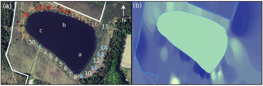
Figure 2. Diagram showing the workflow from data preparation to analysis to the results.
high amounts, which could create false positive groundwater 2.4 Non-conservative tracer degradation
recharge sites. The PARAFAC component was related to the and lake WRT
lake concentration with a hierarchical Euclidean cluster den-
drogram, and the sites that clustered together with the lake Lake WRT was found using traditional hydrological meth-
samples indicated a high groundwater recharge rate. ods combined with non-conservative tracer concentrations,
which were related to their degradation rates to form a proxy
www.biogeosciences.net/15/1203/2018/ Biogeosciences, 15, 1203–1216, 20181208 E. Kristensen et al.: Catchment tracers reveal groundwater flow
for the maximum WRT. Previous hydrological models sug- and degradation rates. Thus we were able to estimate the spe-
gested that the lake had a WRT between 0.4 and 3.3 years. To cific removal of DOC and CDOM on a monthly basis related
further narrow this range, we estimated WRT by relating the to the concentration measured in the lake at the time of sam-
concentrations found in the lake to their respective degrada- pling following Eq. (4):
tion rates related to increasing WRT, e.g. by adding the esti-
mated removed tracer since the groundwater entered the lake trlake = trlakepm − trlakepm · degra (frac) − trlakepm · mf
to the measured concentration in the lake. This enabled us + trinflow · mff, (4)
to narrow the span of the WRT based on the estimated mixed
inflowing tracer concentration related to the actual catchment where trlake is the lake concentration in the specific month,
concentrations. For example, if the estimated inflow concen- trlakepm is the lake tracer concentration in the previous month,
tration of a tracer is 100 µmol L−1 at a WRT of 2 years, and mff is the monthly flushing fraction (mff = 1/WRT/12), de-
the highest catchment tracer concentration is 50 µmol L−1 , gra (frac) is the degradation fraction in the present month re-
then the catchment does not support a WRT of 2 years. In lated to UV radiation and trinflow is the inflowing tracer con-
this instance, we estimated lake tracer concentrations of TN, centration. Equation (4) was solved for trinflow and calculated
TP, CDOM and DOC for WRTs from 0.25 to 3.5 years in using the same WRTs as the nitrate and phosphorus models.
0.25-year increments following Eq. (1):
2.5 The CATS model
trlake
MIC = , (1)
ret (frac) Since the concentrations of both conservative and non-
conservative tracers in a groundwater-fed lake correspond
where MIC is the mixed inflow concentration, trlake is the to the mixed concentrations of discharging groundwater,
tracer concentration found in the lake and ret (frac) is the while taking degradation and atmospheric deposition into
retention fraction of the tracer at a known WRT. Retention account, it is possible to utilize the CATS model. In the
models used in this study were based on the lake type as present study, the concentrations of non-conservative trac-
well as the geographical location of our lake. As there is not ers (DOC, CDOM, TDP and TDN) at groundwater well
one model that can provide removal rates across all lakes, sites around the lake acted as the individual plant species at
we encourage the readers to find models related to their spe- a site and the equilibrium tracer concentrations derived from
cific lake type. Thus, phosphorus equilibrium concentration Eq. (1) (DOC, CDOM, TP and TN) acted as the community-
in this study was found using Eq. (2) modified from Larsen aggregated trait values. When choosing tracers, it is impor-
and Mercier (1976), which describes phosphor retention in tant that there is differentiation between the concentrations
lakes with low productivity: measured at the sites. This means that a higher number of
1 tracers and higher uncorrelated concentration differences be-
retP (frac) = 1 − √ , (2) tween the sites result in a more secure determination of
1 + WRT
groundwater discharge sites. All tracers were investigated as
where retP (frac) is the retention fraction of phosphorus and a combined package, e.g. a single site is described by all the
WRT is the water retention time in the lake. Similarly, nitrate tracers mentioned above, and was run using the maxent func-
inflow concentrations were estimated using a modified Dan- tion in the FD (functional diversity) package in R to compute
ish nitrate removal model derived from Jensen et al. (1995) the CATS model (Laliberté et al., 2014). Further information
describing retention for shallow lakes with a short WRT (0– on the calculations can be found in the supplementary ma-
6 years) Eq. (3): terial for the FD package (Laliberté et al., 2014). From this,
the model predicts the minimum number of groundwater well
59 · WRT0.29 sites along the lake shore, which explains the measured con-
retN (frac) = , (3)
100 centrations in the recipient lake by maximizing the sites’ rel-
where retN (frac) is the retention fraction of nitrate and WRT ative contribution. The model also computes lambda values
is the water retention time in the lake. The corresponding from the least-squares regression measuring which tracers
retention fractions removed at different WRTs were related are most influential on the relative fractions of water originat-
to the lake concentrations to estimate what the mixed in- ing from the groundwater well sites. Consequently, lambda
flow concentration must have been to produce the present values quantify how much the relative contribution from the
lake concentration. The combined summer UV radiation and sites change when one tracer is changed a unit while the rest
bacterial degradation rates of DOC and CDOM in ground- of the tracers are kept constant.
water from the dominating catchment vegetation type of the
lake (Madsen-Østerbye et al., 2018) were extrapolated to the
rest of the year. This was performed by relating the degra-
dation rates to the mean monthly UV index (DMI, 2015)
while assuming a linear relationship between the UV index
Biogeosciences, 15, 1203–1216, 2018 www.biogeosciences.net/15/1203/2018/E. Kristensen et al.: Catchment tracers reveal groundwater flow 1209
Figure 3. Euclidean hierarchical clustering of the δ 18 O ‰ showing two clusters. The first cluster, marked with orange, groups with lake
samples and is therefore regarded as a recharge site. The other cluster, marked with light blue, is possible groundwater discharge sites to the
lake. The y axis denotes the linear distance between the δ 18 O ‰ samples fed to the model. The third lake sample was lost during preparation.
3 Results Stedmon et al. (2003) and is believed to be a combination
of fluorescent labile materials named peak N and T, which
3.1 Groundwater recharge are produced biologically associated with DOM degradation
(Coble, 1996; Stedmon and Markager, 2005b). Component
Recharge areas were identified with a Euclidean hierarchi- C5 is linked to free tryptophan, which is a product of micro-
cal cluster dendrogram of δ 18 O ‰. The cluster revealed two bial activity (Determann et al., 1998). This component has
main groups marked with orange and light blue in Fig. 3. The been found to decrease during dark incubations and UV ex-
first group (orange) shows the groundwater well sites, rang- posure (Stedmon et al., 2007), but component C5 is also as-
ing from sites 18 to 29, which clustered together with lake sociated with the degradation of DOM (Stedmon and Mark-
samples. The samples in this orange cluster share a clear re- ager, 2005b) and autochthonous production (Murphy et al.,
semblance with lake δ 18 O ‰ measurements and were there- 2008).
fore considered as groundwater recharge sites. The recharge The highest fluorescence concentrations were found in the
sites were located in the north and western part of the lake groundwater while the lake water fluorescence concentra-
and are marked with orange in Fig. 1a. tions were generally lower (Table S1). Component C1 had
the highest fluorescence with a value of 7.8 Raman’s units
3.2 Fluorescent DOM (R.U.) in the lake and a maximum fluorescence of 47.1 R.U.
at groundwater well site 7. Component C5 had the lowest
PARAFAC and split-half analysis modelling identified five fluorescence in the lake (0.27 R.U.) and a maximum fluores-
distinct fluorescent DOM components (C1–C5, explained cence of 2.9 R.U. at groundwater well site number 8. Com-
variance 96.79 %). The spectral properties of the five fluo- ponent C5 also varied much between groundwater samples
rophores (components) identified by the PARAFAC analy- with the lowest value of 0.1 R.U. or 28 times lower than the
sis (Fig. 4) revealed that the DOM pool had both terrestrial maximum concentration. Components C1, C2 and C3 had
and microbial influence. Component C1 was similar to previ- low lake-like concentrations in recharge areas (orange sites
ously found components from terrestrial humic-like material in Fig. 1a). Concentrations of C4 were generally higher in
(Stedmon et al., 2003). The component absorbs in the UV-C groundwater around the lake than in the lake (1.1–1.5 vs.
region, which is absorbed by the ozone layer and atmosphere 1.1 R.U. visualized in Fig. 1b). Component C4 was chosen
(Diffey, 2002), and is for this reason expected to be mainly as a proxy for groundwater recharge as the concentration
photo-resistant (Ishii and Boyer, 2012). Component C2 has of the C4 component increase with biological activity and
been reported to be both marine and terrestrial humic-like there were no apparent concentration changes in the lake–
(Coble, 1996; Murphy et al., 2006) and seems to be degraded groundwater interface. The cluster diagram of component C4
by visible light and produced by microbial degradation in showed that especially site 24 grouped with lake samples, but
equal amounts (Stedmon and Markager, 2005b). Component sites 20, 21, 23 and 26 also showed high comparability with
C3 was also believed to be of terrestrial humic-like origin the lake (Fig. 5), which can also be observed from the IDW
and was similar to the fluorescent peak C described by Coble map of component C4 around the lake (Fig. 1b).
(1996). The component absorbs in the UV-A region and is
susceptible to both microbial and photochemical degradation 3.3 Groundwater discharge areas and lake WRT
(Stedmon et al., 2007; Stedmon and Markager, 2005a). Com-
ponent C3 may be an intermediate product or produced bio- Tracer concentrations of the lake narrowed down the possible
logically since changes in the concentration have been ob- WRT. Equilibrium tracer concentrations of DOC, CDOM,
served in the open oceans and in sea ice that has no apparent TDP and TDN (found using Eqs. 1–4) for WRTs between
connection to the terrestrial environment (Ishii and Boyer, 0.25 and 3.5 years in 0.25-year increments revealed that con-
2012). Component C4 is similar to component 5 found in centrations of TDN in the catchment are not high enough
www.biogeosciences.net/15/1203/2018/ Biogeosciences, 15, 1203–1216, 20181210 E. Kristensen et al.: Catchment tracers reveal groundwater flow
550 20 % for ACDOM (340) in the same months and were sig-
C1
500 nificantly different from each other (P < 0.001). Thus, esti-
Em. (nm) 450
mated mixed inflow concentrations of CDOM ranged from
ACDOM (340) = 0.43 to 1.04 cm−1 while DOC ranged from
400
1205 to 3160 µmol L−1 for a WRT between 0.25 and 2 years
350
(Eqs. 1 and 4). The CATS model isolated the minimum num-
300 Comp 1 ber of sites that explained the estimated lake concentrations.
C2 The model identified sites 1, 9, 11, 13 and 14 as the ground-
500
water discharge sites delivering more than 0.1 % of the water
450 throughout the different WRTs (Fig. 6). Changes in site dis-
Em. (nm)
400 tribution and fractions of discharging water were observed
350
between the different WRTs, but in general, groundwater
Comp 2
from 3–4 sites explains the estimated concentrations in the
300
lake (Fig. 6). Site number 14 delivers more water with a
C3
500
higher WRT (to a maximum of 54 % of the total discharge).
Site 1 peaks at a WRT of 1.25, providing 27 % of the water
450
Em. (nm)
to the lake. Site number 9 delivers less water with increasing
400 WRT, but 49 % at the lowest WRT of 0.25 years. Site number
350 11 delivers 26 to 34 % of the water to the lake until a WRT
300 Comp 3 above 1.5 years is reached, at which site 13 explains the con-
C4 centration in the lake better and provides 29 and 19 % of the
500 water to the lake. Overall, 73 to 96 % of the water is esti-
450
mated to arrive from the eastern part of the lake, while site
Em. (nm)
number 1 (in the southern part) is estimated to deliver 4 to
400
27 % of the water. Lambda values, explaining which tracers
350
are the most important when predicting the fractions of water
Comp 4
300 originating from groundwater well sites, showed that CDOM
C5 was the most important tracer when determining which sites
500
delivered water to the lake with a mean lambda value for all
450 WRTs of 24.2 vs. 0.1–5.9 for the other tracers.
Em. (nm)
400
350
4 Discussion
300 Comp 5
250 300 350 400 450 The combination of biological and hydrological methods in
Ex. (nm)
a novel approach provided a better estimate of the WRT,
Figure 4. Spectral properties of the five PARAFAC components an identification of groundwater recharge and discharge ar-
(C1–C5) found in this study. The x axis shows the excitation (Ex) eas, and the fractions of water coming from each site. Based
wavelength in nanometres (nm) and the y axis shows the emission on the model results and earlier hydrological studies, we
(Em) wavelength in nanometres (nm) with low fluorescence being will discuss the main questions from the introduction (1) if
blue and high being red. groundwater discharge sites and pollutant sources can be es-
timated with the CATS model based on tracer concentrations,
(2) whether conservative and non-conservative tracers can be
used to detect groundwater recharge areas as well as provide
to support WRT values over 2 years based on the nitrogen
insights into which areas have a high groundwater recharge
retention model used. Thus, catchment tracer data revealed
rate and (3) if catchment-derived tracer concentrations can
a possible WRT between 0 and 2 years.
be used to estimate a range of the WRTs, which can be used
Groundwater discharge areas were found employing the
with the CATS model. Furthermore, we will discuss which
CATS model on nutrient concentrations and DOM fractions
of the tracers work and which could possibly work with re-
estimated using Eq. (1). related to WRTs between 0.25 and
fined methods, as well as how these findings could benefit
2 years. The estimated phosphorus concentrations ranged
lake restoration programmes.
from 46 to 80 µg PL−1 (Eqs. 1 and 2) while nitrate con-
centrations ranged from 1113 to 2417 µg NL−1 (Eqs. 1
and 3). CDOM and DOC degradation rates were related
to the UV index and varied from 0.64 % in December to
28 % per month in June for DOC and between 0.46 and
Biogeosciences, 15, 1203–1216, 2018 www.biogeosciences.net/15/1203/2018/E. Kristensen et al.: Catchment tracers reveal groundwater flow 1211
Figure 5. Euclidean hierarchical clustering of fluorescent component C4 from recharging groundwater sites. The fluorescence found at sites
20, 21, 23, 24 and 26 clusters together with lake fluorescence (marked red). This indicates that these sites have a high degree of groundwater
recharge. Groundwater well site 24 seems to be especially important in this regard.
1 9 11 13 14
0.5
0.4
Fraction
0.3
0.2
0.1
0.0
0.25
0.5
0.75
1
1.25
1.5
1.75
2
0.25
0.5
0.75
1
1.25
1.5
1.75
2
0.25
0.5
0.75
1
1.25
1.5
1.75
2
0.25
0.5
0.75
1
1.25
1.5
1.75
2
0.25
0.5
0.75
1
1.25
1.5
1.75
2
Water retention time
Figure 6. Results derived from the CATS model shown in a bar plot in which the groundwater well sites (their numbering) are seen on the
top x axis and the fractions of groundwater discharge estimated to derive from the sites are shown on the y axis (only the sites that deliver
more than 0.1 % water to the lake are shown). The bottom x axis denotes the different water retention times used in this model. Three to four
sites generally explain the estimated concentrations in the lake.
4.1 Determination of groundwater recharge areas lake formed a group (sites 24, 20, 21, 23 and 26) (Fig. 5 and
visually in Fig. 1b). This information can be of importance
related to placement of seepage meters, which will result in
Groundwater recharge sites were identified along the north- better estimations of the groundwater discharge and recharge
ern and western part of Tvorup Hul with a hierarchical and as such the modelled WRT of the lake. In other words, it
cluster analysis of the conservative δ 18 O tracer. The exact might be advantageous to carry out groundwater sampling
same areas are also the ones with adjacent drainage channels first to estimate sites with high discharge rates, then esti-
(Fig. 1a), which facilitate the areas as recharge sites. While mate WRT, utilizing these sites and finally model ground-
δ 18 O ‰ worked well as a general groundwater recharge es- water discharge areas by using the improved and narrowed
timator, it does not indicate which sites deliver more water. WRT range.
An indication of this can be found when examining the non- CDOM generally showed much lower absorbance at
conservative tracers such as the fluorescent components. groundwater recharge sites than in the lake, making it less
Sites resembling the fluorescence found in the lake will suitable for estimating recharge areas. The decrease in ab-
indicate a high groundwater recharge rate, while a differ- sorption is possibly due to low soil pH, causing flocculation
ence in concentration between lake and groundwater sites of CDOM in the soil matrix (Ekström et al., 2011). The same
will indicate a lower groundwater recharge rate where there was observed with fluorescence of component C1, which had
is sufficient time for a significant modification of the com- lower intensities in recharge areas, indicating that component
ponents representing the DOM pool of the lake. The fluo- C1 is linked to CDOM. While component C1 was not partic-
rescent component C4 has previously been found to increase ularly useful for estimating groundwater recharge, it could be
with biological activity (Coble, 1996), which is why we used useful to estimate discharge sites. To utilize the component
it as a proxy to estimate the sites with a high groundwater for discharge estimates there is a need for an assessment of
recharge rate. The hierarchical Euclidean cluster dendrogram the degradation rate. While it has been shown that component
of component C4 showed that sites in the northern part of the
www.biogeosciences.net/15/1203/2018/ Biogeosciences, 15, 1203–1216, 20181212 E. Kristensen et al.: Catchment tracers reveal groundwater flow
C1 is largely photo-resistant, as it does not absorb the UV- multi-tracer approach enables the determination of discharge
A radiation areas and is largely resistant to microbial degra- areas much more precisely and on a temporal scale related
dation processes (Ishii and Boyer, 2012), no reliable rates to the WRT of the lake (in this instance the previous 3 to
for the degradation have been found. In this study, we found 24 months). Consequently, the model is able to track uncom-
that only sites number 9 and number 11 hold concentrations mon events such as heavy precipitation events in which a
lower than the lake (Table S1), indicating that most ground- large amount of water is discharged to the lake during a short
water discharge would originate from these sites if little to no period. These events are often difficult to track as seepage
degradation takes place. meters need to be deployed in this exact period as well as in
the right places.
4.2 Determination of groundwater discharge areas
4.3 Tracer influences
Neither δ 18 O nor previous seepage meter samplings have
achieved a similar understanding of groundwater recharge Most tracers used in this study are less conservative com-
areas in Tvorup Hul as compared to the present approach. pared to δ 18 O and can therefore change both in the lake wa-
While the δ 18 O ‰ provides a way of separating ground- ter and in the catchment soils. This entails an understanding
water and surface water, using it to determine groundwa- of processes and rates that influence the concentrations. The
ter discharge sites is simply not possible due to the homo- temporal variability in nitrate concentrations in groundwa-
logical distribution seen in groundwater (Krabbenhoft et al., ter are related to the flow rate rather than seasonal changes
1990). Previous seepage meter samplings provided scattered (Kennedy et al., 2009). The same was observed for phos-
and momentary estimations of discharge sites, indicating phorus, where particularly dry periods followed by heavy
that groundwater entered the lake from the southern bank rain increased the phosphorus concentration measured in
(Solvang, 2016). This does not correspond to tracer con- groundwater-fed springs (Kilroy and Coxon, 2005). Thus,
centrations found in the southern area, which show very in the case of northern Europe, sampling during late win-
high CDOM absorbance at 340 nm (ACDOM (340) = 1.3– ter might be the best solution because soils are saturated at
3.1 cm−1 ) and DOC concentrations (3114–10 467 µmol L−1 ) this time of year (Sand-Jensen and Lindegaard, 2004). Previ-
in relation to the lake (ACDOM (340) = 0.4 cm−1 /DOC ously polluted areas, e.g. from wastewater infiltration, with
1058 µmol L−1 ). This hints that the lake is influenced by increased concentrations of DOC and nutrients are likely
groundwater discharge from other areas as well. The lowest to be in a state of imbalance, resulting in a reduction in
DOC concentrations in the southern area were several times concentrations over time (Repert et al., 2006). For this rea-
higher than those from the equilibrium estimation, suggest- son, in these areas, it is important to conduct temporal sam-
ing a WRT above 6 years, which is well beyond previous pling following decreases in concentrations and to relate the
estimates of WRT. Samples from the eastern shore had lower samples to lake concentrations during sampling. Lake inter-
concentrations all around, proposing that water from this area annual DOC and CDOM changes were generally low in our
influences the lake water. Thus, if the water actually origi- study with an annual ACDOM (340) = 0.41 cm−1 ± SD 0.05,
nated from the southern area, the lake would need to have corresponding to what is observed in larger water bodies
a prolonged WRT, resulting in increased removal of tracers where WRT integrates inflowing DOC and CDOM (Winter-
from the lake. This requirement conflicts with the remain- dahl et al., 2014). Inter-annual DOC and CDOM variations
ing tracers, for which especially TDN sets an upper limit of in groundwater from the lake catchment (Fig. S1) showed the
2 years to the WRT. same tendency as described for nutrients, and this suggests
The CATS model used in this study shows that while that sampling should be performed at multiple times or in
a fraction of groundwater enters the lake from the southern a period without drought or high rainfall. On a broader scale,
bank, most of the water originates from the eastern shore the variation in DOC is known to be related to hydrology
(Fig. 1a). Seepage meter measurements from the eastern (Erlandsson et al., 2008), mean air temperature (Winterdahl
shore showed both discharging and recharging of ground- et al., 2014) and the recovery from acid deposition (Evans
water (Solvang, 2016). The same was observed for δ 18 O ‰ et al., 2006; Monteith et al., 2007). Sampling from wet areas
samples from the eastern part of the lake, which were lower with standing surface water resulted in high concentrations
than in the groundwater from the southern shore, indicating of most tracers (Table S1). Consequently, these areas should
an influence of newly precipitated water or influence from be avoided, seeing that they provide no information regard-
the lake. Sampling in the northeastern and eastern part of the ing the discharge of groundwater. The removal of CDOM and
lake revealed an area with little groundwater and a clay de- DOC also changes on an annual basis in lakes and is related
posit layer that possibly reduces infiltration to deeper ground- to bacterial degradation, photodegradation, sources and mix-
water layers. As a result, precipitations could enter the lake ing of the water column. A sensitivity analysis of the results
as surface and subsurface run-off water originating from the was conducted by running the CATS model with a ±10 %
hills to the east and the plateau in the northeastern corner change in tracer concentrations. The results showed that sites
(Fig. 1a), resulting in short bursts of discharging water. The generally remained unchanged with only smaller deviations
Biogeosciences, 15, 1203–1216, 2018 www.biogeosciences.net/15/1203/2018/E. Kristensen et al.: Catchment tracers reveal groundwater flow 1213
in percent-wise distribution in discharge up to a WRT of in lakes with short WRT (Weyhenmeyer et al., 2016). This
1.25 years (Fig. S2). Above this point, there are some dif- makes it critical to establish a modelling tool that is capable
ferences in sites, which change between sites number 11 of pinpointing sites delivering pollutants to lakes and provide
and number 13. In conclusion, even when changing multi- us with the ability to take action and reduce the impact on the
ple parameters in the model, the same five groundwater wells ecological state of lakes.
are identified, explaining the measured lake concentrations.
Future investigations into variation in tracers in groundwa-
ter and degradation rates in lakes will likely strengthen this 5 Conclusions
model.
The processes that influence changes in FDOM are still be- The present method and modelling tool can improve esti-
ing investigated (Ishii and Boyer, 2012). Tracing FDOM has mates of recharge and discharge areas as well as WRT in
been conducted in both rivers and open waters (Baker, 2001, smaller lakes on a temporal scale. The model provides ac-
2002; Stedmon and Markager, 2005a), but only a few stud- curate estimates of discharge fractions, related to field mea-
ies have been conducted in groundwater. These studies have surements, and can be used for precise management of prob-
focused on changes in FDOM from deep groundwater wells lematic pollution areas. The hierarchical clustering can be
(Lapworth et al., 2008) or tracing FDOM using samples that used to estimate groundwater recharge sites, which can be
are collected very far apart (Chen et al., 2010). Specific fluo- incorporated as a guideline for a better estimation of WRT
rescence intensity of components showed large differences in lakes. Furthermore, the use of multiple tracers strengthens
among sites in this study, up to a factor of 28, between the model and keeps a certain degree of freedom in regard to
groundwater well sites, with the lowest at site 11 and high- the choice of tracers related to laboratory capabilities.
est at site 8, around the relatively small lake. These findings
illustrate the problem when applying FDOM as a tracer over
large distances in groundwater. In addition to bio- and pho- Data availability. The underlying data can be accessed in the Sup-
plement (Table S1).
todegradation of fluorescent components, absorption changes
have also been observed in relation to Fe(III) concentrations
(Klapper et al., 2002). This might change the concentrations
of FDOM components as they travel from anoxic ground- The Supplement related to this article is available online
water with reduced iron into the oxic lake water. Overall, at https://doi.org/10.5194/bg-15-1203-2018-supplement.
PARAFAC components have the potential to work as ground-
water tracers, but there is a need for a better understanding
of the processes that cause changes in fluorescence character-
istics of DOM and hence concentrations of FDOM compo-
nents both in the lake and in the lake–groundwater interface. Competing interests. The authors declare that they have no conflict
of interest.
4.4 Potential lake management influence
Acknowledgements. We are grateful to Naturstyrelsen (the Depart-
The determination of discharge sites can result in direct man-
ment for Nature and Conservation) for access to the study area
agement related to specific problematic areas. The model in Nationalpark Thy. The study was partly supported by a grant
used in this study showed that water entering the lake pri- to the Centre for Lake Restoration, a Villum Kann Rasmussen
marily originated from the catchment to the east of the Centre of Excellence. Peter Engesgaard and Ingeborg Solvang are
lake. If water from this part were diverted around the lake, acknowledged for their comments on the paper and for supplying
there would be a reduction in CDOM absorbance of 61– data on oxygen isotopes.
89 % based on calculations relating percent-wise discharge,
its concentrations and WRTs from 0.25 to 2 years in 0.25- Edited by: Florian Wittmann
year increments. Conversely, diverting water around the lake Reviewed by: two anonymous referees
at site number 1 would only result in a lowered inflowing
CDOM absorbance of 11–39 %. Moreover, in both cases,
there would be an increase in photobleaching of present
CDOM in the lake caused by the increased WRT. Further- References
more, huge reductions would occur for TP and TN, with a de-
Appelo, C. A. and Postma, D.: Geochemistry, Groundwater and Pol-
crease of 82–96 % if diverting water from the eastern shore, lution, Balkema, 2005.
in contrast to the southern shore with a modelled decrease of Bahram, M., Bro, R., Stedmon, C., and Afkhami, A.: Handling of
4–18 % in TP and TN. In the future, hydrology is likely to Rayleigh and Raman scatter for PARAFAC modeling of fluo-
be the main driver of variability in DOM (Erlandsson et al., rescence data using interpolation, J. Chemometr., 20, 99–105,
2008) with an estimated increase in CDOM by a factor of 4 https://doi.org/10.1002/cem.978, 2006.
www.biogeosciences.net/15/1203/2018/ Biogeosciences, 15, 1203–1216, 20181214 E. Kristensen et al.: Catchment tracers reveal groundwater flow Baker, A.: Fluorescence excitation - Emission matrix characteriza- ment runoff using stable isotopes: modelling and results from tion of some sewage-impacted rivers, Environ. Sci. Technol., 35, a regional survey of Boreal lakes, J. Hydrol., 262, 128–144, 948–953, https://doi.org/10.1021/es000177t, 2001. https://doi.org/10.1016/S0022-1694(02)00022-7, 2002. Baker, A.: Spectrophotometric discrimination of river dis- Harrison, J. A., Maranger, R. J., Alexander, R. B., Giblin, A. E., solved organic matter, Hydrol. Process., 16, 3203–3213, Jacinthe, P. A., Mayorga, E., Seitzinger, S. P., Sobota, D. J., and https://doi.org/10.1002/hyp.1097, 2002. Wollheim, W. M.: The regional and global significance of nitro- Chen, M., Price, R. M., Yamashita, Y., and Jaffé, R.: Com- gen removal in lakes and reservoirs, Biogeochemistry, 93, 143– parative study of dissolved organic matter from ground- 157, https://doi.org/10.1007/s10533-008-9272-x, 2009. water and surface water in the Florida coastal Ever- He, X. S., Xi, B. D., Gao, R. T., Wang, L., Ma, Y., Cui, D. Y., glades using multi-dimensional spectrofluorometry combined and Tan, W. B.: Using fluorescence spectroscopy coupled with multivariate statistics, Appl. Geochem., 25, 872–880, with chemometric analysis to investigate the origin, compo- https://doi.org/10.1016/j.apgeochem.2010.03.005, 2010. sition, and dynamics of dissolved organic matter in leachate- Cherkauer, D. S. and Nader, D. C.: Distribution of ground- polluted groundwater, Environ. Sci. Pollut. R., 22, 8499–8506, water seepage to large surface-water bodies: the effect https://doi.org/10.1007/s11356-014-4029-7, 2014. of hydraulic heterogeneities, J. Hydrol., 109, 151–165, Ishii, S. K. L. and Boyer, T. H.: Behavior of reoccurring parafac https://doi.org/10.1016/0022-1694(89)90012-7, 1989. components in fluorescent dissolved organic matter in natural Chow-Fraser, P., Lougheed, V., Le Thiec, V., Crosbie, B., and engineered systems: a critical review, Environ. Sci. Technol., Simser, L., and Lord, J.: Long-term response of the biotic 46, 2006–2017, https://doi.org/10.1021/es2043504, 2012. community to fluctuating water levels and changes in wa- Jensen, J. P., Lauridsen, T. L., Søndergaard, M., Jeppesen, E., ter quality in Cootes Paradise Marsh, a degraded coastal Agerbo, E., and Sortkjær, L.: Ferske Vandområder – Søer, Vand- wetland of Lake Ontario, Wetl. Ecol. Manag., 6, 19–42, miljøplanens overvågningsprogram 1995, 96, 1995. https://doi.org/10.1023/A:1008491520668, 1998. Kennedy, C. D., Genereux, D. P., Corbett, D. R., and Mi- Coble, P. G.: Characterization of marine and terrestrial DOM tasova, H.: Spatial and temporal dynamics of coupled in seawater using excitation-emission matrix spectroscopy, groundwater and nitrogen fluxes through a streambed in Mar. Chem., 51, 325–346, https://doi.org/10.1016/0304- an agricultural watershed, Water Resour. Res., 45, W09401, 4203(95)00062-3, 1996. https://doi.org/10.1029/2008WR007397, 2009. Determann, S., Lobbes, J. M., Reuter, R., and Rullkötter, J.: Kidmose, J., Engesgaard, P., Nilsson, B., Laier, T., and Ultraviolet fluorescence excitation and emission spectroscopy Looms, M. C.: Spatial distribution of seepage at a flow-through of marine algae and bacteria, Mar. Chem., 62, 137–156, lake: Lake Hampen, Western Denmark, Vadose Zone J., 10, 110– https://doi.org/10.1016/S0304-4203(98)00026-7, 1998. 124, https://doi.org/10.2136/vzj2010.0017, 2011. Diffey, B. L.: Sources and measurement of ultraviolet ra- Kilroy, G. and Coxon, C.: Temporal variability of phosphorus diation, Methods, 28, 4–13, https://doi.org/10.1016/S1046- fractions in Irish karst springs, Environ. Geol., 47, 421–430, 2023(02)00204-9, 2002. https://doi.org/10.1007/s00254-004-1171-4, 2005. DMI: UV-dose: DMI, available at: http://www.dmi.dk/vejr/ Kishel, H. F. and Gerla, P. J.: Characteristics of preferential flow and sundhedsvejr/uv-indeks/uv-dose/ (last access: 12 May 2016), groundwater discharge to Shingobee Lake, Minnesota, USA, Hy- 2015. drol. Process., 16, 1921–1934, https://doi.org/10.1002/hyp.363, Ekström, S. M., Kritzberg, E. S., Kleja, D. B., Larsson, N., 2002. Nilsson, P. A., Graneli, W., and Bergkvist, B.: Effect of Klapper, L., McKnight, D. M., Fulton, J. R., Blunt-Harris, E. L., acid deposition on quantity and quality of dissolved organic Nevin, K. P., Lovley, D. R., and Hatcher, P. G.: Ful- matter in soil water, Environ. Sci. Technol., 45, 4733–4739, vic acid oxidation state detection using fluorescence https://doi.org/10.1021/es104126f, 2011. spectroscopy, Environ. Sci. Technol., 36, 3170–3175, Erlandsson, M., Buffam, I., Fölster, J., Laudon, H., Temnerud, J., https://doi.org/10.1021/es0109702, 2002. Weyhenmeyer, G. A., and Bishop, K.: Thirty-five years of Kothawala, D. N., Murphy, K. R., Stedmon, C. A., Weyhen- synchrony in the organic matter concentrations of Swedish meyer, G. A., and Tranvik, L. J.: Inner filter correction of dis- rivers explained by variation in flow and sulphate, Glob. solved organic matter fluorescence, Limnol. Oceanogr.-Meth., Change Biol., 14, 1191–1198, https://doi.org/10.1111/j.1365- 11, 616–630, https://doi.org/10.4319/lom.2013.11.616, 2013. 2486.2008.01551.x, 2008. Krabbenhoft, D. P., Bowser, C. J., Anderson, M. P., and Val- Evans, C. D., Chapman, P. J., Clark, J. M., Monteith, D. T., and ley, J. W.: Estimating groundwater exchange with lakes: 1. The Cresser, M. S.: Alternative explanations for rising dissolved or- stable isotope mass balance method, Water Resour. Res., 26, ganic carbon export from organic soils, Glob. Change Biol., 12, 2445–2453, https://doi.org/10.1029/WR026i010p02445, 1990. 2044–2053, https://doi.org/10.1111/j.1365-2486.2006.01241.x, Kragh, T. and Søndergaard, M.: Production and bioavailabil- 2006. ity of autochthonous dissolved organic carbon: effects Fellman, J. B., Miller, M. P., Cory, R. M., D’Amore, D. V., of mesozooplankton, Aquat. Microb. Ecol., 36, 61–72, and White, D.: Characterizing dissolved organic matter using https://doi.org/10.3354/ame036061, 2004. PARAFAC modeling of fluorescence spectroscopy: a compar- Lakowicz, J. R.: Principles of Fluorescence Spectroscopy, edited ison of two models, Environ. Sci. Technol., 43, 6228–6234, by: Lakowicz, J. R., Springer US, Boston, MA, 2006. https://doi.org/10.1021/es900143g, 2009. Laliberté, E., Legendre, P., and Shipley, B.: Measuring func- Gibson, J. J., Prepas, E. E., and McEachern, P.: Quantita- tional diversity from multiple traits, and other tools for func- tive comparison of lake throughflow, residency, and catch- tional ecology, available at: http://citeseerx.ist.psu.edu/viewdoc/ Biogeosciences, 15, 1203–1216, 2018 www.biogeosciences.net/15/1203/2018/
You can also read