CERES Satellite and Climate Sensitivity

CERES Satellite and Climate Sensitivity
by Ken Gregory                                            January 2014
                                                         revised February 23, 2014

Abstract
The Transient Climate Response (TCR) to doubling CO2 was calculated using
CERES satellite outgoing longwave radiation data and two versions of the
HadCRUT global surface temperature index. The calculation used the change in
the greenhouse effect and the greenhouse gas forcing to determine TCR. The
method does not require estimates of total forcings or feedbacks acting on the
climate system, which are unknown. Using HadCRUT3, TCR = 0.38 °C [0.0 to 0.92
°C] and using HadCRUT4, TCR = 0.74 °C [0.20 to 1.29 °C]; where the range is the
95% confidence interval with zero minimum.

Introduction
The determination of global warming expected from a doubling of atmospheric
carbon dioxide (CO2) is the most important parameter of climate science. The
Transient Climate Response (TCR) is the average global warming determined at
the time that the CO2 in the atmosphere doubles. The climate forcing due to CO2
emissions varies by the logarithm of the CO2 concentration so each CO2 doubling
results in the same global temperature change. This value is less than the
equilibrium climate sensitivity, which is the average global warming resulting from
a doubling of CO2 and allowing time for the oceans to reach temperature
equilibrium, which may take many centuries. The TCR is the more policy-relevant
parameter because the time period to double CO2 at the current growth rate
(0.535%/year) is only 130 years.

The Intergovernmental Panel on Climate Change (IPCC) fifth assessment report
(AR5) gives no best estimate for equilibrium climate sensitivity "because of a lack
of agreement on values across assessed lines of evidence and studies."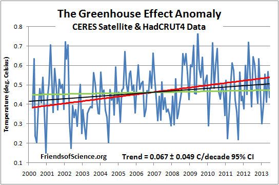

Studies published since 2010 indicates that equilibrium climate sensitivity is much
less that the 3 °C estimated by the IPCC in its 4th assessment report. A chart here
shows that the mean of the best estimates of 14 studies is 2 °C, but all except the
lowest estimate implicitly assumes that the only climate forcings are those
recognized by the IPCC. They assume the sun affects climate only by changes in
the total solar irradiance (TSI). However, the IPCC AR5 Section7.4.6 says,

 "Many studies have reported observations that link solar activity to particular
aspects of the climate system. Various mechanisms have been proposed that
could amplify relatively small variations in total solar irradiance, such as
changes in stratospheric and tropospheric circulation induced by changes in the
spectral solar irradiance or an effect of the flux of cosmic rays on clouds."

Many studies have shown that the sun affects climate by some mechanism other
than the direct effects of changing TSI, but it is not possible to directly quantify
these indirect solar effects. All the studies of climate sensitivity that rely on
estimates of climate forcings which exclude indirect solar forcings are invalid.

The IPCC AR5 report estimates the TCR to be likely (Box 12.2, Figure 2) in the
range of 1.0 to 2.5 °C, with a best estimate of 1.8 °C from climate models using a
CO2 growth of 1.0%/year. These estimates are unrealistic because they assume
no natural causes of climate change other than the changes in TSI and assume
that forcings and feedbacks used in climate models are correct. Fortunately, we
can calculate the transient climate response without an estimate of total forcings
or feedbacks by directly measuring the changes to the greenhouse effect (GHE).

Greenhouse Effect
The GHE is the difference in temperature between the earth's surface and the
effective radiating temperature of the earth at the top of the atmosphere as seen
from space. This temperature difference is generally given as 33 °C, where the
top-of-atmosphere global average temperature is about -18 °C and global average
surface temperature is about 15 °C. We can estimate climate sensitivity by
comparing the changes in the GHE to the changes in greenhouse gas
concentrations.

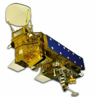
The Clouds and Earth's Radiant Energy
                                     System (CERES) experiment started
                                     collecting high quality top-of-atmosphere
                                     outgoing longwave radiation (OLR) data in
                                     March 2000. The last data available is June
                                     2013 as of February 23, 2014. Figure 1
                                     shows a typical CERES satellite.

Figure 1. CERES Satellite

The CERES OLR data presented by latitude versus time is shown in Figure 2.

Figure 2. CERES Outgoing Longwave Radiation, latitude versus date.

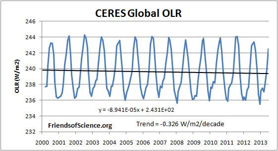
The global average OLR is shown in Figure 3.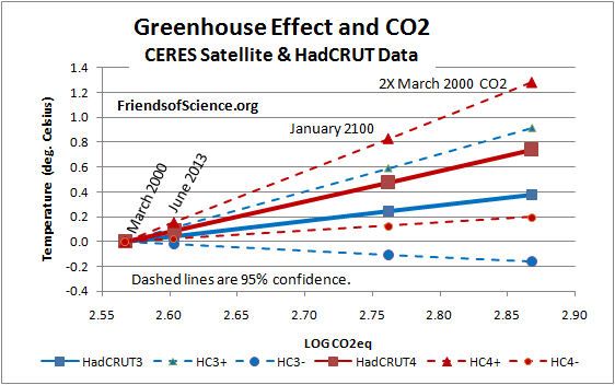

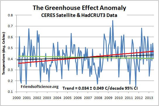
Figure 3. CERES global OLR.

The CERES OLR data is converted to the effective radiating temperature (Te) using
the Stefan-Boltzmann equation.

Te = (OLR/σ)0.25 - 273.15. where σ = 5.67 E-8 W/(m2K4), Te is in °C.

The monthly anomalies of the Te were calculated so that the annual cycle would
not affect the trend.

We use the HadCRUT temperature anomaly indexes to represent the earth's
surface temperature (Ts). The HadCRUT3 temperature index shows a cooling
trend of -0.002 °C/decade, and the HadCRUT4 temperature index shows a
warming trend of 0.031 °C/decade during the period with CERES data, March
2000 to June 2013. The land measurement likely include a warming bias due to
uncorrected urban warming. The hadCRUT4 dataset added more coverage in the
far north, where there has been the most warming, but failed to add coverage in
the tropics or in the far south, where there has been recent cooling, thereby
introducing a warming bias. We present results using both datasets.

The difference between the surface temperatures anomaly and effective radiating
temperature anomaly is the GHE anomaly. Figures 4 and 5 show the Greenhouse

effect anomaly utilizing the HadCRUT3 and HadCRUT4 temperature indexes,
respectively.

Figure 4. The greenhouse effect anomaly based on CERES OLR and HadCRUT3.

Figure 5. The greenhouse effect anomaly based on CERES OLR and HadCRUT4.

The trends of the GHE are 0.034 ± 0.049 °C/decade based on HadCRUT3, and
0.067 ± 0.049 °C/decade based on HadCRUT4 at 95% confidence. The black lines
show the best fit trends and the colored lines indicate the 95% confidence in the
trends.

No Feedbacks
In general, the monthly changes in OLR as measured by CERES includes the effects
of forcings and feedbacks in unknown quantities. Feedbacks are interactions
where a change in global surface temperatures cause a change in the radiation
budget, such as by changes in water vapor and clouds, that cause further
temperature change. There is no feedback if there is no temperature change. The
monthly changes in OLR would include changes from feedbacks, but this analysis
uses only the best fit trend during the entire CERES period when the temperature
trend was zero. Therefore, over the CERES era, any positive feedbacks were
match by negative feedbacks and there were no net feedbacks during the period.
The trend in OLR much be entirely due to changes in forcings as there was no
trend in temperatures and no net feedback over the period.

Non-greenhouse gas forcings must be equal and opposite to greenhouse gas
forcings to result in no temperature change over the CERES era. Both total
forcings and total feedbacks were zero over the period.

Greenhouse Gases Only Change the GHE
Changes in non-greenhouse gas forcings such as the sun's TSI, aerosols, ocean
circulation changes and urban heating can't change the GHE except by a feedback
that might change the water vapor amount. But as previously shown, during the
CERES era there was no temperature change, so there was no feedback-induced
change in water vapor. Changes in cloudiness could change the GHE, but data
from the International Satellite Cloud Climatology Project shows that the average
total cloud cover during the period March 2000 to December 2009 changed very
little. A change of TSI would change both the surface temperature (Ts) and the
effective radiating temperature (Te) equally, so there would be no change in the
GHE, which is Ts – Te in the absence of feedbacks. The GHE will change only if the
longwave absorption in the atmosphere changes, resulting in a change in the
downward longwave radiation. Changes in non-greenhouse gas forcings change
Ts and Te equally when there is no feedback-induced change in water vapor.

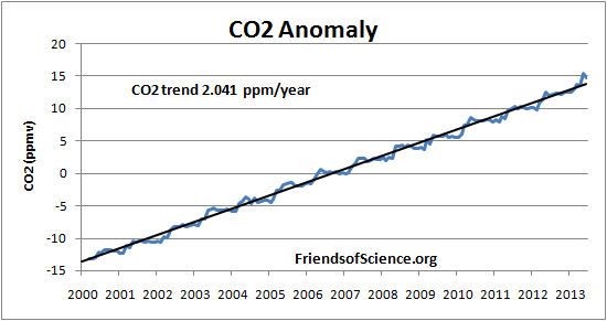
To further demonstrate this point, the HARTCODE line-by-line radiative code
program was used to calculate the change in Te resulting from a change in Ts. The
program calculates the surface fluxes, the atmospheric up and down longwave
fluxes, the LW window flux, the OLR etc. It includes a realistic water vapor profile
and greenhouse gases, which were held constant for this experiment. The results
show that a 1 °C increase in surface temperature caused the surface upward flux
to increase by 5.30 W/m2 and the OLR to increase by 3.79 W/m2, and increased
the effective radiating temperature by 0.97 °C. Therefore, non-greenhouse gas
forcings without feedbacks have an insignificant effect on the GHE = Ts-Te.

Therefore, we can conclude that the measured change in the GHE during the
CERES era is due to only anthropogenic greenhouse gas emissions, which is
dominated by CO2. We want to compare the trends in the GHE to changes in well
mixed greenhouse gases to determine the transient climate response.

Greenhouse Gas Forcing
The CO2 data also has a large annual cycle, so the anomaly is used. Figure 6 shows
the monthly CO2 anomaly calculated from the Mauna Loa data and the best fit
straight line.

Figure 6. CO2 anomaly.

Table 1 shows the radiative forcing of various greenhouse gases. CO2 changes in
the atmosphere accounts for 84.9% of the total GHG radiative forcing from the
year 2000 to 2012. Therefore, the total GHG forcing during the CERES era is the
CO2 forcing divided by 0.849.

    Year          CO2           CH4         N20         17-minor        Total
    2000         1.513         0.494       0.151          0.322         2.480
    2012         1.846         0.507       0.181          0.338         2.872
   Change        0.333         0.013       0.030          0.016         0.392
  % of total     84.9%          3%          8%             4%
Table 1. Changes in well-mixed greenhouse gas forcing in W/m2 relative to 1750,
and the change from 2000 to 2012.

The March 2000 CO2 concentration is assumed to be the 13 month centered
average CO2 concentration at March 2000, and the June 2013 value is that value
plus the anomaly change from the fitted linear line. Table 2 below shows the CO2
concentrations, the CO2 equivalent of all greenhouse gas changes, the logarithm
of the CO2 equivalent concentrations, and the change in the GHE from March
2000 for both the HadCRUT3 and HadCRUT4 cases. The change in the GHE is
proportional to the logarithm CO2 equivalent concentrations. We assume non-CO2
greenhouse gases do not change after June 2013.

Transient Climate Sensitivity

                                                           hadCRUT3 hadCRUT4
     Date         CO2      CO2eq      Log CO2eq      ΔF       ΔGHE       ΔGHE
                  ppm       ppm                    W/m2        °C          °C
 March 2000     368.88     368.88       2.567        0          0          0
  June 2013     395.94     400.94       2.603     0.4458      0.046      0.089
January 2100    572.68     577.67       2.762                 0.245      0.480
    2X CO2       737.76    737.76       2.868                0.379      0.741
Table 2. Extrapolated changes to the greenhouse effect (GHE) based on two
versions of the hadCRUT datasets.

Table 2 shows that the GHE has increased by 0.046 °C from March 2000 to June
2013 based on changes in the CERES OLR data and HadCRUT3 temperature data.
Extrapolating to January 2100, the GHE increase to 0.24 °C by January 2100. Using
the HadCRUT4 temperature data, the GHE increases by 0.48 °C by January 2100
compared to March 2000.

The last row of Table 2 shows the transient climate response (TCR), which is the
temperature response to CO2 concentration from March 2000 levels to the time
when CO2 concentrations have doubled. TCR is less than the equilibrium climate
sensitivity because the oceans have not reached temperature equilibrium at the
time of CO2 doubling.

In this analysis, TCR is calculated by the equation:

 TCR = F2x dT/dF ; whereF2x means the forcing due to a doubling of CO2
concentration, dT means the temperature difference of the GHE, dF means the
longwave forcing difference that would cause a change in the GHE, from March
2000 to June 2013.

In the common definition of TCR, dT is the air surface temperature change and dF
is the total forcing, including shortwave forcings. However, in this analysis, we
compare the change in the GHE to the forcings that cause that change. Only
longwave forcings can change the GHE, as shortwave forcings affect Ts and Te
equally.

 The CO2 forcing was calculated as 5.35 x ln (CO2/CO2i). The change in CO2 forcing
from March 2000 to June 2013 is 0.379 W/m2. The GHG forcing over the same
period was the CO2 forcing divided by 0.849, equal to 0.446 W/m2. The forcing for
double CO2 (F2x) is 3.708 W/m2. The TCR is 0.38 ± 0.54 °C using hadCRUT3, and
0.74 ± 0.54 °C using hadCRTU4 data. These values are much less than the multi-
model mean estimate of 1.8 °C for TCR given in Table 9.5 of the AR5. The climate

model results do not agree with the satellite and surface data and should not be
used to set public policies.

Figure 7 shows the results of Table 1 graphically. It also shows the 95% confidence
of the calculated temperature changes.

Figure 7. The greenhouse effect and CO2 extrapolated to January 2100 and double
CO2 bases on CERES and HadCRUT data.

This analysis shows that the temperature change from June 2013 to January 2100
due to increasing CO2 would be 0.20 ± 0.28 °C using HadCRUT3 or 0.39 ± 0.29 °C
using HadCRUT4, assuming the CO2 continues to increase along the recent linear
trend. If the two HadCRUT datasets are considered equally likely to represent
global temperatures, and assuming that CO2 emissions can't cause cooling, the
best estimate of CO2-induced global warming is 0.29 °C with a 95% confidence
range of 0.00 to 0.68 °C.

This estimate represents only the expected temperature change due to increasing
CO2 concentrations in the atmosphere. The effects of natural climate change
might be much greater than the CO2 effect. We know that natural climate change

caused a negative forcing equal and opposite to the positive greenhouse gas
forcing during the CERES era because there was no observed change in surface
temperatures.

Data and Calculations
An Excel spreadsheet with the data, calculations and graphs is here.
HadCRUT3 data is here.
HadCRUT4 data is here.
Mauna Loa CO2 data is here.
CERES OLR data is here.
Total cloud cover data is here.
Changes in radiative forcings is here.