Characteristics of high performing dairy farms in England

Characteristics of high
performing dairy farms in
England

Published: July 2020
Written by: Nicolas Jones
Enquiries to: Clare Betts
Department for Environment, Food and Rural Affairs
Email: FBS.queries@defra.gov.uk

1 Contents
1 Contents ...................................................................................................................... 1
2 Executive summary ...................................................................................................... 2
3 Introduction .................................................................................................................. 3
 3.1 Purpose and Definitions ........................................................................................ 4
 3.2 Data and Methodology .......................................................................................... 4
4 Results ......................................................................................................................... 5
 4.1 Breakdown of variation in performance.................................................................. 6
 4.2 Farm characteristics related to farming performance ............................................. 8
 4.2.1 Business decisions ....................................................................................... 10
 4.2.2 Farm characteristics ...................................................................................... 17
5 Conclusions ............................................................................................................... 22
6 Appendix A ................................................................................................................ 24
 6.1 Methods .............................................................................................................. 24
 6.1.1 Geographical and temporal variation in performance .................................... 24
 6.1.2 Factors related to farming performance ........................................................ 25
7 Appendix B ................................................................................................................ 26
 7.1 Spatial distribution of farm business output/input ratio ......................................... 26
 7.2 Model outputs ...................................................................................................... 27
 7.3 Model diagnostic plots ......................................................................................... 29
7. References ................................................................................................................ 29

 1

2 Executive summary
This report studies the characteristics of high performing dairy farms. Performance is
defined as economic performance measured by the efficiency with which inputs are turned
into outputs. The analysis covers the period 2010/11 to 2016/17 for dairy farms in England.
The first section of the analysis (section 3.1, below) compares the relative importance of
temporal, geographic and idiosyncratic (i.e. farm specific) factors in explaining variation in
the economic performance of dairy farms. Geographic factors, such as localised weather
and land quality, contributed very little to variation in performance, accounting for only
around 0.01% of variance. In contrast temporal (changes over time such as prices and
weather) and farm specific factors explained the majority of the variation in the data,
accounting for around 30% and 70% respectively. However, the influence of geographic
factors may have been underestimated due to data limitations, further details are in section
3.1.
The second section of the analysis (section 3.2) focuses mainly on farm specific factors
related to the performance of the farm business as a whole, and to the agricultural portion
of the business in isolation (i.e. excluding diversified income, direct payments and agri-
environment schemes). The results were categorised by those which the farm has control
over and those which are less controllable. Factors which were found to be related to
performance are listed below in Table 1.
Table 1. Factors which were found to be related to performance, indicates a positive relationship
with performance, indicates a negative relationship, and indicates no relationship. The size of
the arrow indicates the strength of the evidence, larger arrows indicating more confidence in the
result and smaller arrows indicating less confidence.
 Variable Farm Agriculture Comments
 Business
 Debt For both short and long term debt, increasing
 indebtedness was related to decreasing
 performance.
 Organic Organic dairy farms tended to be better
 performers than non-organic dairy farms, for
 both the farm business and the agricultural
 portion of the business.
 Agri- Increasing reliance on agri-environment
 scheme payments was associated with
 environment
 reduced agricultural performance, but this
 scheme
 was compensated for by the rest of the farm
 payments
 business such that overall performance was
 not impacted.
 Specialisation More specialised dairy farms preformed less
 well than those with a more varied
 agricultural enterprise, for both the farm
 business and the agricultural portion of the
 business.

 2

Diversification More investment in diversified activities was
 related to lower agricultural performance, but
 this was compensated for by the rest of the
 farm business such that overall performance
 was not impacted.
 Unpaid labour Unpaid labour was advantageous for
 performance. However, once the inherent
 advantage of receiving labour for free was
 removed by including an imputed cost, more
 unpaid labour was associated with reduced
 farm business performance.
 Herd size Farms which increased their herd size over
 the study period tended to be better
 performers than those whose herd has
 decreased.
 Tenure Tenanted, and in particular FBT (shorter)
 tenanted farms tended to have lower
 performance than FAT (more long term) and
 owner-occupied farms.

3 Introduction
There is substantial variation in the economic performance of farms in England, both
across and within sectors. Better understanding the causes of this variation is key for the
industry and policy makers to understand the drivers of productivity, competitiveness and
profitability. Farm performance is also often related to environmental outcomes. The
relationship between performance and farm characteristics is however often complex. This
is part of a series of three reports analysing factors related to economic performance at the
farm level.
Economic performance is a key measure of the productivity of farms and is defined as the
ability of farms to turn inputs into outputs. The dairy sector has the lowest difference in
performance between the best and worst performers of any agricultural sector in England
and yet variation is still extensive. In 2016/17 the top 25% performing farms in England on
average achieved £1.17 in outputs for every £1 spent on inputs whereas the lowest
performing 25% of farms only managed to achieve 81 pence in outputs for every £1 spent
on inputs1. In the same year only 46% of dairy farms broke even by achieving a return of
at least £1 for every £1 spent on inputs. When considering purely inputs and outputs
related to the agriculture aspect of the business only around 1 in 5 farms broke even.
The general trend in the structure of the dairy industry over the past decades has been towards
fewer but larger farms. In the decade between 2008 -2017, the number of holdings, total land area
and total cow numbers related to the UK dairy industry all fell; total land area by almost 20%
(Defra, 2019). Despite this reduction in key inputs, production increased by around 11% over the
same period, and the average land area per farm also increased, from 101 ha to 129 ha (Defra,
2019). At the industry level, the exiting of small farms from the industry, and the trend towards

1
 Farm Business Survey data 2016/17
 3

larger farms has been presented as the key driver of industry productivity growth (Kimura and
Sauer 2015); the suggestion being that larger farms are able to benefit from returns to scale. At the
individual farm level however a number of factors are likely to explain the variation in the economic
performance of dairy farms.

3.1 Purpose and Definitions
The purpose of this report is to provide an up to date assessment of the characteristics
associated with economic performance for dairy farms in England. The analysis within this
report was produced alongside (Betts, 2020) and (Jones, 2020) which analyse the grazing
livestock and cereals sectors respectively.
Economic and financial performance of farms can be measured using a number of
different indicators. This report focuses on efficiency; specifically technical efficiency.
Technical efficiency is defined as how much output a farm can produce per unit of input. In
this study outputs are measured as the monetary value of products produced by the farm.
Inputs are measured as all monetary costs to the farm in addition to an amount
representing unpaid family labour. Although unpaid labour does not appear on a farm’s
balance sheet, it represents a financial cost to the farm through forgone off-farm wages.
Where a cost for unpaid labour was used this was done using the market rate and
represents what a worker could have earned doing the same job elsewhere. This is not a
perfect measure as many farmers have the skills and qualifications to earn a higher wage
in another sector. On the other hand farmers receive a number of non-monetary benefits
such as housing, and lifestyle benefits which they value highly. These benefits offset lost
earnings to an extent.
Inputs and outputs were not deflated to account for changes in prices over time. This is to
allow for a wider definition of efficiency which includes allocative as well as technical
efficiency. Where technical efficiency considers how a product is made, allocative
efficiency relates to which products should be made. Allocative efficiency is defined as the
best mix of goods being produced. Price changes have an impact on allocative efficiency;
if input prices change, the most appropriate combination of inputs and outputs also
changes. For instance, if the cost of fertiliser falls in a given year, farmers may apply more
fertiliser to benefit from cheaper production costs and achieve higher output. This may
make allocative sense, however may lead to reductions in technical efficiency. In practice
changes in price over time are captured within the model by the inclusion of a “year”
variable.

3.2 Data and Methodology
A simplified explanation of the data and methods used in the analysis is presented here. A
more detailed technical breakdown of data and methods used can be found in Appendix A.
Data was taken from the Farm Business Survey2 of England for 2010/11 – 2016/2017.
Farms were included in the analyses if their farm type3 was classified as dairy in at least

2
 https://www.gov.uk/government/collections/farm-business-survey
3

https://assets.publishing.service.gov.uk/government/uploads/system/uploads/attachment_data/file/365564/fb
s-uk-farmclassification-2014-21oct14.pdf
 4

three of these years and they had at least 20 dairy cows. 328 farms met these conditions,
of which 164 were surveyed in all seven years and 250 in at least five. The majority (96%)
of farms were always classified at dairy, with the remainder classified as mixed or grazing
livestock for some years.
Within the Farm Business Survey, each farm business is broken down into four ‘cost
centres’; agriculture, diversification, direct payments and agri-environment schemes. Costs
and outputs are apportioned as appropriate between these cost centres. All the analysis in
this report has been produced using both farm business costs and outputs (i.e. including
all cost centres), and also for the agricultural portion of the business alone.
The analysis is split into two sections. The first section uses the ratio of outputs to inputs to
understand how much of the variation in economic performance can be attributed to the
location of each farm (i.e. large scale geography), changes in time (e.g. price changes
from year to year, or agricultural policy changes) and how much can be attributed to
‘idiosyncratic’ factors which are specific to each farm.
The second section of the analysis uses generalised linear mixed models to further
analyse the characteristics associated with farming performance. In this section putative
relationships between a number of factors and performance are tested. Costs, herd size
and land area were included in the model to take into account differences in farm size.
Two separate models were run to determine factors affecting purely the agricultural part of
the farm business and those affecting the business as a whole.
All results presented in the second section are in the form of model predictions, which
allow us to draw conclusions about the relationship between a farm/farmer characteristic
and economic performance, once the impact of other variables have been accounted for.
Predictions of outputs (the response variable used) were then divided by inputs to convert
the model predictions into estimates of performance. In all instances, predicted values
should be treated with caution since they are an estimation made based on a combination
of average values of the other variables, which may not be representative of actual farms,
and it would be uninformative to compare absolute predicted values across different
pieces of analysis (i.e. those relating to other farm types), instead, consider the directional
relationships between significant variables and economic performance as an indicator of
the nature of the relationships.
The analysis presented here is principally directed towards identifying correlations and
patterns in the data, and should not be used to infer causation. That two variables are
highly correlated to one another does not mean that one is driving change in the other. It is
also possible that other factors not included in the model are driving the results, despite
every effort being made to reduce this possibility. As well as the results from the data
analysis, theory and external evidence must be used to build a narrative to explain
possible causation. This is reflected in the interpretation of the results.

4 Results
The analysis is in two sections; the first examines how much of the variation in economic
performance can be attributed to the location of each farm (i.e. large scale geography),
changes in time (e.g. price changes from year to year, or agricultural policy changes) and

 5

how much can be attributed to factors which are specific to each farm. This final driver of
performance – farm characteristics – is further explored in the second phase of analysis.

4.1 Breakdown of variation in performance
There are numerous factors which may explain the variation in economic performance of
farms in England, however these can largely be categorised into three main groups:
geographic, temporal and characteristics which are specific to each farm.
Geographic factors are those which are unique to farms in a particular region or area of
the country. This could be regional differences in climate or land quality. Temporal
variations are changes in performance occurring over time and explain why the same farm
may appear to perform less well one year compared to the next. Temporal factors include
changes in prices and extreme weather events. Lastly, characteristics which are specific to
each farm explain why farms located in the same region, and compared within the same
timeframe still show variation in economic performance. This can be due to decisions
made by the farmer, as well as more local geographic differences such as grass quality.
This section discusses the results from the first part of the analysis which determines the
contribution of these three overarching sources of variation in economic performance
within the data.
Figure 1 shows the spatial distribution of farm performance for dairy farms for the years
2010/11 – 2016/17 (see Figure 15, Appendix B, for the farm business distribution). Here
farms are grouped into quintiles based on their average performance. The overall
distribution of points reflects the general trend for the highest density of dairy farms in
England to be in the West, particularly in counties such as Devon, Cheshire and
Lancashire. The distribution of performance is reflected by the colour of the points; the
majority of areas appear to have a mix of high and low performing farms, again suggesting
that geographic area only explains a minimal amount of the variation in performance.
Some systematic differences in performance between years can be seen in Figure 2. This
shows the annual average performance of dairy farms for the years within this study and
with earlier years taken from Langton (2013).

 6

Figure 1. Spatial distribution of output/input ratios calculated from agricultural inputs and outputs
only. Mean performance for farms falling within each 10km grid square are shown.

Figure 2. Farm business performance of dairy farms (calculated as the ratio of outputs to inputs
(including an imputed costs for unpaid labour)) has not changed systematically over time. Previous
work (Langton, 2013) covers the years 2003/04 – 2009/10, current analysis covers the years 2010/11 –
2016/17. Values shown are the median ratio for dairy farms in each year.

 7

The main source of variation in economic performance was found to be characteristics
associated with individual farms (Table 2), making up 69% and 70% of variation in
performance in the farm business and agricultural models respectively. Temporal factors
were also important, with annual changes shown to contribute 31% to variation in farm
business efficiency and 29% to agricultural efficiency. In contrast geographic factors were
relatively inconsequential and only accounted for around 0.1% of variation. These will
likely be underestimates due to the limited geographic information available for FBS farms;
the location of FBS farms is only known to the nearest 10km, and small scale geographical
differences such as elevation, or soil quality is poorly reflected by NCA designations and
will instead be accounted for by the variation between farms variable. But the geographic
variation it is nevertheless much lower than year to year variation within farms, and farm to
farm variation. It is important to emphasise that this result does not necessarily mean that
geographic differences in economic efficiency do not exist, but rather that the FBS dataset
is not sensitive enough to pick them up. Indeed, the very fact that dairy farms tend to be
concentrated in the West of the country reflects the fact that geography is important. Even
where a few farms exist outside the core dairy areas, the geographic trend may be
obscured if, as is likely, these dairy farms are highly motivated and manage to deliver
profits despite the disadvantages of their geographic location.
Table 2. Sources of variation within the dataset
 Farm business Agriculture
 Component Variance % of total Variance % of total
 Geographical variation (NCA) 0.07 0.1 0.07 0.1
 Farm to farm variation 54.87 69.1 54.45 70.6
 Year to year variation within farms 24.43 30.8 22.64 29.3

4.2 Farm characteristics related to farming performance
In the previous section the relative importance of farm specific differences in explaining
variation in economic performance was demonstrated. This section takes a more detailed
look at the farm specific factors to better understand the characteristics of higher
performing farms. For the modelling in this section, the relationship between monetary
inputs and monetary outputs was considered, alongside other variables which may
influence that relationship. A variety of variables and their interactions were used in the
modelling, chosen largely on the basis of theory, or for data quality. For instance, it was
not possible to include some variables relating to business management practices (e.g. the
use of financial plans) because these data was not collected for all farms, resulting in a
very small sample size. For a full list with descriptions see Table 5 in Appendix A.
Two different models are used here. The first includes all farm business costs and outputs,
whereas the second only includes inputs and outputs related to agricultural production.
The former gives an indication of the overall economic and financial performance of the
farm business and includes income related to subsidies and diversified parts of the
business. By also including the latter model, comparison can be made between factors
which impact agricultural performance, and those which have an impact on the
performance of the business as a whole. Many of the variables considered have a similar

 8

relationship with performance in both models; more so than in the cereals (Jones, 2020)
and grazing livestock (Betts, 2020) studies. This is explained by the fact that dairy farms
tend to receive a high proportion of their income from agriculture rather than other income
types such as diversified enterprises. This is worth keeping in mind when interpreting the
results.
The results in this section are structured so as to make a distinction between those factors
which are within the control of the farmer and those that are less controllable. This is a
somewhat arbitrary dichotomy as most of the factors are not fully controllable or
uncontrollable, however categorising in this way is useful for understanding the application
of the results. The variables included in the model are limited to those found in the Farm
Business Survey (FBS), which although a vast dataset, does not include all variables
which may be worth considering.
Table 3 lists the variables in each model along with their respective f-values and p-values.
A more detailed results table and variable definitions can be found in Appendices A and B.
Table 3. Variables found to be related to either farm business or agricultural performance. See Table
5 in Appendix A for the full list of variables considered and their descriptions. P-values are in bold
where variables were found to be related to either farm business or agricultural performance.
 Farm business Agricultural
 performance performance
 F-value P-value F-value P-value
 Specialisation 23.5

treated with caution since they are estimated at a combination of average values of the
other variables which may not be realistic in practice.

4.2.1 Business decisions
This section concentrates on variables which may affect economic performance, which are
particular to each farm in each year. Here we concentrate on variables which might be
thought of as business decisions and which are amenable, at least in theory, to change.
Further on we consider some variables which are largely beyond the scope of a farmer to
change.

4.2.1.1 Dairy Specialisation
Specialisation was calculated using the percentage of total Standard Labour Requirement
(SLR) attributed to dairy production. There was a negative relationship between
specialisation and performance for both the farm business and agricultural portion of the
business (see Figure 3).
This was similar to findings by (Langton, 2013) as well as other UK studies (Hadley, 2006)
but is in contrast to Barnes et al (2010) and Redman et al (2018) who find that
specialisation increases performance in dairy farming. Arguably, the latter relationship is
as expected due to the increasing requirement to use specialised machinery and workers
within the dairy sector (Barnes, et al., 2010). The results in this study do not necessary
contradict previous analysis, however contrasting results across studies suggest there
may be a complex relationship.
Redman et al. (2018) propose that farms who produce their own inputs such as forage and
youngstock may perform better than those who do not as inputs will be more bespoke and
appropriate for the specific characteristics of that farm. Inputs may also be better quality as
farms are likely keep the best for themselves and sell the excess. The calculation of
specialisation in this study uses a narrow definition of dairy production which does not
include input production, thus it is possible that some of those less specialised farms which
are better performers, may devote more resources to producing their own inputs.
Alternatively, less specialised farms may be more buffered to changeable markets and so
generate higher incomes on average.

 10

Figure 3. The relationship between specialisation and performance for both the farm business and
agriculture models. Predictions were made for an average farm with £320k inputs per annum, 130
cows and 100 ha of land, remaining variables were averaged or the most common factor level used.
Error bars represent standard error. Absolute predicted values should be treated with caution since
they are estimated at a combination of average values of the other variables which may not be
realistic in practice.

4.2.1.2 Diversification
Whereas specialisation refers to specialising within agriculture, diversification relates to
activates outside of the core agricultural business, such as tourism or renting out farm
buildings, but which utilise the farm’s resources. Diversification was calculated as the
percentage of farm business costs related to diversified activities.
Increasing diversification was related to slightly lower agricultural performance, and no
relationship was found between diversification and farm business performance (see Figure
4). It is possible that diversifying pulls focus and recourses away from the agricultural
share of the business, which then suffers as a result. That there was no relationship
between diversification and farm business performance suggests that any lost agricultural
output is made up for through diversified activities. Alternatively poor performing farms
may be forced to seek diversified income to remain competitive.

 11

Figure 4. The relationship between diversification and performance for both the farm business and
agriculture models. Predictions were made for an average farm with £320k inputs per annum, 130
cows and 100 ha of land, remaining variables were averaged or the most common factor level used.
Error bars represent standard error. Absolute predicted values should be treated with caution since
they are estimated at a combination of average values of the other variables which may not be
realistic in practice.

4.2.1.3 Organic
Organic farms were defined as those with 50% or more of farmed land under organic
certification. In practice however, dairy farms tend to be highly specialised as organic or
non-organic. Within the sample 75% of farms in the organic category used at least 96% of
their land for organic purposes. In contrast, the average non-organic farm in the sample
used less than 1% of their land to produce organic output.
Organic farming was associated with higher farm business and agricultural performance
(see Figure 5). In general, organic farms tend to have lower yields than non-organic farms
(Seufert, 2012). This means that an organic farm would produce less milk than a non-
organic farm with the same herd size. The results in this study suggest that even if the
volume of milk produced by organic farms is lower than a non-organic farm, the total value
of milk output is higher than non-organic farms of the same size, this is unsurprising given
that organic milk commands a higher price than non-organic milk, which compensates
organic farmers for the extra inputs needed to produce a litre of milk.

 12

Figure 5. The relationship between organic farming and performance for both the farm business and
agriculture models. Predictions were made for an average farm with £320k inputs per annum, 130
cows and 100 ha of land, remaining variables were averaged or the most common factor level used.
Error bars represent standard error. Absolute predicted values should be treated with caution since
they are estimated at a combination of average values of the other variables which may not be
realistic in practice.

4.2.1.4 Debt
Debt was disaggregated into short and long term debt, to distinguish between borrowing
for long term investments (such as bank and family loans) and borrowing to pay short term
bills (e.g. overdrafts, hire purchase and leasing costs).
Greater levels of debt were associated with poorer performance, for both short and long
term debt, and for both the farm business and the agricultural portion of the business (see
Figure 6). It is possible that the financial constraints faced by indebted farms restrict their
ability to adjust to changing markets or make investments and thus reduces their
performance. It is also possible that poorer performing farms are forced into greater levels
of debt to their cover unexpected shortfalls in income. The degree of variability in the data
is an important consideration here: there were many instances of farms with moderate
levels of debt performing well, and equally of farms with very little debt which were
amongst the poorest performers.
Previous studies have found contradictory relationships between debt and performance.
Langton (2013) found that farms with higher levels of debt tended to be poorer performers.
In contrast, Barnes et al. (2010) found a positive relationship between debt and
performance. Theoretically debt is likely to have two main purposes: farms borrow to make
efficiency boosting investments or to expand; or borrowing is used to supplement earnings
where cash flow is an issue. The former would be expected to lead to increased efficiency,
whereas the latter could be a sign of a poor performing farm.

 13

a) b)

Figure 6. The relationship between short term (a) and long term (b) debt, and performance for both
the farm business and agriculture models. Predictions were made for an average farm with £320k
inputs per annum, 130 cows and 100 ha of land, remaining variables were averaged or the most
common factor level used. Error bars represent standard error. Absolute predicted values should be
treated with caution since they are estimated at a combination of average values of the other
variables which may not be realistic in practice.

4.2.1.5 Unpaid Labour
Unpaid labour was included as a cost and calculated using the market rate for similar
agricultural work off the farm. This removes the inherent advantage of receiving labour at
no cost and acknowledges the true cost to the farm of unpaid labour. The percentage of
labour which was unpaid was also included in the analysis. As the percentage of unpaid
labour increased the performance of the farm business decreased (see Figure 7a). This is
in line with findings by Barnes et al. (2010) but contrasts to those by Langton (2013).
Langton (2013) found that unpaid labour has a positive relationship with agricultural
performance only when calculated at the minimum wage. When the market rate is used
the relationship no longer exists.
When the imputed cost for unpaid labour was removed from the analysis, a greater
reliance on unpaid labour was associated with increased farm business performance (see
Figure 7b). This relationship makes sense as without removing the advantage gained by
free labour, those with more unpaid labour will appear to be more efficient.
The relationship between unpaid labour and performance is a complicated one. Barnes et
al. (2010) propose that paid labourers may be more specialised leading to greater labour
efficiency, and Redman et al. (2018) suggest that unpaid labour may be more likely to do
low-value work, and hence have low productivity. In contrast Langton (2012), in the
context of grazing livestock farms, argued that family labourers have more of a stake in the
success of the business which could lead them to be more productive than paid labourers.
The true relationship is likely to be more nuanced with the relationship depending on other
factors such as the skill level of paid and unpaid workers. As pointed out by Barnes (2010)
the FBS is unable to provide enough detail to further explore this fully.

 14

a) b)

Figure 7. The relationship between unpaid labour and agricultural performance including an imputed
cost (a) and excluding an imputed cost (b). Predictions were made for an average farm with £320k
inputs per annum, 130 cows and 100 ha of land, remaining variables were averaged or the most
common factor level used. Error bars represent standard error. Absolute predicted values should be
treated with caution since they are estimated at a combination of average values of the other
variables which may not be realistic in practice.

4.2.1.6 Agri-Environment Scheme Payments
Payments from agri-environment schemes as a percentage of income was related with
lower agricultural performance (see Figure 8). This is unsurprising as by design agri-
environment schemes encourage farmers to forgo a certain amount of output to produce
environmental outcomes. No relationship was found between agri-environment scheme
payments and farm business performance. This suggests that agri- environment payments
are priced at the correct level so to act as income forgone and not disadvantage farms
financially for participating.

 15

Figure 8. The relationship between agri-environment scheme payments and agricultural
performance. Predictions were made for an average farm with £320k inputs per annum, 130 cows and
100 ha of land, remaining variables were averaged or the most common factor level used. Error bars
represent standard error. Absolute predicted values should be treated with caution since they are
estimated at a combination of average values of the other variables which may not be realistic in
practice.

4.2.1.7 Herd size
Herd size was found to have a positive relationship with both farm business and
agricultural performance (see Figure 9a), suggesting that a farm with more dairy cows but
the same land area and costs, produce farm business and agricultural output more
efficiently.
A variable for the trend in herd size was also included in the analysis. This variable
measures whether farms have generally expanded or reduced their herd size over the
period studied. Farms which had expanded their herd size tended to have higher
performance than those who had reduced their herd size (see Figure 9b). It is not clear
whether increased performance is attributable to expanding the business or whether those
with higher performance are better positioned to expand.

 16

a) b)

Figure 9. The relationship between herd size (a) and the trend in herd size (b) and performance for
both the farm business and agriculture models. Predictions were made for an average farm with
£320k inputs per annum, 130 cows and 100 ha of land, remaining variables were averaged or the
most common factor level used. Error bars represent standard error. Absolute predicted values
should be treated with caution since they are estimated at a combination of average values of the
other variables which may not be realistic in practice.

4.2.2 Farm characteristics
This section concentrates on variables which may affect economic performance, which are
particular to each farm in each year. Here we concentrate on variables which are largely
beyond the scope of a farmer to change.

4.2.2.1 Tenancy
Here farms were grouped into mainly owner occupied and mainly tenanted. Those in the
tenanted category were then spilt into those renting mainly under Full Agricultural Tenancy
(FAT) and those under Farm Business Tenancy (FBT) agreements.
Tenure type was related to both farm business and agricultural performance. On average,
FBT farms performed less well than owner occupied and FAT farms for both farm business
and agricultural performance (see Figure 10). This could be because the costs included in
the models do not include an imputed rent for owner-occupiers, but do include the actual
rent paid by tenants. When an imputed rental value for owner-occupied land was included
in the models, a similar but less pronounced pattern emerged, suggesting that the
differences were driven by more than just the cost of renting land. Some of this effect
could also be due to the relative security of the two tenancy types. FATs tend to come with
lifetime tenure and often include succession rights. In contrast FBT contracts tend to be
much shorter. The Central Association of Agricultural Valuers (CAAV) for example
estimate that the average new FBT agreement in 2016 was under 5 years 4. Farms with a
greater security of tenure may be more willing to make long term efficiency boosting
investments as they are better able to appropriate the full benefits of these investments.

4
 When contracts under 1 year are excluded this rises to around 6 years. The CAAV also acknowledge that
this is likely to be an underestimation however it still serves the purpose of demonstrating the vast difference
in contract length between FAT and FBT agreements on average.
 17

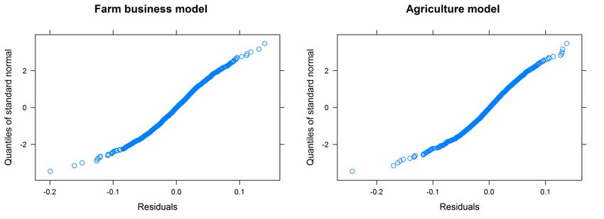
Figure 10. The relationship between tenure and performance for both the farm business and
agriculture models. Predictions were made for an average farm with £320k inputs per annum, 130
cows and 100 ha of land, remaining variables were averaged or the most common factor level used.
Error bars represent standard error. Absolute predicted values should be treated with caution since
they are estimated at a combination of average values of the other variables which may not be
realistic in practice.

4.2.2.2 Returns to scale
The recent trend in the UK dairy industry is of increasing average land area and herd size,
while yields have also increased. Over the same period the number of holdings has
declined. The industry is therefore characterised by fewer, larger farms producing more
milk. This is reflected in the FBS sample used in this analysis. Figure 11 shows that
median farm size has generally increased over time within the sample. Previous analysis
suggests that these structural changes have been a key contributor to increased efficiency
in the industry. Kimura and Sauer (2015) propose that the increase in average farm size
and the exit of smaller farms from the industry has been the most important factor in
explaining productivity growth in the UK dairy industry over the past two decades. Studying
the agricultural sector as a whole, Thirtle et al. (2004) found that a 1% increase in average
farm size led to a 0.2% increase in UK agricultural productivity.

 18

Figure 11. Box plot of land area (Ha) for dairy farms in the FBS from 2003/04 – 2016/17.

Although farms of a similar size will vary in their levels of costs, land area and herd size, a
significantly larger farm will have more of all three. A useful way of understanding the true
relationship between scale and performance is to consider the impact of a proportionate
increase in these variables concurrently. This gives an indication of whether there is
increasing returns to scale in the industry. Figure 12 shows the predicted change in
performance from a change in land area, herd size and costs of 10%. Constant returns to
scale, a scenario where output changes proportionately with inputs, is represented by the
line. The graph shows that performance changes by more than 10% if the scale variables
are changed by 10% which suggests the existence of increasing returns to scale.

Figure 12. Predicted performance change from decreasing and increasing land area, herd size and
costs by 10%. The line represents constant returns to scale. Error bars represent standard error.
Absolute predicted values should be treated with caution since they are estimated at a combination
of average values of the other variables which may not be realistic in practice.
 19

Previous work (Langton, 2013) has also found evidence of increasing returns to scale for
all but the largest dairy farms suggesting that an optimum size exists at which further
growth will no longer lead to increased performance. It is worth noting however that other
past studies have found mixed results when analysing whether increasing returns to scale
exists in the UK dairy industry. For example Hadley (2006) found slight increasing returns
to scale, whereas Barnes et al. (2010) found constant returns, suggesting farms are
already operating at their optimum level on average, and Barnes (2008) found diminishing
returns to scale for dairy farms in Scotland.

4.2.2.3 Year
The year variable was included in the analysis to control for annual fluctuations in
performance across farms due to in year impacts, such as changes in prices or extreme
weather events.
The annual fluctuations in farm business and agricultural performance across farms is
shown in Figure 13. 2011 and 2013 appear to be particularly good years for the industry
with relatively high performance. In contrast performance is particularly low in 2015 and
2016. Farm business and agricultural performance follow similar trends reflecting the
importance of agricultural income to total farm income.

Figure 13. The relationship between year and performance for both the farm business and agriculture
models. Predictions were made for an average farm with £320k inputs per annum, 130 cows and 100
ha of land, remaining variables were averaged or the most common factor level used. Error bars
represent standard error. Absolute predicted values should be treated with caution since they are
estimated at a combination of average values of the other variables which may not be realistic in
practice.

A number of factors will contribute to annual fluctuations in the income of a dairy farm
however milk prices are arguably the most important for the dairy industry. The importance
of milk prices can be seen clearly in Figure 14 which compares agricultural performance to

 20

average annual UK milk prices. Predicted output and milk prices follow a very similar
trend, travelling in the same direction for all but one year. This suggests that milk prices
are important in explaining yearly variation in the model. Disentangling the causes of
variations in milk prices is complex however weather, livestock disease, foreign trade and
consumer tastes are all likely to contribute. Arguably one the most important influencers of
milk prices over the period studied however are EU milk quotes which ceased in 2015
leading to falls in milk prices over the subsequent years. This is likely to explain much of
the fall in output of farms within the study in 2015 and 2016.

Figure 14. The relationship between year and agricultural costs (top) and annual UK milk prices
(bottom). Predictions were made for an average farm with £320k inputs per annum, such that
differences in the y-axis (outputs) can be interpreted as difference in performance. The ‘average
farm’ also had 130 cows and 100 ha of land, remaining variables were averaged or the most common
factor level used. Absolute predicted values should be treated with caution since they are estimated
at a combination of average values of the other variables which may not be realistic in practice.

 21

5 Conclusions
The first section of the analysis aimed to determine the relative importance of three main groups of
factors in explaining the variance in economic performance of dairy farms in England. The results
suggested that geographic factors are relatively unimportant, however this may be partly due to
limitations in the data. Temporal factors had a clear impact on variation, and farm specific factors
explained the majority of variation in economic performance within the sample analysed.

In the second, and main, section of the results, farm specific factors were tested to better
understand the characteristics of higher performing farms. The conclusions are summarised below.

Table 4. A summary of the results with comment on the strength of the evidence.
 Variable Evidence Strength Comments
 Specialisation Moderate – similar Agricultural specialisation was associated
 and contrasting with lower performance
 patterns have been
 reported elsewhere.
 Diversification Moderate – similar More investment in diversified activities was
 patterns have been related to lower agricultural performance, but
 found in other this was compensated for by the rest of the
 systems and farm business such that overall performance
 previous studies. was not impacted.
 Organic Strong - this pattern Farms which had a larger proportion of land
 has been reported under organic certification tended to better
 elsewhere. performers.
 Debt Strong – this pattern For both short and long term debt, increasing
 has been found indebtedness was related to decreasing
 across many performance.
 systems and studies.
 Unpaid labour Moderate – similar Unpaid labour was advantageous for
 and contrasting performance. However, once the inherent
 patterns have been advantage of receiving labour for free was
 reported elsewhere. removed by including an imputed cost, more
 unpaid labour was associated with reduced
 farm business performance.
 Agri- Strong - this pattern Increasing reliance on agri-environment
 environment has been reported scheme payments was associated with
 scheme elsewhere. reduced agricultural performance, but this
 payments was compensated for by the rest of the farm
 business such that overall performance was
 not impacted.
 Herd size Strong - this pattern Farms which had larger herd sizes tended to
 has been reported be better performers.
 elsewhere.
 Change in herd Moderate - similar Farms which increased their herd size over
 size patterns have been the study period tended to be better
 found previously. performers than those whose herd has
 decreased.

 22

Tenure Moderate - similar Tenanted, and in particular FBT (shorter)
 patterns have been tenanted farms tended to have lower
 found in other performance than FAT (more long term) and
 systems and owner-occupied farms.
 previous studies.

Farm specific factors were categorised into those which farmers are to some extent able to control,
and those that are more difficult to change. Although this categorisation is not perfect, it does
demonstrate that there are a number of key factors related to performance which are under the
control of the farmer. This suggests that there is at least some potential for lower performing farms
to improve their performance.

This conclusion must however be accompanied by some key caveats. Firstly, just because
a variable considered here doesn’t appear to have a relationship with performance, does
not necessarily mean that it is unrelated. All statistical analysis is limited by the sample
size of the data considered, with more data comes more power to detect relationships.
Subtler, or nuanced, relationships may not be picked up by the models.
Secondly, it is important to recognise that economic performance is not the only consideration for
farmers. From a financial perspective farmers may be more interested in farm business income
(net profit) as this is likely to more directly impact their personal consumption. More significantly,
financial incentives may not be the primary concern to farmers. Farmers gain a number of non-
monetary benefits from farming, such as ability to live a particular lifestyle. Maintaining this lifestyle
may be more of a concern than cultivating an efficient, profit making business. Therefore while it
may be possible for farmers to improve the economic performance of their farm, they may not have
the desire to do so.

Policy makers must also be aware of the complex relationships between efficiency and
productivity gains and other policy aims such as improving environmental outcomes. Much
historic productivity growth in agriculture can be attributed to the substitution of labour for
energy intensive machinery, as well as growth in the use of fertilisers and pesticides.
These inputs tend to have a number of negative environmental consequences associated
with them. Depending on the nature of gains, the move towards greater efficiency on farms
has the potential to either exacerbate or mitigate environmental degradation. Foster et al.
(2007) show that there are often trade-offs between reducing one negative input and
another. For example using less fertiliser will have positive environmental impacts but will
require the use of more land to produce the same amount of output. Using more land for
agriculture can have negative impacts on biodiversity and also represents the loss of land
which can be used for carbon capture through woodland. There are indications however
that increased efficiency will also lead to environmental benefits in the dairy sector.
Shortall and Barnes (2013) found that more efficient Scottish dairy farms also produce less
greenhouse gasses per litre of milk produced, although they acknowledge that how
efficiency gains are achieved is hugely important. Previous work has been done to widen
measures of productivity to include environmental outcomes however these measure as
not yet mainstream5.

5
 For example see (Thirtle & Holding, 2003) paper 5 which calculates a Total Social Factor Productivity
(TSFP) index for the UK farming industry. Alternatively Total Resource Productivity (TRP) – see (Gollop &
Swinand, 2001).
 23

6 Appendix A

6.1 Methods
Data was taken from the Farm Business Survey of England for 2010-2016. Farms were
included in the analyses if they were ‘robust’ type dairy farms in at least three of these
years, of which 329 fit this criteria. Farms were also required to have more than 20 cows to
be included in the sample. This left a sample of 328 farms. 164 of these farms were
surveyed in all seven years, with 250 surveyed in at least five of the seven years. 96% of
farms were always classified as dairy, with the remainder classed as either grazing
livestock or mixed for some years.
The data was checked for anomalies and no further farms were removed.
Unpaid labour was given an imputed cost equivalent to the amount that the unpaid staff
could earn in similar work elsewhere. Rent was not imputed for owner occupied farms.
Statistical analysis was broken up into two sections; the first using two models to assess
the spatial and temporal variation in farm input/output ratios, the second assessing
variables which might be associated with the economic performance at the farm business
level, and agricultural portion of the business only. The farm business accounts includes
costs and outputs from traditional farming sources, as well as diversified activities (such as
tourism or renting out buildings), direct payments from government and payments from
agri-environment schemes.
All statistical analyses were done in R (R Core Team, 2018), using the lme function in the
nlme package (Pinheiro, et al., 2018) to fit mixed effects models. For both the farm
business and agriculture models, farm ID was fitted to have a random effect on the
intercept. Models were fitted using Maximum Likelihood during model simplification, and
Restricted Maximum Likelihood to obtain final coefficient estimates.
Response variables were either log transformed farm business outputs, or log transformed
agricultural outputs (both in whole £000s).

6.1.1 Geographical and temporal variation in performance
To partition the variation in performance between geographical (using Joint Character
Areas), temporal (year) and idiosyncratic (farm ID) sources, a simple ANOVA was used
taking the form:
 ~ Farm/Year + NCA

Where performance ratio refers to the input/output ratio for the farm business and
agriculture respectively, and NCA refers to the National Character Area. Each dependant
variable was fitted as a factor. Government Office Regions (GOR) were also used in the
place of NCA but this made no meaningful difference to the results.
To visualise the spatial distribution of performance, for each 10km grid square across
England, an average performance score was calculated, where data existed. These
scores were then categorised into bands (bottom 20%, 21-40%, 41-60%, 61-80% and top
20%) and plotted.
 24

6.1.2 Factors related to farming performance

6.1.2.1 Fixed effects structure
Generalised linear mixed models were used to assess other putative explanatory variables
associated with farm business and agricultural performance, taking the general form:
 log( ) ~ 0 + log( ) + year + log( ) + 1 + ⋯ + + farm
 + ε

Where;
  log(outputs) and log(costs) are log transformed outputs and costs in whole
 thousands of pounds.
  β0 is a global intercept
  year is a categorical variable denoting each year
  log(area) is log transformed total area, including woodland, buildings etc.
  variable1 … variablen are additional variables
  farm is fitted to have a random effect on the intercept
  ε is residual error
The full list of variables used:
Table 5. List of variables with summary statistics.
 Variable Description Min Max Mean/mode
 (log) output Log10 farm business 1.6(1.55) 3.34(3.29) 2.54(2.49)
 (agricultural) output
 (Log) costs Log10 farm business 1.73(1.73) 3.32(3.3) 2.53(2.52)
 (agricultural) costs
 (log) area Log10 land area 1.37 3.1 2.06
 (log) herd size Log10 dairy cow herd size 1.4 2.82 2.1
 Dairy cow trend Trend in herd size Small Increase
 Unpaid labour Percentage of labour which is 0 73.58 15.78
 unpaid
 Tenure Owner occupied if 50% or more Owner
 of land owned, otherwise Occupied
 tenanted. For tenanted, FAT if
 50% of tenanted land under
 FAT, otherwise FBT.
 Specialisation Percentage of SLR related to 31.45 96.92 70.48
 dairy production
 Diversification Percentage of costs related to

The same maximal model was fitted to both the farm business data and the agricultural
data, and potential fixed effects were assessed on the basis of stepwise model
simplification (Crawley, 2013), model AIC and model performance. No automated model
simplification or variable selection procedures were used.

7 Appendix B

7.1 Spatial distribution of farm business output/input
 ratio

Figure 15. Spatial distribution of output/input ratios calculated from farm business inputs and
outputs. Mean performance for farms falling within each 10km grid square are shown.

 26

7.2 Model outputs
Table 6. Table of results for the farm business model.
 Farm Business Model Coefficient (Std error) P-Value
 Costs 1.020 (0.137)

Table 7. Table of results for the agriculture model.
 Agriculture Model Coefficient (Std Error) P- Value
 Costs 1.086(0.063)

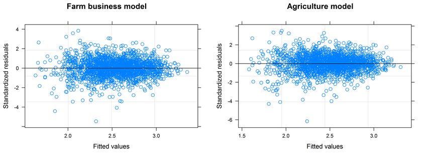
7.3 Model diagnostic plots

Figure 16. Standardised residuals plotted againsts fitted values for the farm business and agricultre
models

Figure 17. Quanitile-quantile plot for the farm business and agriculture models.

 7. References
Barnes, A., 2008. Technical Efficiency Estimates of Scottish Agriculture: A Note. Journal of
Agricultural Economics, Volume 59, p. 370–376.
Barnes, A. et al., 2010. A report on technical efficiency at the farm level 1989 to 2008,
London: Defra.
Betts, C., 2020. Characteristics of high performing grazing livestock farms in England,
London: Defra.
Crawley, M. J., 2013. The R Book. 2nd ed. Chichester: John Wiley & Sons Ltd..
Defra, 2019. Structure of the agricultural industry in England and the UK at June, London:
Department for Environment, Food & Rural Affairs.

 29

Foster, C. et al., 2007. The Environmental, Social and Economic Impacts Associated with
Liquid Milk Consumption in the UK and its Production, A Review of Literature and
Evidence, London: Defra.
Gollop, F. & Swinand, P., 2001. Total Resource Productivity. Accounting for Changing
Environmental Quality. In: C. Hulten, E. Dean & M. Harper, eds. New Developments in
Productivity Analysis. Chicago: University of Chicago Press, pp. 587-608.
Hadley, D., 2006. Patterns in technical efficiency and technical change at the farm‐level in
England and Wales, 1982–2002. Journal of Agricultural Economics. Journal of Agricultural
Economics, 57(1), pp. 81-100.
Jones, C., 2020. Characteristics of high performing cereal farms in England, London:
Defra.
Kimura, S. & Sauer, J., 2015. Dynamics of dairy farm productivity growth: Cross-country
comparison. OECD Food, Agriculture and Fisheries Papers, Volume 87.
Langton, S., 2011. Cereals Farms: Economic Performance And Links With Environmental
Performance, s.l.: Defra Agricultural Change and Environment Observatory Research
Report No. 25.
Langton, S., 2012. Grazing Livestock Farms: Economic Performance and Links With
Environmental Performance, s.l.: Defra Agricultural Change and Environment Observatory
Research Report No. 30.
Langton, S., 2013. Dairy Farms: Economic Performance And Links With Environmental
Performance, s.l.: Defra Agricultural Change and Environment Observatory Research
Report No. 31.
Pinheiro, J. et al., 2018. nlme: Linear and Nonlinear Mixed Effects Models. R package
version 3.1-137, https://CRAN.R-project.org/package=nlme, s.l.: s.n.
R Core Team, 2018. R: A language and environment for statistical computing , Vienna,
Austria. URL https://www.R-project.org/: R Foundation for Statistical Computing.
Redman, G. et al., 2018. The characteristics of high performing farms in the UK, s.l.:
AHDB.
Seufert, V. R. N. a. F. J. A., 2012. Comparing the yields of organic and conventional
agriculture. Nature, 485(229-232).
Shortall, O. & Barnes, A., 2013. Greenhouse gas emissions and the technical efficiency of
dairy farmers. Ecological Indicators, pp. 478-488.
Thirtle, C. & Holding, J., 2003. Productivity of UK agriculture: Causes and constraints,
London: Defra.
Thirtle, C. et al., 2004. Explaining the decline in UK agricultural productivity growth.
Journal of Agricultural Economics, 55(2), pp. 343-366.

 30