Characterization of Flow Rates in an In-Water Algal Harvesting Flume
←
→
Page content transcription
If your browser does not render page correctly, please read the page content below
COLLEGE OF WILLIAM AND MARY PHYSICS DEPARTMENT

Characterization of Flow Rates in an In-Water Algal
                 Harvesting Flume

                               By Kristin Rhodes
                             Advisor: Dr. William Cooke

                                       May 2012

   A report submitted in partial fulfillment of the requirements for a degree in Physics
                   from the College of William and Mary in Virginia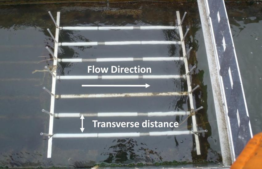
CHARACTERIZATION OF FLOW RATES IN AN IN-WATER ALGAL HARVESTING
                              FLUME

                                       KRISTIN RHODES
                               ADVISOR: DR. WILLIAM COOKE

ABSTRACT

       Algal harvesting from in-water platforms has the potential to contribute to meeting

current energy demands while simultaneously aiding in environmental remediation efforts. The

purpose of this research was to characterize the flow through an in-water algal harvesting

platform, the York River Research Platform (YRRP). The flow through the YRRP was assessed

through the use of an Aquadopp Current Profiler, which generated a current profile over a 200

hour period of deployment. In addition, a Nortek Vectrino Velocimeter was utilized to attain

instantaneous velocity measurements across the transverse distance of the platform, between

algal harvesting screens. Models of the of both the tidal height and the flow were created using

velocity readings taken during the Aquadopp’s deployment. Through power spectrum analysis

using Kolmogorov’s Laws, it was determined that the flow through the platform was congruous

with a turbulent flow model. Additionally, the change in flow between the screens was modeled

effectively with an exponential fit. From the exponential models it was determined that the

maximum flow between screens was largely independent of the overall flow outside of the

YRRP. Further research will be conducted to determine the horizontal, vertical, and transverse

flow profiles throughout the flume. The total flow as a function of the length of the platform will

also be studied in order to determine the ideal length of an algal harvesting flume of this nature.
INTRODUCTION

       Algae has the potential to be utilized as a significant resource for meeting our nation’s

liquid fuel demands, as the lipids extracted from algal cells can be converted into usable biofuels.

However, the most productive, environmentally sound, and cost-effective methods by which to

grow and harvest algae for biofuel production have yet to be determined [1]. Though many

current growth methods focus on the cultivation of a singular species, the Chesapeake Algae

Project instead uses an in-water algal harvesting flume, the York River Research Platform

(YRRP), to cultivate a robust array of wild algae while simultaneously removing excess nutrients

and carbon dioxide from the surrounding environment [2] .

       This research sought to model, measure, and characterize the flow of the water through

the YRRP. A characterization of the flow is necessary to understand the algal growth process,

and could also provide flow models for similar in-water structures. A full characterization of the

flow will also help to generate an understanding of the flow speed and flow behavior as a

function of position within the craft, and as a function of proximity to algal harvesting screens.

Ultimately this will assist in determining the ideal platform size to optimize water treatment and

algal growth. Flow characterization will also allow for the quantification of the total volume of

water treated by the flume in a given period of time. This is necessary for understanding the

flume’s effectiveness in removing excess nutrients, nitrogen, and carbon dioxide from the water,

and therefore its efficacy as an environmental remediation tool.

       The YRRP is located in the lower York River, to the East of Gloucester Point. Initially,

the YRRP contained 10 cages of 5 algal harvesting screens, each with a surface area of 1 m2 on

each side. The platform has suffered severe damage due to storms and general wear, and

consequently contained a variable number of screens throughout the research period.
An original model of the flow through the platform was generated by taking the
derivative of a sinusoidal model of the tidal cycle. The maximum value of flow recorded near
the platform was known to be 0.7 m/s, and the flow model was adjusted to fit this parameter.
The average value from the flow model was summed with the total surface area of the screens to
obtain an estimate of the total volume of water through the YRRP.
A more accurate prediction for the flow was then generated using a more sophisticated
model. The tides fall and rise in periodic motion determined by the gravitational tide-producing
forces from the moon and the sun. The model was created based on the most significant semi-
diurnal and diurnal tidal components. The most significant semi-diurnal component is the
principal lunar tidal component, which has a period of 12.42 hours, and the most significant
diurnal component is the luni-solar tidal component, which has a period of 23.93 hours [3]. The
tidal height was therefore modeled by the linear combination of two sine waves with these
periods as follows:
( ) ( ) ( ) ( )
Where:Ignoring the slight curvature of the earth and assuming a flat plane for the surface of the
water, the flow of the water was modeled as the derivative of the tidal height with respect to
time. Consequently, the flow model used was as follows:
( ) ( ) ( ( ) ( ))
where is a constant scaling factor. By generating a model of the flow, an estimate of the
expected total volume of water through the YRRP was determined.
Additionally, the characteristics of the flow at different speeds through the flume were
characterized. Turbulence occurs at higher flow speeds, and is caused by unsteady vortices of
differing sizes interact with each other, resulting in chaotic and irregular motion. In turbulent
flow, larger eddies will break up into smaller ones until the total kinetic energy is dissipated into
the internal energy of the water. Conversely, laminar flow exists when there is no disruption
between parallel layers of water, and consequently no lateral mixing or eddies occur [4].
Because wave motion is periodic, a wave field can be described as the linear combination
of different sine waves and analyzed using Fourier Analysis. A power spectral density plot can
be used to demonstrate how the power of a given wave is distributed among these sine waves.
Though the power spectrum of a measurement in a free-flowing body of water will contain
energy at all frequencies, the power spectrum identifies the frequencies at which the bulk of the
energy is concentrated [5]. Power spectrum analysis can also be utilized to determine whether
the motion of the water exhibits turbulent or laminar flow.
The rate of change of the scalar energy spectrum of a wave, E(k) can be defined as
follows:
( ) ( ) ( )where ( ) is the dissipation rate of energy from wavenumbers greater than magnitude k to
wavenumbers smaller than magnitude k.
In turbulent fluctuations, energy is supplied in length scales of order . The energy
transfer occurs in nonlinear scales until it is dissipated at scales of order .
The first part of Kolmogorov’s theory of 1941 dictates that for high Reynold’s numbers,
when turbulent motion occurs at length scales smaller than , they will be independent of the
components of motion, with no preferential spatial direction. The motion of the large
wavenumbers is at equilibrium, because the time scales at these wavenumbers are significantly
smaller than those of the eddies. Therefore:
When
( ) ( ) ( )
And ∫ ( )
Kolmogorov’s theory also stated that for high Reynold’s numbers, the turbulent motion
of small scales are purely a function of the viscosity and the energy dissipation . These two
quantities provide the Kolmogorov length and velocity as follows:
( )
( )
Consequently, the time-scale in this range can be given by:( )
Where [ ] , and [ ] .
Because [ ( )] , it follows that:
( ) ( )= ( )
At very high Reynold’s numbers, Kolmogorov’s theories dictate that the motion within
is purely a function of the scale and the energy dissipation . Consequently,
the previous equation can be rewritten as follows:
( )
( ) ( )
where is some constant.
A fit of Equation 3 was made to the velocity measurements in order to assess the
degree to which they fit to a turbulent flow model. In a purely one dimensional flow with an
incompressible fluid, the Navier-Stokes Equation is given as follows:
( ( ))
Where is the fluid density, is the flow velocity, and , and is the dynamic viscosity.
In the case of the flow through the screens, motion occurs primarily in the ẑ direction:
vz vz p 2vz
z z
Because the flow is constant along ẑ :
2
p 2 vz
z x
The x̂ component of the Navier-Stokes law gives:
p
0
x
Showing that under these conditions, constant pressure along the channel is assumed.
Now, if it is assumed that the velocity starts at zero on the wall, reaches it maximum speed half
way across the channel, and has constant curvature (so the pressure does not vary with x):
2 x W 2 x x 2v z 8v
vz v1 1 4v1 1 12
W W W
x 2
W
2v 8 v
p 2z 21
z x W
8 zv
p p0 2 1
W L
Consequently v1 can be determined by integrating to ensure that the net force on the
water is equal to the change in momentum of the water entering the flume. During a time dt ,
and amount of water hdx vz dt will leave the flume, carrying momentum hdx vz dt vz ,
while (in the absence of viscosity) an amount of water hdx v0 dt would have entered carrying
momentum hdx v0 dt v0 . The change in momentum across half of the channel is integrated,
and it must have been provided by the net force on one of the side walls:vz 4 hLv1
F hL
x x 0 W
W 2 W 2
2W2 2 hW
F
dP
dt
dx z 0
v 2
v 2
hdx v z dx v02
2
0 0 W 0
4 hLv1 W 2 x x
2
dx
2 hW
2 4v1 1 v0
W 0 W W W 2
12
hW 32v12 hW 2 8v12 hW
32v12 u 1 u du v02
2
v02 v0
2
0 60 2 15 2
This is bounded because the flow speed should not (and does not) exceed the river speed, so
4 hLv1 7v02 hW 240 L v1 Wv0
W 15 2 7 W v0
v1 Wv0 W 7 W 7
Re
v0 L 240 L 240
Wv0 0.5 m/s 0.15 m
Re 75000
106 m 2 / s
v1
75000
7 W
2200
0.15 m 33
v0 240 L 10 m
So, there will not be a parabolic transverse flow dependence unless the outside flow is
smaller (< 0.02 m/s), or if there is sufficient turbulence to make an effective (or eddy) viscosity
much larger.
When the outside flow velocity is too high, then turbulence will occur, creating an eddy
viscosity that is much higher than the normal water viscosity. The water near the algae mat will
show a boundary layer where the flow goes from 0 to v1 in a distance much smaller than W. This
means that the lines of flow will vary with z, producing a small flow component in the transverse
direction and a viscous force only in the boundary layer. We will treat the boundary layer as
having a z component of velocity that exponentially approaches the flow speed in the center of
the channel:v v1 1 e x /
MATERIALS AND METHODS
Aquadopp Profiler:
The Aquadopp Profiler utilizes the Doppler Effect to determine the current profile of a
body of water. It contains three different acoustic beams taking measurements in a variable
number of cells. It also contains internal tilt compass sensors to determine the direction of the
current, and a high-resolution pressure sensor to determine the depth.
The Aquadopp Profiler was deployed on the YRRP beginning on 12/07/11 at 10:38:35.
Velocity measurements were taken for 18 different cells at time increments of 1 minute for a
total of 200 hours.
The tidal heights are recorded by the National Oceanic and Atmospheric Administration
(NOAA) at the USCG Training Center in Yorktown, which is a short distance from the YRRP.
The average East Velocity over the first 8 cells of data for the Aquadopp measurements
was calculated. A model of the flow was determined using Equation (2), with parameters
altered in order to minimize the difference between the Model Flow and
the Measured East Velocity. Using the parameters of the Model Flow, the Model Tidal Height
was determined using Equation (1). This was plotted against the curve of the Tidal Height data
as determined by NOAA.Vectrino Velocimeter:
Measurements were made using Nortek’s Vectrino Velocimeter, a high resolution
acoustic Velocimeter using coherent Doppler processing. The Doppler Effect is the change in
pitch that occurs when the source of sound is in motion relative to the observer. The relative
change in pitch allows for quantification of the speed of the moving particle. The Vectrino
Velocimeter functions by reflecting short pairs of sound pulses off of particles in the water, and
measuring the change in frequency of the returned sound. It can therefore calculate the velocity
of such particles, which move with the overall flow of the water. The focal point of the
measurements occurs ~5cm from the transducers on the Vectrino probe.
Figure 1: The Vectrino probe. The Vectrino measures flow when the transducer sending pulses,
and the four receivers measure the Doppler Shift.
For data collection, the Vectrino was completely submerged, with the transmit axis was
positioned such that it was perpendicular to the main flow direction. A mount was constructed
for the Vectrino to enter the YRRP as depicted in Figure 2.̂
̂
̂
Figure 2: Mount for Vectrino Probe. The mount slides across cross-bar region in order to create
a transverse velocity profile. The vertical height of the mount can also be adjusted to measure
flows at varying depths.
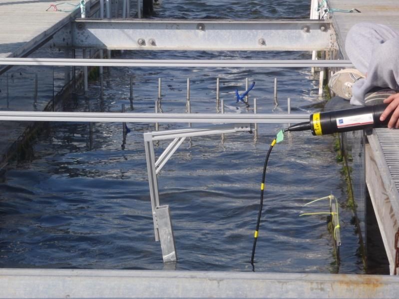
The direction of the flow between the screens is depicted in Figure 3.
Figure 3: Flow between screens in a Cage of the YRRP
Velocity measurements were made using the Vectrino Velocimeter, beginning with the
probe positioned directed against one of the screens, 13” below the surface of the water. Theprobe was then moved across the transverse distance between the screens and measurements
were made for the velocity at increments of 0.25”. Power spectrum plots were generated for the
velocity measurements, and the turbulence of the flow was assessed using a comparison of the
plot of Equation (3). An exponential fit model was generated for the flow as a function of
distance from the screens using Equation (5).
RESULTS AND DISCUSSION
Initial Flow Calculations
In initial measurements, the peak flow speed was determined to be 0.70 m/s. A flow
model with an amplitude of 0.70 was generated by taking the derivative a sinusoidal tidal model.
The rectified form of this model, used to show the absolute value of the flow velocity, is plotted
in Figure 4.
Figure 4: Projected Flow Speeds with peak flow at 0.70 m/s and an average flow speed of
0.44m/sThe average flow speed was summed with the total surface area of the screens in order to
project the total amount of water treated by the YRRP. This was determined to be 38 million
liters of water per day by the YRRP.
Aquadopp Profiler and Flow Model:
Using Equation 1, a model was created to fit the average measured Average East
Velocity from the Aquadopp readings. On account of a break in the data recordings from hours
130-153, the model was fitted to hours 11-130. A comparison of the measured East Velocity and
the Model Flow is depicted in Figure 3.
Model Flow, and Average East Velocity (Aquadopp Cells 1-8), Hours 11-130
1
0.8
0.6
0.4
Flow (m/s)
0.2
0
Average East Velocity
-0.2 0 20 40 60 80 100 120 140
Model Flow
-0.4
-0.6
-0.8
-1
Hours since 00:00:00, 12/07/11
Figure 5: Model Flow and Measured Average East Velocity from Aquadopp readings.
The Model Flow as a function of time can be given as follows:
( ) ( ) ( ( ) ( ))
The model for the Tidal Height was determined using the above parameters and Equation
1. A fit was created using the NOAA tidal height measurements, varying the value of tominimize the difference between the model and the NOAA measurements. was determined
to be 1.363 and thus the Model Tidal Height can be given as follows:
( ) ( ) ( ) ( )
The Model Tidal Height was plotted with the NOAA Tidal Height Measurements over
the time period through which the flow was modeled.
Model Tidal Height, Measured Tidal Height (NOAA USCG), Hours 11-130
3
2.5
Tidal Height (ft)
2
Measured Tidal Height
1.5
Model Tidal Height
1
0.5
0
0 50 100 150
Hours since 00:00, 12/07/11
Figure 7:Measured Tidal Height from NOAA and Model Tidal Height.
Using Equation 6, the average flow over the tidal cycle was determined to be 0.26 m/s.
This model therefore predicts that 22 million liters of water will be treated by the YRRP per day.
Vectrino Velocimeter Measurements and Power Spectrum:
Measurements were taken with the Vectrino Velocimeter on 03/15/12 during a period of
relatively high flow. Measurements were taken from directly against the screen to 9.75” away
from the screen at increments of .25”, and at a depth of 13”. Figures [8-11] depict a sampling of
Power Spectrum plots.Figure 8: Power Spectrum for velocity data taken 0.25” away from the Screen, 13” Deep. Equation 3 is plotted in red with A= 0.005. Figure 9: Power Spectrum for velocity data taken 3.25” away from the Screen, 13” Deep. Equation 3 is plotted in red with A= 0.015.
Figure 7: Power Spectrum for velocity data taken 6.5” away from the Screen, 13” Deep.
Equation 3 is plotted in red with A= 0.013.

Figure 8: Power Spectrum for velocity data taken 9.75” away from the Screen, 13” Deep.
Equation 3 is plotted in red with A= 0.015.

       The plots demonstrate that Equation 3 fits the data, corroborating the idea that a turbulent

flow exists between the screens.
Measurements were also taken with the Vectrino Velocimeter on 03/13/12 during a period of low flow. Measurements were taken from up against the screen to 7” away from the screen at increments of .25”, once again at a depth of 13”. Figures [9-11] show the Power Spectrum plots for different distances from the screens. Figure 9: Power Spectrum for velocity data taken 0” away from the Screen, 13” Deep. Equation 3 is plotted in red with A= 0.013. Figure 10: Power Spectrum for velocity data taken 3.25” away from the Screen, 13” Deep. Equation 3 equation is plotted in red with A= 0.015.
Figure 11: Power Spectrum for velocity data taken 6.5” away from the Screen, 13” Deep.
Equation 3 is plotted in red with A= 0.020.

Figure 12: Power Spectrum for velocity data taken 9.75” away from the Screen, 13” Deep.
Equation 3 is plotted in red with A= 0.030.
As depicted in the plots, the Kolomogorov model fits the power spectrum for the velocity

measurements. The slope of the spectrum plot decreases within the high frequency range, but this

can likely be accounted for by the noise of the instrument. Further data analysis is necessary to

confirm this assumption, however.

       Exponential fits were created using the transverse velocity measurements. Figure 13

shows the fit of measurements taken during a period of high flow, and Figure 14 shows a fit of

the measurements taken during low flow.

       Figure 13: Exponential Fit to velocity measurements taken during a period of High Flow
Figure 14: Exponential Fit to velocity measurements taken during a period of High Flow
The parameters of the fits for all of the different trials are shown in Table 1 as follows.
Table 1: Parameters of Exponential Fit of Transverse Velocity Plots, Fitted to Equation 4
The asymptotic velocity for the various trials is relatively constant. The average is value
7.24 cm/s with a standard deviation of 0.63 cm/s. If this is taken to be the average flow through
the platform, these models predict a treatment of 6.25 million liters of water per day by the
YRRP, which is significantly less than the original model.CONCLUSION
A flow model outside the YRRP as a function of time was determined to be ( )
( ( ) ( )), which leads to an average
flow of 0.26 m/s. If the flow outside the flume was congruous with the flow inside the flume, this
model dictates an average of 22 million liters of water being treated by the flume per day, as
compared to an initial estimate of 38 million liters. However, it was determined that the flow
inside the flume is significantly slower than the flow outside it. Exponential models were created
in order to provide a model for the transverse flow between the screens. From these models, it
was found that the average flow speed through the YRRP was 7.24 cm/s. This model predicts an
average of 6.25 million liters of later being treated by the flume per day, which is significantly
lower than expected. It was also determined that a turbulent flow exists between the screens of
the YRRP via power spectrum analysis using Kolmogorov’s theories. This has implications for
the transport of nutrients and carbon dioxide throughout the flume, as turbulent mixing plays a
significant role in the circulation throughout a water column [6].
A variety of different factors may have affected the flow cycle that were not considered
in this research. The York River estuary consists of different shoals and dunes in the riverbed in
addition to a system of channels. Scully et al. took flow measurements and found that lateral
differences in turbulent mixing are more pronounced in the channel regions and less pronounced
in the shoal regions. The greatest lateral asymmetries occur at the end of ebb tide, inducing a
shorter ebb tide over the channels, and a longer ebb tide over the shoals [6]. In the future, a
greater understanding of the waterbed’s geography could provide additional insight into the
behavior of the flow cycle.Spring tides currents lead to more mixing and less stratification of flow across the vertical
water column, while during weak tides, the stratification is more stable. Sharples et al. found that
in the York River, for the most part the water column is stratified, with short transitions to high
mixing and homogeneity along the vertical water column. Sharples et al. also determined that
the surface wind stress was equally likely to cause mixing events as Spring tides [7]. In the
future, measurements across the water column should take into account both the type of tide and
the surface winds as both can significantly affect the behavior of the flow.
This research provided new insights into the total amount of water being treated by the
York River Research Platform, in addition to creating a predictive model for the flow outside of
the flume. Future work will allow for a more in-depth quantification of the total volume of flow
through the flume in a variety of ways. First, a numerical model for the flow inside of the flume
as a function of the flow outside of the flume will be created. Horizontal and vertical profiles will
also be generated to assess variation across the platform. Ultimately, these models with be
utilized to determine the ideal length for algal harvesting structures similar to the YRRP.REFERENCES [1] McClain, J., 2010. To Harness the Wild Algae. William & Mary Ideation (http://www.wm.edu/research/ideation/science-and-technology/to-harness-the-wild- algae5832.php) [2] The Chesapeake Algae Project. William and Mary Economic Development.(http://www.wm.edu/offices/economicdevelopment/regionalprojects/chesapeak ebay/chap/index.php ) [3] Influence of Earth Tides, 2003. Geophysical Research Letters, 30. [4]Laminar & Turbulent Flows. http://udel.edu/~inamdar/EGTE215/Laminar_turbulent.pdf [5]Wave Measurements and the RDI ADCP Waves Technique. http://www.rdinstruments.com/pdfs/waves_primer.pdf [6] Scully, M.E., and C.T. Friedrichs, 2006. The Importance of Tidal and Lateral Asymmetries in Stratification to Residual Circulation in Partially Mixed Estuaries. Journal of Physical Oceanography, 37, 1496-1511. [7] Sharples, J. , J.H. Simpson, and J.M. Brubaker, 1994. Observations and Modeling of Periodic Stratification in the Upper York River Estuary, Virginia. Estuarine, Coastal, and Shelf Science, 38, 301- 312.
You can also read