Chemical Structure Elucidation from Mass Spectrometry by Matching Substructures
←
→
Page content transcription
If your browser does not render page correctly, please read the page content below
Chemical Structure Elucidation from Mass
                                                              Spectrometry by Matching Substructures
arXiv:1811.07886v1 [physics.chem-ph] 17 Nov 2018

                                                    Jing Lim1 2 , Joshua Wong∗1 , Minn Xuan Wong∗1 , Lee Han Eric Tan1 , Hai Leong Chieu1 , Davin
                                                                                     Choo3 , Neng Kai Nigel Neo4
                                                   1
                                                       DSO National Laboratories, Singapore, 2 Department of Computer Science, Stanford University,
                                                             3
                                                               ETH, Zurich, 4 Department of Chemistry, National University of Singapore
                                                             jinglim2@stanford.edu, {wjialain,wminnxua,tleehan,chaileon}@dso.org.sg,
                                                                                  chood@ethz.ch, nnnk@u.nus.edu

                                                                                                  Abstract
                                                              Chemical structure elucidation is a serious bottleneck in analytical chemistry
                                                              today. We address the problem of identifying an unknown chemical threat given
                                                              its mass spectrum and its chemical formula, a task which might take well trained
                                                              chemists several days to complete. Given a chemical formula, there could be over a
                                                              million possible candidate structures. We take a data driven approach to rank these
                                                              structures by using neural networks to predict the presence of substructures given
                                                              the mass spectrum, and matching these substructures to the candidate structures.
                                                              Empirically, we evaluate our approach on a data set of chemical agents built for
                                                              unknown chemical threat identification. We show that our substructure classifiers
                                                              can attain over 90% micro F1-score, and we can find the correct structure among
                                                              the top 20 candidates in 88% and 71% of test cases for two compound classes.

                                                   1       Introduction
                                                   The identification of unknown chemical compounds remains one of the major challenges for an-
                                                   alytical chemistry. Continuous improvements to instrumental capabilities have allowed a much
                                                   bigger number of compounds to be separated and detected even at low concentrations. As a result,
                                                   many new compounds in environmental or biological matrices can now be found in a short time,
                                                   rendering chemical structure elucidation (CSE) a serious bottleneck in the analysis workflow. This has
                                                   resulted in a greater emphasis in computer-aided CSE for fast and accurate identification of unknown
                                                   compounds. State-of-the-art commercial software built to assist CSE requires user interaction with
                                                   an analyst, or additional chemical post filtering processes such as boiling point, retention index and
                                                   partitioning coefficient [15, 16].
                                                   In this paper, we apply CSE to identify chemical agents controlled by the Chemical Weapons
                                                   Convention [5]. The use of structurally information-rich techniques such as nuclear magnetic
                                                   resonance (NMR) require high sample purity and relatively high concentrations, and when these are
                                                   not available, chemists could only obtain the mass spectrum and its chemical formula through the
                                                   use of various gas chromatography detectors [16]. A mass spectrum is a plot of the ion signal as
                                                   a function of the mass-to-charge ratio, reflecting the relative abundance of detected ions. Usually
                                                   the first strategy in CSE is to match the spectrum against a library of known spectra. For unknown
                                                   compounds, a manual or software assisted interpretation of the mass spectra must be performed. This
                                                   task is non trivial and might take a well trained chemist a few days, as a mass-to-charge ratio value
                                                   (m/z) with only integer precision can represent an immense number of theoretically possible ion
                                                       1
                                                       Indicates equal contributions. This work was conducted when Jing Lim served as a research intern in DSO
                                                   National Laboratories.

                                                   2nd NIPS Workshop on Machine Learning for Molecules and Materials (MLMM 2018), Montréal, Canada.
(b) Molecular structure
(a) Mass spectrum
Figure 1: We show the mass spectrum and the corresponding molecular structure of dimethyl
methylphosphonate (C3 H9 O3 P ). This example is drawn from the NIST Chemistry Webbook [1].
structures. We show an example of a mass spectrum and it’s corresponding chemical structure in
Figure 1. Given the mass spectrum (e.g., Figure 1(a)) and the chemical formula (e.g., C3 H9 O3 P .),
the objective of CSE is to pin down the chemical structure of the compound (e.g., Figure 1(b)).
Software such as MOLGEN [8] could enumerate all possible structures given a chemical formula, but
the number of possible structures could be in the millions. Previous work attempted to incorporate
different substructure classifiers and filtering mechanisms, but the workflow always involve a chemist
in the process to fine-tune substructure selection [8, 15, 16]. In this paper, we propose to address this
problem in a completely automated workflow, presenting a list of ranked candidates as outputs for
identification. We experimented on two compound classes in a data set provided by the Organisation
for the Prohibition of Chemical Weapons (OPCW). Our approach ranked the provided ground truth
structure in the top 20 positions in 88% and 71% of test cases for two different compound classes.
If our approach can narrow down the list of candidates to 20 or less, we could then apply more
computationally intensive computer simulation of fragmentation of these candidates for a final
identification.
2 Related Work
One notable early work on computer-aided CSE from mass spectrometry (MS) is [19]. They applied
principal component analysis, latent discriminant analysis and neural networks with one hidden
layer to substructure classification. Empirically they analyzed 4 cases studies, manually selecting
substructure classifiers, and used predicted substructures to assist analysts to reduce the number of
candidates. These substructure classifiers were incorporated into the MOLGEN-MS [8] software.
In [8], they mentioned that the substructure classifiers “typically require a user interaction for a
critical check of classification results and adding additional structural information”. More recently,
Schymanski, Meinert, Meringer, and Brack [15, 16] combined MOLGEN-MS with additional
substructure information from the NIST database [10] as well as a number of post-filtering criteria
such as boiling point, retention index and partitioning coefficient. Out of 71 test cases, they found
that the MOLGEN-MS and NIST classifiers can reduce the number of candidates to below 100 in
70% of the cases. With the post-filtering criteria, they further reduce the number to 93% below 100
and 70% below 10. In the use of substructure classifiers in MOLGEN-MS, Schymanski, Meringer,
and Brack [16] have cautioned that the trial and error approach is required to select the substructure
classifier and a chemist’s judgement is needed to manually review the classifier list prior to candidate
generation to ensure that they do not restrict the candidate generation in undesired ways which could
potentially prevent a fast identification.
Together with the burgeoning use of high-resolution, high-accuracy MS and tandem MS, alternative
identification strategies have arisen that involve the use of online compound database (PubChem [2]
and Chemspider [13]) searching. These have spurred multiple analytical companies such as Thermo
Fisher, Agilent Technologies, Waters and ACD Labs to develop commercial software, such as Mass
Frontier (Thermo Fisher), Masshunter Profinder (Agilent), Progenesis Q1 (Waters) and ACD/MS
Workbook Suite (ACD Labs), that make use of these online databases to yield substructure information
based on the mass spectrum of the unknown compound. With this information, the chemist can
then postulate probable structures on which the software would perform an in-silico fragmentation
2Figure 2: The workflow for computing a score f (c|{M S, CF }) of a candidate structure, c, given a
mass spectrum and its chemical formula, {M S, CF }.
and from the fragments generated, a match value to the experimental mass spectrum is calculated.
However, not only is there a limited amount of spectral databases available for high-resolution and
tandem mass spectrometry, the requirement of a well trained chemist to elucidate the unknown
structure does not make the structural elucidation process any less of a challenge.
In this work, we propose to automate the entire process from substructure selection to candidate
ranking. Previous work [19] used the ToSim [17] software to search for substructures in compounds
to generate the ground truth for training substructure classifiers. In this work, we compile training
data for substructure classification by checking if substructures are subgraphs of the chemical
compound structures. Now, substructures responsible for certain m/z in a mass spectra may not be
subgraphs due to rearrangement reactions. On the other hand, the ground truth for the actual spectral
fragments responsible for m/z spikes in a mass spectrum are unavailable unless we employ software
such as Mass Frontier, an expensive operation if we have to run it through all candidates during
testing. Hence, we trained our substructure classifiers based on ground truth established through
subgraph isomorphism (SGI). As a result, the substructure classifiers learn to predict the presence
of substructures as subgraphs, rather than as actual spectral fragments. Empirically, we show that
the substructure classifiers can achieve high micro F1-scores, and in our analysis, we illustrate with
examples of substructures which may not coincide with spectral fragments, but are still useful in the
CSE process.
3 Substructure Matching for CSE
We propose to elucidate the chemical structure of a compound given its mass spectrum and chemical
formula. To rank candidate structures generated by MOLGEN, we build a scoring function that
scores candidate structures against a given (M S, CF ) pair. We evaluate our results by the rank of the
correct structure among the candidates. We illustrate the workflow for building the scoring function in
Figure 2. Given a training data set of (M S, CF ) pairs mapped to their underlying molecular structure
S ∗ , we first gather a set of substructures from the training data, and run an automated substructure
selection algorithm to select a small number of useful substructures (box (a) in Figure 2). We then
use machine learning to learn classifiers to predict the presence of the selected substructures given
each (M S, CF ) pair (box b). During testing, we use these classifiers to compute the likelihood of
each substructure given a (M S, CF ) pair. Given postulated candidate structures, we score each
candidate by comparing predicted substructures against the candidate structure (box (c)). We describe
the components in more detail in the remaining of this section.
33.1 Substructure selection
From the training data of structures, we propose to first enumerate possible interesting substructures
as candidate substructures for further selection. We tried the two approaches for enumerating possible
substructures in a given structure. The first approach is a simple rule-based cleaving of bonds, and
the second rely on a commercial software called Mass Frontier.
Three-stage fragmentation (3SF) The first approach is an iterative cleaving of bonds to obtain
possible substructures: given structures in the training data, we gather the substructures resulting
from cleaving any one edge, and perform this same cleaving action to each substructure recursively
two more times. The resulting substructures are counted, and we only keep those which occur within
one standard deviation from the mean, discarding those that are either too common or too rare.
Mass Frontier (MF) For the second approach, we apply Mass Frontier from Thermo Fisher Scien-
tific to generate stable substructures given a structure. We initialised MF through its fragmentation
settings to generate fragments from molecules under electron impact ionisation. We also limit the
number of reaction steps for fragment generation, ensuring that most of the fragments present in the
spectrum are captured, but not unnecessarily extend the amount of computing time needed. Similar
to the previous substructure selection method, we only keep fragments whose occurrences are within
one standard deviation from the mean.
Decision Tree Selection Denote the set of substructures (gathered by either MF or 3SF) as CS.
In this section, we propose to select a small subset of CS to be used for matching, for reasons of
computational efficiency. Since the purpose of the substructures is to help find the correct structure
among all candidates generated by MOLGEN, we aim to select a subset of CS that can help
discriminate between candidates generated by MOLGEN. We take 1 to 3 representatives from the
training data set and run them through MOLGEN to generate all possible candidate structures. We
denote the set of generated structures as the set C. For each candidate c ∈ C, we run SGI to determine
if each substructure s ∈ CS is a subgraph of c, forming the vector v(c) = {δ(s ∈ c)}s∈CS , where
δ(s ∈ c) is 1 if s is a subgraph of c, and 0 otherwise. We define the equivalence relation c1 ∼ c2 if
and only if v(c1 ) = v(c2 ). Two equivalent candidates contain exactly the same substructures in CS
as subgraphs.
The equivalence classes define the resolution power of the set CS: two equivalent candidates would
not be distinguishable by matching substructures in CS. On the other hand, not all substructures in
CS are necessary to divide C into these equivalence classes. We aim to select a minimal subset of CS
that is sufficient in dividing the candidates into these equivalence classes. We achieve this by running
the decision tree classifier [3] in scikit-learn [12] by using the structures as instances, substructures
as features, and equivalence classes as target labels. We collect all substructures with non-zero
Gini-importance into CS ∗ , as our minimal subset of distinguishing substructures for matching.
In our experiments, for computation efficiency, we only used candidates generated from 1 to 3
representatives for each compound class from the training data. Note that CS ∗ has the same
resolution power as CS on the candidates used for selecting substructures, i.e. it divides CS into the
same equivalence classes. In our experiments, the MF approach of generating substructures resulted
in around 100,000 unique substructures in CS, while CS ∗ only contains around 1,000 substructures.
3.2 Neural Network Classifier
In this section, we describe the neural network classifier used to predict the presence of substructures
given (M S, CF ) pairs. The objective of the substructure classifier is to learn to predict the presence
of a substructure in a compound, given clues from the mass spectrum. However, establishing the
actual spectral fragments responsible for the spikes in the mass spectrum is too expensive during
testing for matching candidates. Hence, we decided to train substructure classifiers to predict if a
substructure is a subgraph of the structure that generates the mass spectrum.
Initial experiments with classifiers such as support vector machines [4] performed mediocrely for the
final ranking evaluation. Hence, we built a one dimensional convolutional neural network (CNN)
on the mass spectrum for feature learning, illustrated in Figure 3. For an input (M S, CF ) pair, we
L2-normalise M S and represent CF as counts of chemical elements existing in the compound. We
4Figure 3: Neural network architecture for predicting substructures.
extract features from M S using a two-layered convolutional neural network. The first convolution
layer consists of filters of sizes 3, 4, 5, 6, and 7, with 100 filters for each sizes. The second convolution
layer consists of filter sizes 2, 3, and 4, also with 100 filters for each size, resulting in a total of 150,000
filters. CF is concatenated to the flattened outputs of the second CNN layer before classifying the
input using two fully connected (FC) layers. The number of dense units in each layer follows that
of the number of output classes. Between each FC layer, there is a dropout layer with dropout rate
of 0.25. The Rectified Linear Unit (ReLU) is used as activation functions except for the output
layer which uses the sigmoid function. The output are the probabilities {p(s|{M F, CF })}s∈CS ∗ of
the substructures being present in the chemical compound given {M S, CF }. We train the neural
networks for all selected substructures in a multi-task manner, where all the neural networks share
all layers except the final layer. We train the network for 100 epochs using Adam optimizer and
minimise the binary cross entropy.
3.3 Subgraph Isomorphism
Subgraph isomorphism (SGI) is NP-complete [6]. As we use a large number of SGI computations, it
is the main bottleneck in our workflow. To improve efficiency, we leverage the fact that, for a fixed
compound, we compute SGI for a large number of similar graph and subgraph pairs.
For any two graphs Gi and Gj such that Gi is a subgraph of Gj (notation-
ally Gi ⊆ Gj ), certain necessary conditions must hold. By contrapositive,
if any of these conditions fail, then we can quickly deduce that Gi is not
a subgraph of Gj . One such condition is the “set of atoms”. For example,
for H2 0 to be a subgraph of Gj , Gj must contain at least 2 hydrogen
atoms and 1 oxygen atom. For each graph and subgraph, we compute the
following signatures: ATOMS refers to all atoms that appear in the graph, Figure 4: Sarin’s graph.
and NEIGHBOURS is a list of the list of neighbours for each type of atom. Image from NIST Chem-
As each substructure and candidate structure are involved in many SGI istry WebBook [1].
pair evaluation, the pre-processing time for graph signature computation
is negligible compared to the actual time spent in SGI evaluations.
We illustrate the above-mentioned signatures with the Sarin compound C4 H10 F O2 P (See figure 4).
We represent nodes by their atom string and edges by the number of bonds.
• ATOMS(Sarin) = {C, C, C, C, F, O, O, P }
• NEIGHBOURS(Sarin) = {N br[C], N br[F ], N br[O]N br[P ]}, where
– N br[C] = {{C}, {C}, {P }, {C, C, O}}
– N br[F ] = {{P }}
– N br[O] = {{C, P }, {P, P }}
– N br[P ] = {{C, O, O, O, F }}
By comparing graph signatures, we only run the SGI implementation in igraph [6] in cases where the
signatures are insufficient in ruling out SGI.
5Figure 5: Neural network architecture of compound class classifier.
3.4 Final scoring and ranking
The final score of a candidate structure C given a mass spectrum M S, and chemical formula, CF , is
Y
f (c|{M S, CF }) = (p(s|{M S, CF }) · δ(s ∈ c) + (1 − p(s|{M S, CF })) · δ(s ∈/ c)) , (1)
s∈CS ∗
where CS ∗ is the set of substructures selected by the decision tree algorithm in Section 3.1, and
p(s|{M S, CF }) is output probability of the substructure neural network classifier. This is computed
for all candidate structures generated by MOLGEN. We then rank the candidates in descending order
of their scores f (c). Note that the p(s|{M S, CF }) in Equation 1 only depend on the M S and not
the candidate c, and so candidate structures which are in the same equivalence classes (i.e., contain
exactly the same substructures in CS ∗ ) would have identical scores, and hence will be ranked equally.
Also note that δ(s ∈ c) is defined to be 1 if s is a subgraph of c, and 0 otherwise. We decided to use
SGI instead of checking if s is a spectral fragment for c, as this check is expensive, and hence we
have also trained the classifiers on ground truth established via SGI.
4 Experimental Results
We conducted experiments on the Validation Group Working Database (VGWD) 2017 provided by
the Organisation for the Prohibition of Chemical Weapons (OPCW) [11]. The database provided
the chemical table files of all chemicals in the database as well as their corresponding spectra files.
Using the index file given by OPCW, the organophosphorus compounds in the database were split
into 29 compound classes according to their functional group. Due to the time needed to prepare and
select the substructures for the training data, we decided to apply the workflow on each compound
class separately, and we selected two compound classes for experimentation: Phosphonate (PPN),
the biggest compound class with 1715 instances, and Phosphonothionate (PPTN), the fourth in size
with 293 instances, for our experiments. To show that the approach is general and not constrained
by this limitation, we built a classifier that can classify organophosphorus compounds into the
correct compound class that could serve as a pre-processing step. We conducted the compound class
classification experiments on 27 of the 29 classes which contain more than 10 instances. We show
that we can obtain extremely high accuracies of over 99% for this problem (see Section 4.1)
4.1 Compound Class Classification
We did a five-fold cross validation on the data set to classify compound classes into these 27 classes.
The data set consists of a total of 4223 instances, with 12 in the smallest class and 1715 in the biggest
class. This task seems a lot easier than the substructure classification task: simply training a support
vector classifier [4] with default parameters gives an accuracy of 98.5% with a linear kernel, 84.4%
with a polynomial kernel, and 84.8% with a rbf kernel. We also tried with a neural network classifier
similar to the one used for substructure classification, as shown in Figure 5. Features are extracted
from the L2-normalized M S using three one-dimensional convolution layers with filter sizes 3 and 4.
The number of filters for each progressive layer are 64, 128 and 256. Between each convolution layer,
max pooling is implemented with pool size and stride 2, to provide spatial invariance to overcome
minor shifts in mass spectra peaks due to isotopes. Features are extracted from the CF using two fully
connected layers with 32 and 64 units respectively. Extracted features are flattened and concatenated
and used as input to two fully connected layers with 128 units in each layer. Between the fully
connected layers are dropout layers with dropout rate of 0.25. ReLU is used as activation function
6Class Id # Cand Name
PPTN 1 848 O-sec-butyl o-propyl ethylphosphonothionate
2 17758 O-propyl o-trimethylsilyl isopropylphosphonothionate
PPN 1 2092 3-methylbutyl propyl ethylphosphonate
2 48872 Pinacolyl trimethylsilyl methylphosphonate
3 45522 Propyl 2-diethylaminoethyl methylphosphonate
Table 1: Representatives used in the substructure selection with decision trees for each compound
class. The #Cand column shows the number of structures generated by MOLGEN given the chemical
formula.
except the output layer where the softmax function is used instead. The network was trained for 100
epochs and batch size of 32 using Adam optimizer and minimize the categorical cross entropy. We
adopted the idea of smooth labelling commonly used in Generative Adversarial Networks [14] during
training to reduce the extremity of confidence probability. We also trained with class weights (derived
from the training data) to overcome class imbalance. We achieved 99.5% accuracy with this neural
network architecture.
4.2 Data Preparation
The OPCW VGWD 2017 database [11] provides the chemical table files of all chemicals in the
database as well as their corresponding spectra files, the latter being generated under electron impact
condition. In order to obtain CS, the complete set of substructures, by the Mass Frontier approach, we
run the Mass Frontier fragmentation on the whole training set, taking about 3 minutes per compound,
and generating around 100,000 unique substructures. We experimented on PPTN (with 293 instances)
and PPN (with 1715 instances) compound classes, with random 5:1 train-test split ratio resulting
in1430/285 and 244/49 compounds for the two classes respectively. In the substructure selection
process with decision tree described in Section 3.1, we used MOLGEN to generate candidates for
representatives for each compound class. These representatives are chosen based on the different
functional groups that each compound class would possess. We list the representatives selected for
our experiments in Table 1. In our experiments, we compare our results using different number of
representatives for substructure selection.
We use MOLGEN to generate candidate structures for ranking during evaluation. However, MOLGEN
can take very long to generate all candidates, and it will only produce any output at all at the end of
its execution. For efficiency, we configured MOLGEN to stop at 1 million candidates. MOLGEN can
also be configured to generate only candidates that agree with specified annotations, which reduces
the number of candidates generated. We conducted two sets of experiments as follows:
ADDGT We run MOLGEN without annotation. In cases where there are more than 1 million
candidates and the ground truth structure is not among the 1 million candidates, we add the
ground truth into the list of candidates. In this experiment, we compare the performance of
the two substructure generation approaches, 3SF and MF. We also assume that compound
class classification is performed perfectly in this setting.
STRICT We constrain MOLGEN with annotations to the phosphorus (valency = 5, hydrogen bonds
= 0, double bond = 1), sulfur (double bonds = 1) and oxygen (double bonds = 1) atoms,
depending on the compound class (PPN or PPTN), so that only valid candidates of the
class are generated. For the family PPTN, MOLGEN failed to generate the ground truth in
two instances (because we stopped the generation at 1 million), but for PPN, MOLGEN
failed in 41 instances. In these cases, we count these test instance as failures. Cases wrongly
classified in compound class classification are also counted as failures.
4.3 Results
In this section, we report results using the neural networks described in Section 3.2. To compare 3SF
and MF substructure generation methods, we evaluate them in the ADDGT settings and show the
results in Table 2. We see that the MF approach does slightly better than 3SF for ranking the ground
7Class (#cases) SG #REP #SSTR #CAND Time Top 5 Top 20
PPN (285) 3SF 1 1,131 641,032 259min 82.1% 88.8%
MF 1 663 641,032 214min 81.8% 88.8%
PPTN (49) 3SF 1 577 327,908 32min 77.6% 89.8%
MF 1 393 327,908 27min 83.7% 89.8%
Table 2: Results in the ADDGT setting. The columns denote the method of substructure generation
(SG), the number of representatives (#REP) used for selecting substructures, the average number of
candidates (#CAND) and time taken for each instance, and the percentage of instances with ground
truth ranked in the top 5 or 20 instances. The average time is based on running each test case on 4
parallel threads.
Class (#cases) #REP #SSTR #CAND Top 5 Top 20 #G20 Micro-F1
PPN(285) 1 397 291,319 43.5% 54.4% 36.5% 91.5%
2 885 291,319 53.7% 63.9% 26.7% 92.6%
3 1550 291,319 62.8% 70.9% 20.4% 91.2%
PPTN (49) 1 160 84,424 73.5% 81.6% 4.1% 91.9%
2 343 84,424 77.6% 87.8% 2.0% 92.7%
Table 3: Results in the STRICT setting. The columns denote the number of representatives (#REP)
used for selecting substructures, the average number of candidates (#CAND), the percentage of
instances with ground truth ranked in the top 5 or 20 instances, the percentage of instances where the
group (of candidates with equal scores) containing the ground truth has a size bigger than 20, and the
micro-F1 of the substructure classifiers.
truth in the top 5 positions. The MF approach would produce more chemically viable substructures as
it is based on chemical principles. However, the results we achieved with 3SF is only slightly worse,
especially for the larger class PPN.
For the STRICT settings, we only experiment with the MF substructure generation approach. As
shown in Table 3, our approach could still rank more than 80% of cases in the top 20 for the smaller
compound class of PPTN, but only 70.9% for PPN when 3 representatives were used to generate
candidates for substructure selection. In Table 3, we see that the micro-F1 for both PPN and PPTN
are similar. The reason for the worse performance in PPN is due to the fact that substructure selection
with 1 to 3 representatives does not provide enough substructures, and resulted in large equivalence
classes of candidates with equal scores. When this happens, we take the worst ranking of the group
containing the ground truth as the rank of the ground truth. Performance improves as we increase the
number of representatives used for substructure selection, resulting in more substructures used for
discriminating between candidates. In the column #G20, we show the percentage of instances with
more than 20 structures in the equivalence class (of structures with equal scores) of the ground truth:
these are cases where the approach fails automatically to rank the candidate in the top 20. We see that
the majority of mistakes made (e.g., 45.6%, 36.1% and 29.1% for PPN for 1, 2 and 3 representatives)
are due to the fact that the group of the ground truth contains more than 20 candidates (E.g., 36.5%,
26.7% and 20.4% respectively).
We also experimented with support vector machines [4] in scikit-learn [12] with worse results. For
example, for SVM with linear kernel, we could only achieve 69.4% for PPTN with 2 representatives,
compared to 87.8% with neural networks.
We show the average run times for ranking the candidates generated by MOLGEN in Table 2, where
the run time is computed by running 4 parallel threads on each candidate, on a Intel(R) Xeon(R) CPU
E5-2620 v4 at 2.10GHz. This timing, however, does not include the time MOLGEN takes to generate
candidates. In most cases, MOLGEN can finish generating all candidates in less than 1 hour.
8(a) 0.9997 (b) 0.9819 (c) 0.1589 (d) 0.0011
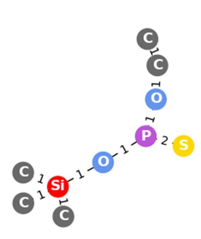
Figure 6: Example fragments with their predicted scores for O,O-dipropyl methylphosphonothionate,
with the probability of the prediction that they are present in the structure given the mass spectrum.
(b) 0.9985
(a) 0.9993
Figure 7: Example fragments with their predicted scores for O-isopropyl O-trimethylsilyl isopropy-
lphosphonothionate, with the probability of the prediction that they are present in the structure given
the mass spectrum in the two representative setting.
4.4 Analysis and Discussion
In order to better understand this prediction model, we take a look at the predicted substructures for
some of the test cases. As mentioned in Section 2, the substructures used mat not be actual spectral
fragments. Herein, we would take a look at 2 test cases, O,O-dipropyl methylphosphonothionate and
O-isopropyl O-trimethylsilyl isopropylphosphonothionate, to understand the factors that affects the
prediction accuracy. Looking at the PPTN results under the STRICT setting with 1 representative, the
test case O,O-dipropyl methylphosphonothionate has the ground truth ranked as the most probable
compound when its spectrum was analyzed. Substructures with –OCCC and –PC moieties were
predicted as present (Figures 6(a) and 6(b)) while those with longer alkoxy and alkyl chains were
predicted as absent (Figures 6(c) and 6(d)). This example showed that the machine learning is able to
predict with high accuracy, the presence of fragments with the correct moieties.
As we compare the PPTN results under the STRICT setting that made use of both 1 and 2 repre-
sentatives, the test case O-isopropyl O-trimethylsilyl isopropylphosphonothionate has the ground
truth ranked 3842nd and 8th positions respectively. While the STRICT setting with 1 representative
used a dialkyl alkylphosphonothionate, the STRICT setting with 2 representatives used both a dialkyl
alkylphosphonothionate and silylated alkyl alkylphosphonothionate. The addition of a silylated
representative resulted in Si-containing differentiating fragments in the second setting. As we take a
look at the fragments, the trimethylsilyl moiety (Figure 7) is indeed predicted with high confidence
to be present in the test case and this resulted in a huge improvement in the ground truth ranking.
Therefore, we should choose representatives to contain the different functional groups that the model
would be trained to recognise.
5 Conclusion
In this paper, we proposed to automate the chemical elucidation process to produce a ranked list of
structures given the mass spectrum and chemical formula of a compound. We conducted experiments
within compound classes in the OPCW VGWD database. Since our experiments showed we could
classify instances into compound classes accurately (see Section 4.1), this does not compromise the
applicability of our approach. We experimented with two compound classes of chemical agents from
the OPCW VGWD database, and showed that we can rank the correct structure in the top 20 positions
9in over 88% of the test cases for the PPTN compound class, and over 71% for the PPN class. The
computational time taken to rank the candidates of one test case is usually under one hour. If the
correct structure is ranked within the top 5 or 20 candidates, the chemist can verify these structures
experimentally or by computational mass spectral simulation to confirm the correct structure. In
future work, we would like to investigate structure generation approaches such as [7, 9, 18] to
bypass MOLGEN in this workflow. We believe that this automated workflow would be important in
improving the efficiency of the work of analytical chemists.
Acknowledgements
We would like to thank Kian Ming Adam Chai, Hoe Chee Chua and Lee Hwi Ang for useful
discussions.
References
[1] National institute of standards and technology chemistry webbook. https://webbook.nist.
gov. Accessed: 2018-08-02.
[2] E. E. Bolton, Y. Wang, P. A. Thiessen, and S. H. Bryant. PubChem: integrated platform of small
molecules and biological activities. In Annual reports in computational chemistry, volume 4,
pages 217–241. Elsevier, 2008.
[3] L. Breiman. Classification and regression trees. Routledge, 2017.
[4] C.-C. Chang and C.-J. Lin. Libsvm: a library for support vector machines. ACM transactions
on intelligent systems and technology (TIST), 2(3):27, 2011.
[5] B. Clinton. Chemical weapons convention. US Department nf State Dispatch, 4:849–851, 1993.
[6] G. Csardi and T. Nepusz. The igraph software package for complex network research. Inter-
Journal, Complex Systems, 1695(5):1–9, 2006.
[7] W. Jin, R. Barzilay, and T. Jaakkola. Junction tree variational autoencoder for molecular graph
generation. In J. Dy and A. Krause, editors, Proceedings of the 35th International Conference on
Machine Learning, volume 80 of Proceedings of Machine Learning Research, pages 2323–2332,
Stockholmsmässan, Stockholm Sweden, 10–15 Jul 2018. PMLR.
[8] A. Kerber, R. Laue, M. Meringer, and K. Varmuza. MOLGEN-MS: Evaluation of low resolution
electron impact mass spectra with ms classification and exhaustive structure generation. Adv
Mass Spectrom, 15(939-940):22, 2001.
[9] Y. Li, O. Vinyals, C. Dyer, R. Pascanu, and P. Battaglia. Learning deep generative models of
graphs. CoRR, abs/1803.03324, 2018.
[10] National Institute of Standards and Technology. Mass spectral library (NIST/EPA/NIH), 2005.
[11] Organisation for the Prohibition of Chemical Weapons, The Hague, The Netherlands. Validation
Group Working Database (VGWD), version: VGWD_2017, 2017.
[12] F. Pedregosa, G. Varoquaux, A. Gramfort, V. Michel, B. Thirion, O. Grisel, M. Blondel,
P. Prettenhofer, R. Weiss, V. Dubourg, et al. Scikit-learn: Machine learning in python. Journal
of machine learning research, 12(Oct):2825–2830, 2011.
[13] H. E. Pence and A. Williams. ChemSpider: an online chemical information resource, 2010.
[14] T. Salimans, I. Goodfellow, W. Zaremba, V. Cheung, A. Radford, and X. Chen. Improved
techniques for training gans. In Advances in Neural Information Processing Systems, pages
2234–2242, 2016.
[15] E. Schymanski, C. Meinert, M. Meringer, and W. Brack. The use of ms classifiers and structure
generation to assist in the identification of unknowns in effect-directed analysis. Analytica
chimica acta, 615(2):136–147, 2008.
[16] E. L. Schymanski, M. Meringer, and W. Brack. Automated strategies to identify compounds on
the basis of GC/EI-MS and calculated properties. Analytical Chemistry, 83(3):903–912, 2011.
[17] H. Scsibrany and K. Varmuza. Tosim: Pc-software for the investigation of topological similari-
ties in molecules. Software Development in Chemistry, 8:235–249, 1994.
[18] M. Simonovsky and N. Komodakis. Graphvae: Towards generation of small graphs using
variational autoencoders. CoRR, abs/1802.03480, 2018.
[19] K. Varmuza and W. Werther. Mass spectral classifiers for supporting systematic structure
elucidation. Journal of Chemical Information and Computer Sciences, 36(2):323–333, 1996.
10You can also read