Climate Policy in an Unequal World: Assessing the Cost of Risk on Vulnerable Households
←
→
Page content transcription
If your browser does not render page correctly, please read the page content below
Munich Personal RePEc Archive

Climate Policy in an Unequal World:
Assessing the Cost of Risk on Vulnerable
Households

Malafry, Laurence and Soares Brinca, Pedro

Potsdam Institute for Climate Impact Research, Nova School of
Business and Economics

5 May 2020

Online at https://mpra.ub.uni-muenchen.de/100201/
MPRA Paper No. 100201, posted 10 May 2020 12:17 UTC
Climate Policy in an Unequal World: Assessing the Cost of
              Risk on Vulnerable Households*
                           Laurence Malafry†‡                Pedro Soares Brinca§
                                 PIK                             Nova SBE

                                                    Abstract
          Policy makers concerned with setting optimal values for carbon instruments to address
      climate change externalities often employ integrated assessment models (IAMs). While these
      models differ on their assumptions of climate damage impacts, discounting and technology,
      they conform on their assumption of complete markets and a representative household. In the
      face of global inequality and significant vulnerability of asset poor households, we relax the
      complete markets assumption and introduce a realistic degree of global household inequality.
      A simple experiment of introducing a range of global carbon taxes shows a household’s
      position on the global wealth distribution predicts the identity of their most-preferred carbon
      price. Specifically, poor agents prefer strong public action against climate change to mitigate
      the risk for which they are implicitly more vulnerable. This preference exists even without
      progressive redistribution of the revenue. We find the carbon tax partially fills the role of
      insurance, reducing the volatility of future welfare. It is this role that drives the wedge between
      rich and poor households’ policy preferences, where rich households’ preferences closely
      mimic the representative agent. Estimates of the optimal carbon tax and the welfare gains of
      mitigation strategies may be underestimated if this channel is not taken into account.

      Keywords: Climate change, Inequality, Risk, Optimal carbon policy
      JEL Classification: H23, H31, Q54, Q58

   * We thank Per Krusell, John Hassler, Conny Olovsson, Kjetil Storesletten, Ann-Sofie Kolm, Martin Ljunge, Hans
Holter, Rob Hart, Jo João Duarte, Miguel H. Ferreira. We also thank seminar participants at IIES and Department of
Economics at Stockholm University, PIK, NOVA SBE, ISEG, Lisbon Macro Workshop, CEF.UP, U Católica Lisbon. This
work was supported by the German Federal Ministry of Education and Research (BMBF) under the research projects
SLICE (FKZ: 01LA1829A) and CLIC (FKZ: 01LA1817C). Pedro Brinca is grateful for funding provided by Fundação para
a Ciência e a Tecnologia (UID/ECO/00124/2019, UIDB/00124/2020 and Social Sciences DataLab, PINFRA/22209/2016),
POR Lisboa and POR Norte (Social Sciences DataLab, PINFRA/22209/2016) and CEECIND/02747/2018.
   † Potsdam Institute for Climate Impact Research, Telegraphenberg A56 14473 Potsdam, Germany
   ‡ Corresponding author: malafry@pik-potsdam.de
   § Nova School of Business and Economics, Universidade NOVA de Lisboa, Campus de Carcavelos, 2775-405

Carcavelos, Portugal
1 Introduction
To date, models of climate and the economy have calculated optimal carbon policy under the
assumption of complete markets and a representative agent. A growing empirical literature
on climate impacts highlights the distributional costs of climate change, with the global poor
being particularly vulnerable. In order to explore the implications of relaxing these assumptions
from the integrated assessment modelling literature, we introduce a standard incomplete mar-
kets framework. Thus, in addition to an uncertain global climate state, households also face
idiosyncratic productivity shocks for which they can not insure away. Calibrating the model to the
global economy, we find that there are significant differences in the cost of carbon faced across the
wealth distribution driven implicitly by individual vulnerability. Poor households are vulnerable
to future shocks, due to their relative paucity in private insurance. Hence, poor households prefer
ex ante stronger public action through high carbon taxation, even in the absence of progressive
redistribution. However, the direction and predictability of future transfers are of primary concern
in the identity of a household’s most preferred carbon policy. In this setting, the public insurance
co-benefit yields large welfare gains for vulnerable households.
The International Panel on Climate Change (IPCC) details the impact (both realized and
potential) on the world’s more vulnerable population, in its chapter on Livelihoods and Poverty
in the 2014 Climate Change Report1 . In this chapter the report discusses the interaction of
climate change and the challenges faced by the poor and economically vulnerable. While climate
change implies specific threats related to shifting weather patterns, increased incidence of natural
disasters, decreased land arability, etc., the report also notes that climate change exacerbates
existing vulnerabilities experienced by the poor. While there will be regional heterogeneity
in climate change, the impact will be felt globally: the poor in all regions will suffer from
market disruption, declining agricultural yields, reduced access to water, etc. Indeed, while poor
households in low income countries (LICs) will incur the greatest costs of climate change impacts,
the IPCC notes that inhabitants of some middle income countries (MICs), including urban Chinese,
are among the most at risk to climate-related impacts.
One popular tool for policy makers is the integrated assessment model (IAM)2 , which aims
to capture the features of the climate change problem, including: modelling the carbon system;
atmospheric carbon’s relationship to global temperature; temperature’s relationship to welfare
1 SeeOlsson et al. (2014)
2 e.g.Dynamic Integrated Climate-Economy model DICE, Nordhaus and Sztorc (2013); Climate Framework for
Uncertainty, Negotiation and Distribution, FUND, Tol (1997), and Golosov et al. (2014)
1loss; and the economic system, including modelling the micro-foundations of savings and fossil
fuel use. There are a wide range of IAMs, which differ on the assumptions they make; however,
a common feature of these models is their reliance on a representative agent assumption for
assessing consumer behaviour and welfare impacts. While there has been a trend towards
providing regional detail, the unit of analysis remains nation states or regional blocs3 . In this
paper, we change the unit of analysis to individual households that experience varying degrees of
vulnerability in the face of their economic decisions and the threat of climate change.
Climate change impacts are likely to vary significantly across the population, depending
on household characteristics, including: location, occupation, wealth, etc. This paper focuses
primarily on wealth inequality. It looks to address the question of how a realistic distribution of
household wealth changes the optimal carbon taxation problem, from the familiar representative
agent framework. It seeks to answer both how and how much inequality matters for optimal
carbon taxation. The primary channel we investigate is the cost that risk imposes across the
population, and the role carbon taxation can play as public insurance. When capital markets are
incomplete, households need to take precautionary action to insure against idiosyncratic shocks.
Moving assets to the future then becomes a question of consumption smoothing, aggregate risk
mitigation4 , and insurance against idiosyncratic shocks. It is this last component that is absent
from the current body of literature on optimal carbon taxation.
Models with incomplete markets and heterogeneous households have become common in more
traditional research areas of macroeconomics, allowing a better understanding of distributional
impacts and implications of public policy. These types of models offer insights into the role of
public policy as a way of mitigating risks through, for example, social security and progressive
taxation (see Heathcote et al. (2009) for an introduction). Climate policy can play a similar role.
In light of poor households’ explicit vulnerability to climate change, relaxing the representative
agent assumption seems a natural progression for IAMs, used for assessing the welfare impacts of
climate change, and delivering estimates for the optimal policy response. In general, aggregation
will miss the nuances of household behaviour and welfare implications across the distribution.
Currently there is little in the literature that explicitly models how climate change variously affects
different people, especially through climate risk and individual uncertainty.
In order to explore these implications, we present a simple integrated assessment model that
3 e.g.RICE Nordhaus and Yang (1996), WITCH Bosetti et al. (2006), and REMIND Leimbach et al. (2010)
4 See Gerst et al. (2010) and Howarth et al. (2014) for examples of how aggregate risk impacts the social cost of
carbon and policy decisions with regards to climate change mitigation.
2encompasses the carbon, climate and economic systems. The model is calibrated to match: a
global CO2 emissions path scenario from the IPCC, aggregate risk and damage estimates from
the IAM literature, and moments from the global distribution of income and wealth. The model
includes both aggregate climate risk and idiosyncratic household productivity shocks, which
may be correlated. The primary exercise is to evaluate a range of global carbon taxes, observe
household welfare responses, and identify their most preferred policy.
This policy preference depends on both the characteristics of the household and the policy.
The carbon tax is determined in advance of the period in which it applies; thus, household
welfare is considered ex ante. In order to isolate the impact of wealth inequality on the identity
of a household’s most-preferred tax, we initially suppress the revenue redistribution channel
and equalize idiosyncratic risk-profiles. In this analysis, households differ only on their wealth
endowment; a determinant of their ability to self-insure. Clearly, ex post redistribution of the tax
revenue can be a significant contributor to the distribution of welfare impacts. However, thorough
analysis of revenue recycling, double-dividends, and interaction with other distortionary taxation
is beyond the scope of this study.
Our first finding is that when idiosyncratic risk is correlated with aggregate risk, such that the
variance of a household’s future labour income increases in a bad aggregate state, the dispersion
of the population’s tax preference becomes large and quantitatively relevant. This result arises
from the way an increase in the risk on labour earnings affects households along the distribution
of wealth. Increasing the carbon tax decreases earnings volatility and allows households to reduce
their costly precautionary savings. This effect is larger for households who receive a relatively
large proportion of their earnings from labour - i.e. the poor.
Our second finding is that the economic vulnerability of poor households in the standard
incomplete markets framework creates a role for carbon taxation as a form of public insurance
that can substitute for private savings. Carbon taxation reduces the impact of extreme climate
realizations on earnings. However, quantitatively, the direction of transfers inherent in the carbon
tax rebate is the most important factor in a household’s policy preference arising from climate-
related damages. In addition, the predictability of these future transfers is also of key concern.
For today’s wealthiest households, if the future carbon tax rebate is sufficiently uncertain, they
would rather no public intervention in climate change at all.
In comparison to the more familiar setting of complete insurance markets and a representative
agent, the optimal carbon tax under such assumptions resembles the preference of only the most
3wealthy households in the experiments allowing for household inequality. This implies that
introducing risk and inequality can substantially change the calculus of optimal carbon taxation,
and also that the direction and predictability of carbon revenue redistribution should be of first
order consideration to policy makers.
2 Background
A growing empirical literature on the impacts of climate change identifies significant distributional
considerations. As mentioned above, the IPCC notes that the global poor will be especially
susceptible to decreasing agricultural yields, access to clean drinking water, and global market
disruption. Skoufias (2012) summarizes some of the quantitative evidence on the welfare impacts
of climate change, particularly with respect to global poverty. The author notes that there are
sectoral considerations, particularly with respect to decreasing agricultural productivity. However,
the most vulnerable population may be urban wage-labourers, who are particularly exposed to
food price shocks. The global demographic shift towards urbanization also implies that this could
be a key driver on climate change’s influence on poverty metrics. Dell et al. (2013) review the
empirical literature on weather shocks and climate impacts. Several of the channels through which
weather can impact welfare include: labour productivity, health and mortality, and industrial and
services output. While not addressing household inequality directly, the authors do note that
climate impacts are likely heterogeneous, with damage being higher for low income countries.
On longer horizons, climate-induced health shocks can create linked generational issues. Weather
shocks, which create better conditions for disease vectors or decrease maternal and infant nutrition,
can have effects on infant mortality as well as long-run implications for adult outcomes (e.g.
education, wealth, health and mortality).
2.1 Related literature
Recent work related to this topic has looked at environmental taxes in the context of distributional
issues for public finance. Fremstad and Paul (2019) examine carbon taxation in an input-output
model of the US and look at the impacts of on a range of socio-economic characteristics while,
Bosetti and Maffezzoli (2013) and Fried et al. (2018) use an incomplete markets framework and
examine the distributional impacts of various carbon taxation schemes. None of these studies
present an IAM, or indeed an externality, the aim not being to derive an optimal tax, but rather to
explore the implications of a potentially regressive environmental tax policy and the potential for
4double dividends through various revenue recycling schemes. In contrast we hold constant the
fiscal structure of the global economy, and only allow climate specific taxation to vary.
This paper is also closely related to the work done on expanding IAMs to account for
heterogeneity of impacts. Models with regional heterogeneity, such as RICE and FUND, account
for geographical heterogeneity, and can be used to make assessments of the distributional impacts
of climate change on poverty-related metrics, as in Skoufias (2012). Anthoff et al. (2009a) use an
IAM framework with diminishing marginal utility and equity weighting to discuss and quantify
the implications of global income inequality across many regions. To our knowledge, however, no
study has relaxed the representative agent assumption in an IAM framework, and thus welfare
analysis relies on aggregates, such as the elasticity of a poverty count to changes in GDP.
A recent study, Dennig et al. (2015) acknowledging the need to move beyond regional ag-
gregation, explores an alternative to the standard RICE framework by incorporating income
inequality within regions. In the likely case that damages are greater for the poor within a region,
the authors find that the optimal carbon tax would be well in excess of the case which does
not account for intra-regional income inequality. While similar in spirit our work differs from
this in several key ways: we focus on individual household behaviour in the face of incomplete
insurance markets, rather than representative agents of regional income quintiles. We do not
currently explore regional climate damage heterogeneity, or formulate an explicitly regressive
climate damage. And in our framework, the savings decision for each household is endogenous
to the climate policy rather than a fixed proportion of income, which ends up being a key channel
through which inequality drives policy impacts. Finally, our analysis focuses on ex ante impacts
caused by un-insurable risk. Therefore, our contribution is from the perspective of today’s poor,
rather than ex post analysis of the impact on the future poor.
3 The Framework
In order to address the question on how optimal carbon policy setting responds to changes in
household wealth inequality, we propose the following simple dynamic framework, which adopts
much of the structure from Golosov et al. (2014). The model is a dynamic stochastic general
equilibrium model, which includes a simple description of climate change mechanics and allows
for heterogeneous households. Thus it features a dynamic decision on household consumption
and savings, including a precautionary motive for individual risk. Competitive firms use fossil
energy as an input in production that increases the stock of greenhouse gases (GHGs) in the
5atmosphere, which accumulate over time and increase global mean temperature. The increase in
temperature has a negative impact on aggregate production. Finally, there exists an aggregate
shock related to the climate change externality, such that today’s decision makers don’t know the
severity of the future temperature increase.
While the framework is dynamic, the time horizon is finite and for the purposes of this exercise
we limit the number of periods to two. Working with household inequality and aggregate risk is
challenging, and especially so in a climate change framework, where households without perfect
foresight need to form expectations about the evolution of the atmospheric carbon stock as well as
the aggregate stock of capital. This limited time horizon is sufficient for exploring the implications
of income and climate risk across the distribution of households, and we conjecture that the
findings of the two period model will carry over to longer horizons.
3.1 Households
Each household i chooses a sequence of consumption, ci,t and savings, k i,t+1 to maximise their
expected lifetime utility taking aggregate prices, wt and, rt , as given. It solves:
T
max
ci,t ,k i,t+1
∑ βt−1 IE[u(ci,t )] (1)
t =1
s.t. ci,t + k i,t+1 = (1 + rt − δ)k i,t + wt li,t hi,t + gi,t
k i,t+1 ≥ −b
where the households supply their period t labour endowment, li,t , (normalized to 1) inelastically.
As in Bewley-Aiyagari-Hugget-type models, hi,t is an idiosyncratic labour productivity state that
modifies an agent’s labour income through the effective supply. Agents also have different wealth
holdings, where k0 is an initial endowment. Markets are incomplete, and households cannot
borrow beyond the constraint b. Households may also receive a government transfer, gi,t , financed
by the revenue from carbon taxation. Aggregate consumption, labour and capital supply are given
by summing individual household contributions.
n n n
Ct = ∑ ci,t Lt = ∑ li,t hi,t Kt = ∑ ki,t . (2)
i =1 i =1 i =1
63.2 Production
The product market is competitive, where representative firms solve a static problem each period
by choosing how much capital, Kt , labour, Lt , and fossil energy, Et , to use in order to maximize
profits.
max (1 − D (St )) F̃ (Kt , Lt , Et ) − rt Kt − wt Lt − (κ + τt ) Et , (3)
Kt ,Lt ,Et
where F (˜.) is production before damages are subtracted and F (Kt , Lt , Et , St ) = (1 − D (St )) F̃ (Kt , Lt , Et ).
Fossil energy can be produced at constant marginal cost, κ, and is in large enough supply such
that there are no scarcity rents. While scarcity is a feature of oil and gas fuels, coal is in virtual
infinite supply from the perspective of the intended model horizon. As firms are small they do
not recognize the contribution of their own emissions to climate change. However, a regulator can
implement a tax, τt , in order to impact their energy use. The climate externality manifests itself in
the form of a reduction in aggregate production, 1 − D (St ), where ”damage”, D (St ) is increasing
in the atmospheric stock of carbon, St . In the model, carbon decreases production for a given set
of inputs.
3.3 Climate change
The Greenhouse Effect arises from the growing stock of atmospheric carbon, St . As the stock of
carbon grows, the energy flow out of the earth’s atmosphere decreases and results in rising global
temperatures. Economic activity contributes to the stock of carbon through the combustion of
hydrocarbon energy, Et . While there is a potential to model the complexity of the climate system,
including multiple carbon reservoirs, feedback effects, etc., we employ a more concise statement
of the climate system. The details of this system are outlined in the appendix.
As mentioned earlier, damage takes the form of a reduction in aggregate output. This is a
large simplification of the negative impacts that a rising global mean temperature would have on
human welfare. One could imagine other ways in which climate damage could be represented,
such as direct loss to household utility, or an increase in the capital depreciation rate, however
many IAMs, including Nordhaus’ DICE model, assume a loss of aggregate output. For the sake
of comparison to popular formulations of other IAMs, we choose to follow this assumption and
implement the aggregate damage function proposed in Golosov et al. (2014).
71 − D (St ) = exp(−θk,t St ) (4)
Climate change damage is also a source of aggregate risk, where the eventual realization of
atmospheric carbon’s potency as a GHG is a source of uncertainty faced by decision makers in the
model. For simplicity, we assume there are two possible realizations of the aggregate shock, θk ,
which occurs in the future. θhigh occurs with the probability of πhigh and denotes a high impact
the climate externality, while θlow occurs with probability 1 − πhigh .
4 Representative agent reference case
The solution to the model framework when markets are complete is equivalent to solving the
model in the absence of income risk and borrowing constraints. If, in addition, global households
are represented by an agent with mean wealth, the optimal tax has the familiar interpretation of
the Pigouvian tax, which is set in order to equate the marginal private cost to the marginal social
cost (in the case of a negative externality). With the ability to aggregate all agents in an economy
to a single representative agent, it is also easy to define a social welfare function to be optimized:
to maximize the representative agent’s utility. Thus, we turn to the planning solution to identify
the optimal level of emissions (which implies the optimal tax value) under complete markets.
T
max
Ct ,Kt+1 ,Et
∑ βt−1 IE[u(Ct )]
t =0
s.t. Ct + Kt+1 = F (Kt , Lt , Et , St ) − κEt (5)
This problem delivers the first order condition
T
u′ ( ct+s )
FE − κ = IEt ∑ β s −1 FS (Kt+s , Lt+s , Et+s , St+s )St′ +s , (6)
s =1
u′ (ct )
where primes denote a function’s first derivative with respect to Et . The right hand side of
this expression is often referred to as the social cost of carbon (SCC) and includes the damage
associated with the negative externality from fossil fuel use, both in the current period and future
8periods through the persistence of the carbon pollutant. A regulator can implement the planning
solution by setting the carbon tax equal to the SCC,which is equal to the difference between the
marginal private benefit of fuel use (marginal product of energy FE ) and the marginal private cost,
κ, at the social optimum fuel allocation5 . The carbon revenue is rebated as a lump sum to the
representative household.
5 Stylized model and calibration
In order to understand how household inequality may impact the setting of an optimal carbon
policy, we propose a stylized version and calibration strategy of the dynamic model summarized
above. The stylized model retains the features that are important for exploring the channels
through which inequality and climate vulnerability matter. Dynamics coupled with uncertainty
provide the channel through which the current poor are implicitly more vulnerable to climate risk.
5.1 Period 1 as an endowment economy
As an illustrative simplification from the Section 2 framework, we assume that there is no
production in the first period, but rather households can consume and save from their initial
endowment. Household inequality stems from the initial distribution of assets. An implication
of there being no production is that there is no fossil fuel use in period 1, and thus the stock of
carbon is only impacted endogenously by firms use of fuel in period 2. Production in period 2
yields factor prices from which households earn income in period 2.
This stylized model is summarized by the following household and firm problems, and their
resulting equilibrium conditions.
max u(ci,1 ) + βIE[u(ci,2 )] (7)
ci,1 ,ci,2
s.t. ci,1 + k i,2 = ωi
ci,2 = (1 + r2 − δ)k i,2 + w2 hi,2 + gi,2
k i,2 ≥ −b
where ωi is household i’s initial endowment.
5 See Golosov et al. (2014)
9The resulting optimal savings condition for household i is given by:
− u′ (c1,i ) + βIE[ R2 u′ (c2,i )] + µi = 0 (8)
µi [k2,i + (−b)] = 0
µi ≥ 0
Assuming CRRA utility, an unconstrained household i will save according to:
(w2 hi,2 + R2 k2,i + gi,2 )σ
σ
(ω − k2,i ) = IE (9)
βR2
Assuming Cobb-Douglas production, period 2 factor prices and firm input demands are given by
the solution to the firms problem as stated in the previous section:
rt = αe−θt,k St Ktα−1 L1t −α−ν Etν (10)
wt = (1 − α − ν)e−θt,k St Ktα Lt−α−ν Etν (11)
κ (1 + τt ) = νe−θt,k St Ktα L1t −α−ν Etν−1 (12)
From this we can see that fossil fuel demand is decreasing in τ , and thus can be set by the
regulator to internalize the climate change externality. Also factor earnings are decreasing in the
atmospheric stock of carbon.
5.2 Generating inequality
Household inequality in the stylized model arises from two sources: a random wealth endowment
that places the recipient on the global wealth distribution; and an idiosyncratic labour productivity
draw that adds to the initial endowment resources in the first period, as well determining the
potential for future earnings. These sources of idiosyncratic uncertainty are potentially correlated,
in that a household with a higher wealth endowment may be more likely to experience a high
labour productivity shock in period 2. Labour is supplied inelastically, so a household’s period
2 labour income is dependent on their period 2 productivity realization, and the prevailing
aggregate wage.
Under this structure, the distribution of wealth is controlled by choosing a distribution for
the initial wealth endowment. Income inequality consists of multiple states, which are meant
10to represent a household’s position on the global income distribution. In general, there can be
many income states, in order to meet more precise income inequality targets. Clearly, a realistic
representation of global income inequality would require many income states - especially to
represent the difference between those in poverty in the developing world and those living in
poverty in a wealthy nation.
5.3 Calibrating the stylized model
In order to give the stylized model a quantitative grounding, we proceed by calibrating the model
to reflect the global interaction of climate and the economy over two periods of fifty years each.
The model has three broad categories for calibration: preferences and technology, carbon and
climate, and household inequality.
Preferences and technology
We adopt fairly standard assumptions for preferences and technology from the macroeconomics
literature, including CRRA utility, Cobb-Douglas production, and full depreciation. In the short-
run, the degree of substitutability between capital-labour and energy should be relatively limited.
However, the length of periods in the model allow assumptions that correspond to longer horizon
characteristics of the production side. Factor shares, α and ν, are based on averages from historic
data, with respective values 0.3 and 0.04 taken from Golosov et al. (2014). The final parameter on
the firm side is the constant marginal cost of fossil fuel use, κ, which we calibrate endogenously
to achieve the business-as-usual atmospheric stock of carbon estimates from the most recent IPCC
report.
The choice of β is an important and controversial one in IAMs, as it determines the weight
that current decision makers put on future generations, when the bulk of climate change is due
to occur. The value of the optimal policy is very sensitive to the selection of this parameter (see
e.g. Tol (2009), Saelen et al. (2008) and Anthoff et al. (2009b) for discussion). However, in the
absence of heterogeneity across households in regards to β, it is not essential for understanding
the question of intra-generational inequality.6 For now we choose 0.98 as an annual rate, which is
in a standard range for this parameter in the family of IAMs.
6 It
is perhaps worth discussing the role of heterogeneity in time preference as a theory of inequality and a means
of generating realistic distributions of wealth in equilibrium (see for example Krusell and Smith (1998)) Clearly if
households have varying preferences for future outcomes, this opens up another dimension for setting a one-size-fits-all
carbon policy. We leave this to be explored in further work.
11Carbon and climate
The carbon system specification of Golosov et al. (2014) requires three parameters that govern the
response of the carbon stock over time, ϕ L , ϕ0 , and ϕ. We set ϕ L = 0.2 to reflect the fact that 20%
of an emissions pulse will remain in the atmosphere forever. Likewise, ϕ governs the gradual
decay of the portion of carbon in the atmosphere that is subject to natural absorption processes.
Set to match the observation that this excess carbon has a half life of 300 years, (1 − ϕ)300/50 = 0.5,
this yields a value of about 0.109. Finally, ϕ0 is identified by observing that roughly half of a given
flow of emissions are removed from the atmosphere after 30 years. Thus ϕ0 = 0.4 satisfies the
following expression from equation 16: 1 − 0.5 = 0.2 + 0.8ϕ0 (1 − 0.11)3/5 .
S2 is the atmospheric carbon stock associated with IPCC predictions for business as usual
(laissez faire equilibrium) 4◦ C increase in temperature by 2100. We can find this by using a
formula from Arrhenius (1896), which relates an increase in the stock of carbon over pre-industrial
levels to global mean temperature.7
ln SS0 S
ln 600
4 = ∆T = λ =3 (13)
ln 2 ln 2
where λ denotes the sensitivity of temperature to atmospheric carbon concentration (or more pre-
cisely denotes the increase in temperature resulting from a doubling of pre-industrial atmospheric
carbon concentration, which is here set to 3◦ C). This corresponds to an atmospheric carbon stock
value of 1,500 gigatonnes of carbon (GtC). This is roughly 900 GtC in excess of pre-industrial
levels. Thus 900 GtC becomes the calibration target for the business-as-usual (BAU) value of S2
(after normalizing S0 to 0). To find out how much carbon is emitted in the second period alone,
we return to the IPCC BAU scenario which predicts roughly 2◦ C warming by 2050, and using
the same method implies S1 = 350 GtC. Taking the difference between the two periods’ stocks
900−350
implies that our laissez-faire economy has to produce φE2 = S2 − S1 , E2 = 0.49 ≈ 1100GtC.
The exponential functional form that climate damage takes requires the calibration of θ,
which can be found by solving the relationship 1 − D (S) = exp(−θS2 ). Following the calibration
of Golosov et al. (2014), who also include uncertainty in their estimates, we choose {θh , θl } =
{2.046 · 10−4 , 1.060 · 10−5 }. These values imply a loss to aggregate output of roughly 20% and 1%
respectively, if S2 reaches 900 GtC by 2100. Assigning probabilities to the two states, again we
7 See Hassler et al. (2016) for further information.
12follow the Golosov et al. (2014) calibration {πh , πl } = {0.068, 0.934}.
Household inequality
The final category for calibration is household inequality. As explained above, there are two
sources of household heterogeneity, which arise from two sources of economic inequality. Agents
in the model are assigned an initial wealth and labour productivity profile. Initial household
wealth is distributed according to the wealth distribution in Davies et al. (2011). According to this
study the level of wealth in our base year 2000 is 44,000 per adult (PPP), and the distribution is
summarized below in 1.
Decile 1 2 3 4 5 6 7 8 9 10 Gini
World wealth share % 0.1 0.3 0.6 1.1 1.6 2.4 3.8 6.3 13.1 70.7 0.802
Table 1: Distribution of Wealth
Agents are also assigned a productivity state in the first period, which corresponds to their
position in the income distribution. There are five productivity states calibrated according to the
quintiles of the global income distribution (PPP) in Ortiz and Cummins (2011) and shown in the
calibration Table 2 on page 14. we assume that whatever causes a household to be productive
also causes them to be wealthy, such that the initial wealth endowment is distributed according to
a household’s position on the income distribution (and vice versa). Since the first period is an
endowment economy, a household’s first period productivity state determines two things: their
belief about their future earnings (through the probability transition matrix) and the total size of
their period 1 endowment. Thus, each household receives two endowments, one that represents
their initial wealth holdings, and one that represents the labour income they earn during the first
50-year period. As income is a flow, we calculate the income endowment by taking the level of
income (PPP) in the base year, and grow it at the growth rate of world GDP over the first period
and then sum all years. We then take this total amount and divide it in proportion to a quintile’s
share of total income. Each member within a quintile receives an equal amount of that quintile’s
share.
6 Carbon tax experiment
As an exercise to examine the impact of a carbon tax over the distribution of households, we
evaluate the stylized model over a grid of tax values, and examine the response of households
13Parameter Value Description Source
Preferences
β 0.98 Annual discount factors Macro literature
σ 1.5 Co-efficient or relative risk aversion Author choice
Technology
α 0.3 Capital’s value share of output Macro literature
ν 0.04 Fossil energy’s value share of out- (Golosov et al., 2014)
put
δ 1 Full capital depreciation Author choice
b 0 Household borrowing limit Author choice
Carbon and climate
θl 1.9341 · 10−5 Climate damage elasticity in low (Golosov et al., 2014)
state
θh 2.3780 · 10−4 Climate damage elasticity in high —”—
state
[πl , πh ] [0.932, 0.068] Probabilities of aggregate states —”—
ϕ L , ϕ0 , ϕ 0.2, 0.4, 0.109 carbon depreciation rates
Inequality
Income quin- [0.827, 0.117, 0.023, Share of global income Ortiz and Cummins (2011)
tiles 0.019, 0.014]
Table 2: Parameters Calibrated Exogenously
across the wealth distribution, the idea being that the characteristics of an individual household
will lead to varying welfare impacts, and thus a most-preferred tax value. As the first period is
an endowment economy, the carbon tax is only levied in the second period when production
occurs. However the value of the tax is ”negotiated” in the first period. Although pessimistic, it is
perhaps not an unrealistic assumption that a globally coordinated tax needs to be set in advance
of the period in which it becomes active. Choosing the carbon policy in advance implies that
welfare analysis is from the perspective of period 1. Thus a household’s favourite tax is chosen ex
ante according to its beliefs about what will happen in the future.
Given the degree of inequality in the world, there is substantial opportunity to increase welfare
through redistribution strategies, or pursuing ”double dividend” tax relief. In the absence of
distortionary taxes in the model, we opt for lump sum redistribution of the carbon tax revenue.
There are many possible ways to share the tax revenue, and this will have a large impact on the
identity of an agent’s most preferred tax. For this exercise, we explore several approaches for
handling the tax revenue. In the first case, we discard the tax revenue in order to isolate the
mechanisms associated with the carbon tax’s impact on capital and labour income. Discarding
revenue is clearly suboptimal; however, it reveals a few channels through which the carbon tax
can influence a household’s welfare and thus most preferred policy (and the implied carbon
concentration).
The second approach is to rebate the tax according to two different rules, uniform and
14regressive. The response of a household’s policy preference to the way in which revenue is
rebated highlights the importance of redistribution and risk mitigation in the face of incomplete
insurance markets. Clearly a uniform redistribution rule is a very progressive use of the carbon
tax revenue, and the range of most preferred taxes reflects this. The regressive rule rebates the
revenue in proportion to a household’s second period productivity realization. Thus a high
income realization in the second period also means a high carbon rebate.
Another key assumption in the incomplete markets framework is the persistence of the income
process. If the income process is serially correlated, then a household’s current position gives
information about their future income as well. While there is likely income persistence across
generations, especially on the global income distribution, we use an i.i.d income process for the
starting point in my analysis. Thus a household’s current income productivity does not carry
any information about tomorrow’s productivity realization, and a household’s policy preference
depends only upon its cash on hand in period 1. In addition to i.i.d income processes, we will
explore the implications of income persistence later in this section.
All welfare impacts are calculated as conditional welfare changes and measured in consumption-
equivalent variation. Welfare impacts are conditional on agent characteristics included in the
model, i.e. wealth, k and labour productivity, h.8 λi (k, h) solves the following equation, and is
interpreted as the change in consumption across all states and periods that leaves household i,
with wealth k and productivity h, indifferent between the unregulated equilibrium and living
through the equilibrium induced by the policy change.
2 2
∑ βt−1 IE[u((1 + λi (k, h))ci,t∗ )] = ∑ βt−1 IE[u(c̃i,t )] (14)
t =1 t =1
∗ } is household i’s sequence of consumption under the equilibrium without mitigation
where {ci,t
and {c̃i,t } is household i’s consumption sequence under a given climate policy.
6.1 Discarded revenue
We begin with an experiment where the carbon tax revenue is discarded. Following the calibration
described above reveals that a standard calibration of climate damage is insufficient to make any
agent better off. Figure 1 shows the difference between gross output and output net of carbon
tax revenue. From the gross output curve, we see that the carbon tax increases the availability of
8 See Floden (2001) for discussion.
15aggregate resources over a range of the instrument. The difference between the two curves is the
revenue raised by the regulator from levying the carbon tax on fossil fuel use.
Figure 1: Output response to carbon tax
At the baseline calibration for climate sensitivity, carbon taxation is welfare decreasing for
all agent types, if the revenue is discarded. In order to proceed, we make an adjustment to the
damage parametrization, which will become a point of comparison for both the case where tax
revenue is discarded, as well as the cases where revenue is returned. The extent of damage from
climate change is one of the most uncertain aspects of calibration in IAMs. If the climate is more
sensitive than the standard calibration, then temperature will rise more quickly, and damage will
be more severe. In an alternative high climate sensitivity calibration, we assume that damage to
production is twice as bad in expectation as in the previous calibration. Here 10% of production
will be lost when atmospheric carbon reaches 1500 GtC by 2100, rather than 5%. To do this we
leave the elasticity of damage in the high damage state unchanged at θh = 1.9341 ∗ 10−5 , but
increase the elasticity of damage in the low state to θl = 6.0335 ∗ 10−5 . The high and low aggregate
state probabilities remain unchanged. The big implication of increasing the elasticity of damage
is that the benefits from reducing emissions outweigh the costs, even when the tax revenue is
discarded. This is a way of understanding how the carbon tax affects households in the absence
of redistribution. Taking the carbon tax rebate out of the policy means that household welfare can
only be influenced through the tax’s impact on labour and capital earnings.
The first case for this experiment is one where the state of the climate does not have implications
for the idiosyncratic risk. That is, the pay-offs and transition probabilities in the idiosyncratic
states are the same whether the aggregate state is good or bad. In addition there is no income
16persistence across periods, as agents face i.i.d probability. Thus an agent in period 1 is equally
likely of transitioning to one of the five income states in period 2. While perhaps unrealistic in a
global inequality context, an i.i.d probability transition matrix is attractive for my initial analysis,
as it ensures that households have identical income risk profiles. Thus households differ only on
the amount of resources available to them in the endowment period. We leave the assessment
of persistent income states for sensitivity analysis. Figure 2 reveals that there is little difference
between household preferences for carbon taxation. Since income earned over 50 periods is much
larger than initial wealth, total cash on hand reflects a household’s position in the initial income
quintiles.
High climate sensitivity
0.12
0.1
0.08
τ
0.06
0.04
0.02
0
0 1000 2000 3000 4000
Cash on hand
Figure 2: HH Wealth Endowment vs Most Preferred Carbon Tax - no rebate
Note: This figure shows the relationship between household cash on hand in the initial period and its policy preference for the following period.
In this scenario, the following assumptions hold: the government discards the tax revenue; the climate is more sensitive than under the standard
assumptions; and income risk is not correlated with aggregate climate risk. The pattern of household policy preference shows very little dispersion
by wealth.
The reason for this result comes from the symmetry in how the sources of household earnings
are impacted by climate change damage in the model. With full depreciation and Cobb-Douglas
production, the proportional change in the factor earnings are quantitatively very similar in this
case.9 This symmetry means that households who receive their earnings entirely from labour, or
entirely from capital, benefit from the carbon tax similarly.
If, on the other hand, household idiosyncratic risk is positively correlated with the aggregate
climate state, this symmetry between earnings sources breaks down. Following the notion that
climate impacts will be unequally distributed across the population, we explore the implications of
9 In addition, if utility was logarithmic there would be no savings adjustment at all by households, even in the case
below where we assume idiosyncratic risk is positively correlated with aggregate climate risk.
17adverse shocks hitting a subset of the population; the idea being that low productivity households
will be impacted more by climate change than high productivity households. Some examples of
how this might occur is from the evidence of temperature on labour productivity. Dell et al. (2012)
discuss the existing empirical evidence noting that sectors which involve outdoor labour, such as
agriculture, mining, construction, forestry, etc. see drops in productivity during high temperature
weather. Agriculture is arguably the most susceptible to climate change impacts, and the global
agricultural labour force is largely concentrated in low income countries and amongst low earners.
From the equity premium literature Mankiw (1986) shows that when asset markets are
incomplete, the concentration of ex post adverse shocks can increase the ex ante value of existing
market assets. This logic translates into the climate change framework when idiosyncratic
productivity is correlated with the aggregate climate state. To explore this we introduce a mean-
preserving spread to the idiosyncratic productivity states, when the aggregate climate state is bad.
Thus, the volatility of labour productivity increases when climate damage is most severe. Since all
households are equally likely to be subject to these shocks in the future, it does not change their
expected labour income, only its volatility. Their labour productivity states are thus:
h1 − µ h2 − µ h3 − µ h4 + µ h5 + 2µ (15)
where µ is a parameter that makes the productivity worse for the three lowest quintiles, but
doesn’t alter the expected value of tomorrow’s income productivity realization. In this case,
the uncertainty of labour income increases putting additional pressure on poor constrained
households who rely completely on their future productivity realization for period 2 welfare. We
choose a µ equal to 0.01, which under my income state calibration results in a roughly 70% loss
in productivity for the lowest quintile should the climate realization be the high damage state.
From an aggregate perspective this may seem like a high number. However, recent studies on
disaggregated impacts, such as Krusell and Smith Jr (2015), find damage impacts similar to these
magnitudes even in scenarios which correspond to aggregate global damages that are in line
with the low damage aggregate state. Figure 3 reveals a relationship between a household’s most
preferred tax and its wealth endowment.
18High climate sensitivity
0.12 Inequality
Rep Agent
0.1
0.08
τ
0.06
0.04
0.02
0
0 1000 2000 3000 4000
Cash on hand
Figure 3: HH Wealth Endowment vs Most Preferred Carbon Tax - no rebate, correlated risk
Note: This figure shows the relationship between household cash on hand in the initial period and its policy preference for the following period.
In this scenario, the following assumptions hold: the government discards the tax revenue; the climate is more sensitive than under the standard
assumptions; and income risk is correlated with aggregate climate risk. The pattern of household policy preference now shows significant dispersion
by wealth. The representative agent comparison for this experiment is included, where insurance markets are complete (no idiosyncratic income
risk), and all households have mean wealth.
Poor constrained households prefer a tax more than twice as large as their wealthier uncon-
strained counterparts. This result arises from constrained households having greater exposure
to climate risk. Agents who rely entirely upon labour income benefit from stronger action on
climate change, as cutting emissions reduces losses associated with the worst potential outcomes.
Agents with private savings will not be hurt as badly in these realizations, as they will have
additional resources on hand for adaptation regardless of their labour productivity state. Amongst
unconstrained households the relative composition of earnings determines their most preferred
tax, with the fourth income quintile still receiving a large enough proportion of their earnings
from labour to prefer a higher carbon tax than the wealthier quintile above them.
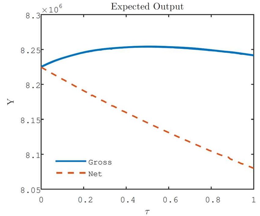
There are, however, additional general equilibrium considerations for wealthy household tax
preference. Figure 4 charts household tax preference against their wealth endowment, when only
considering the portion of their earnings from capital. This reveals a reversal of the pattern under
total earnings. Here wealthier households prefer a higher tax. The reason for this is that carbon
taxation reduces savings more quickly amongst poorer households. This reduction in savings
benefits wealthier households through higher returns on their own savings, which they are not
inclined to adjust as quickly in the face of increased carbon taxation.
19Expected utility maximizing tax - capital earnings only
0.045
0.04
0.035
0.03
τ 0.025
0.02
0.015
0.01
0.005
0
0 1000 2000 3000 4000
Cash on hand in period 1
Figure 4: HH Wealth Endowment vs Most Preferred Carbon Tax - capital earnings only
Note: This figure shows the relationship between household cash on hand in the initial period and its policy preference for the following period
when only taking into account capital earnings. In this scenario, the following assumptions hold: the government discards the tax revenue; the
climate is more sensitive than under the standard assumptions; and income risk is correlated with aggregate climate risk.
This general equilibrium effect only slightly attenuates the income composition effect, and on
the whole carbon tax preference is decreasing in wealth.
6.2 Uniform rebate
In this section we present the results from the same tax experiment as above, except instead
τE2
of discarding tax revenue it is returned in a uniform lump sum to all households, gi,2 = n .
The income process remains as i.i.d and the relationship between the idiosyncratic income risk
and aggregate climate state is the same as detailed above; that is, the mean-preserving spread
detailed in object 15 occurs if the aggregate climate risk has a bad realization. This experiment is
characterized by a large degree of redistribution, where constrained and low wealth households
anticipate that the rebate will significantly supplement their expected future income. Additionally,
the uniform rebate is predictable and independent of the idiosyncratic income risk (though still
dependent on aggregate risk). Figure 5 shows the relationship between a household’s cash on
hand in period 1 and their most preferred tax.
20Baseline climate sensitivity High climate sensitivity
10 10 Inequality
Rep Agent
8 8
6 6
τ
τ
4 4
2 2
0 0
0 1000 2000 3000 4000 0 1000 2000 3000 4000
Cash on hand Cash on hand
Figure 5: HH Wealth Endowment vs Most Preferred Carbon Tax - uniform rebate
Note: This figure shows the relationship between household cash on hand in initial period and its policy preference for the following period.
In this scenario, the following assumptions hold: the government rebates tax revenue as an equal lump sum to all households; and income
risk is correlated with aggregate climate risk. The left panel uses the standard climate sensitivity parameterization, and the right uses the
higher sensitivity assumption. The representative agent comparison for this experiment is included, where insurance markets are complete (no
idiosyncratic income risk), and all households have mean wealth.
Clearly the degree of redistribution is very important for low asset households, and this
is reflected in the very high level of their most preferred tax instrument. Under the baseline
climate sensitivity, the poorest households prefer a tax instrument of 900% of the fuel input cost.
The wealthiest households prefer a tax instrument that is 40-50%. Increasing climate sensitivity
reveals roughly a level shift up of the most preferred tax, reflecting the impact of climate risk
specifically on the most preferred instrument. This indicates that the high tax rates reflect the
strong preference for redistribution and income certainty provided by the uniform rebate.
6.3 Regressive rebate
As an alternative to the highly progressive use of the carbon tax revenue in a uniform rebate, we
explore returning the carbon tax revenue in a regressive way. In this case, the revenue is returned
hi,2 τE2
in proportion to a household’s period 2 income productivity draw, gi,2 = h̄ n
, where h̄ is the
mean of all income states. There are several implications of this change from the uniform rule.
First, while the ex ante expected rebate is the same as the uniform rebate, the ex post realization
of the rebate is now tied to the idiosyncratic risk of household productivity. This eliminates
the predictability of the rebate, and as can be seen in Figure 6, greatly reduces the value of the
policy for all households. Under the regressive rebate rule, the poorest households prefer a tax
instrument equal to about 110% of the fuel input cost - almost an order of magnitude smaller
than under the uniform rebate. Also, interestingly, the wealthiest households would rather not
21have a carbon tax at all, if the tax revenue is rebated according to this regressive rule. The contrast
between these two rules illustrates the cost that risk imposes on all households. The certainty of
the uniform rebate is much more valuable for all households, and especially poor households.
Baseline climate sensitivity High climate sensitivity
Inequality
Rep Agent
1.5 1.5
1 1
τ
τ
0.5 0.5
0 0
0 1000 2000 3000 4000 0 1000 2000 3000 4000
Cash on hand Cash on hand
Figure 6: HH Wealth Endowment vs Most Preferred Carbon Tax - regressive rebate
Note: This figure shows the relationship between household cash on hand in the initial period and its policy preference for the following period.
In this scenario, the following assumptions hold: the government rebates tax revenue in proportion to their period 2 productivity draw; and
income risk is correlated with aggregate climate risk. The left panel uses the standard climate sensitivity parameterization, and the right uses the
higher sensitivity assumption. The representative agent comparison for this experiment is included, where insurance markets are complete (no
idiosyncratic income risk), and all households have mean wealth.
Increasing the climate sensitivity results in an upward shift in tax level preference, reflecting
climate damage contribution to the social cost of carbon. At the higher climate sensitivity, the
wealthiest households now prefer a positive value of the carbon tax. In level terms the tax rate
preference increases more for the poor than wealthy if the climate is more sensitive.
6.4 Income persistence
In the earlier experiments the income process was not persistent, and thus a household’s current
position on the income distribution did not predict their future earnings. This was a convenient
assumption in order to isolate the impact of cash on hand, specifically. Introducing some serial
correlation to the income process means a few things. First, the amount of idiosyncratic risk
decreases reducing the need for insurance. Second, a household’s income draw in the first period
becomes more informative about the value of the future rebate, especially when the rebate is
conditioned on the future realization, as in the regressive rule. In the following experiments
we modify the income process to include some serial correlation. Specifically, we double the
probability that a household remains in their current productivity bracket (from 20% to 40%).
In the two rebate scenarios this has the following effects. First, in the uniform rebate the
22redistribution motive is strengthened, resulting in a higher desired carbon tax instrument by
the least wealthy households. With income persistence the poorest households have a lower
expected labour income in the future; thus the uniform rebate becomes an even larger share of
their expected total income. Likewise, the wealthiest households have more confidence in their
future labour earnings. Thus the uniform rebate is worth much less to them, and reflected in
the lower desired instrument level. However, income persistence does not dramatically alter the
findings under the i.i.d experiments. Increasing the amount of serial correlation in the income
process will lower the value of the carbon tax and rebate scheme as implicit insurance, because
the amount of income risk is decreasing. This will tend to lower the most preferred tax for all
households. Figure 7 shows the new, most preferred tax relationship to cash on hand in period 1,
with a uniform rebate scheme.
Baseline climate sensitivity High climate sensitivity
12 12
Inequality
10 10 Rep Agent
8 8
6 6
τ
τ
4 4
2 2
0 0
0 1000 2000 3000 4000 0 1000 2000 3000 4000
Cash on hand Cash on hand
Figure 7: HH Wealth Endowment vs Most Preferred Carbon Tax - uniform rebate - persistent
income
Note: This figure shows the relationship between household cash on hand in the initial period and its policy preference for the following period. In
this scenario, the following assumptions hold: the government transfers tax revenue equally to households as a lump sum; income risk is correlated
with aggregate climate risk; and the income process is serially correlated. The left panel uses the standard climate sensitivity parameterization, and
the right uses the higher sensitivity assumption. The representative agent comparison for this experiment is included, where insurance markets
are complete (no idiosyncratic income risk), and all households have mean wealth.
7 Conclusion and discussion
Currently, models of climate and the economy answer normative questions about optimal carbon
taxation, under assumptions of complete markets and representative agents. Relaxing these two
assumptions allows a better understanding of how implicit vulnerability of poor households and
distributional impacts can shape the optimal policy problem. Modifying a simple integrated
assessment model, with a standard incomplete markets framework, is a first step in incorporating
23You can also read