Comprehensive evaluation of satellite-based and reanalysis soil moisture products using in situ observations over China
←
→
Page content transcription
If your browser does not render page correctly, please read the page content below
Hydrol. Earth Syst. Sci., 25, 4209–4229, 2021
https://doi.org/10.5194/hess-25-4209-2021
© Author(s) 2021. This work is distributed under
the Creative Commons Attribution 4.0 License.

Comprehensive evaluation of satellite-based and reanalysis soil
moisture products using in situ observations over China
Xiaolu Ling1,2 , Ying Huang3,4 , Weidong Guo3,4 , Yixin Wang3 , Chaorong Chen3 , Bo Qiu3,4 , Jun Ge3,4 , Kai Qin1,2 ,
Yong Xue1,2 , and Jian Peng5,6
1 Jiangsu  Key Laboratory of Coal-based Greenhouse Gas Control and Utilization,
China University of Mining and Technology, Xuzhou 221008, Jiangsu, China
2 School of Environment and Spatial Informatics, China University of Mining and Technology, Xuzhou 221000, China
3 Institute for Climate and Global Change Research, School of Atmospheric Sciences,

Nanjing University, Nanjing 210023, China
4 Joint International Research Laboratory of Atmospheric and Earth System Sciences,

Nanjing University, Nanjing 210023, China
5 Department of Remote Sensing, Helmholtz Centre for Environmental Research – UFZ,

Permoserstraße 15, 04318 Leipzig, Germany
6 Remote Sensing Centre for Earth System Research, Leipzig University, 04103 Leipzig, Germany

Correspondence: Ying Huang (huangy07@nju.edu.cn)

Received: 24 November 2020 – Discussion started: 4 January 2021
Revised: 7 June 2021 – Accepted: 8 June 2021 – Published: 30 July 2021

Abstract. Soil moisture (SM) plays a critical role in the wa-    The largest relative bias of 144.4 % is found for the ERA-
ter and energy cycles of the Earth system; consequently, a       Interim SM product under extreme and severe wet condi-
long-term SM product with high quality is urgently needed.       tions in northeastern China, and the lowest relative bias is
In this study, five SM products, including one microwave re-     found for the ESA CCI SM product, with the minimum of
mote sensing product – the European Space Agency’s Cli-          0.48 % under extreme and severe wet conditions in north-
mate Change Initiative (ESA CCI) – and four reanalysis           western China. Decomposing mean square errors suggests
data sets – European Centre for Medium-Range Weather             that the bias terms are the dominant contribution for all prod-
Forecasts (ECMWF) Reanalysis – Interim (ERA-Interim),            ucts, and the correlation term is large for ESA CCI. As a re-
National Centers for Environmental Prediction (NCEP), the        sult, the ESA CCI SM product is a good option for long-term
20th Century Reanalysis Project from National Oceanic and        hydrometeorological applications on the Chinese mainland.
Atmospheric Administration (NOAA), and the ECMWF Re-             ERA5 is also a promising product, especially in northern and
analysis 5 (ERA5) – are systematically evaluated using in        northwestern China in terms of low bias and high correlation
situ measurements during 1981–2013 in four climate regions       coefficient. This long-term intercomparison study provides
at different timescales over the Chinese mainland. The re-       clues for SM product enhancement and further hydrological
sults show that ESA CCI is closest to the observations in        applications.
terms of both the spatial distributions and magnitude of the
monthly SM. All reanalysis products tend to overestimate
soil moisture in all regions but have higher correlations than
the remote sensing product except in Northwest China. The        1   Introduction
largest inconsistency is found in southern Northeast China
region, with an unbiased root mean square error (ubRMSE)         Soil moisture (SM) is a key state variable in the climate sys-
value larger than 0.04. However, all products exhibit certain    tem and controls the exchange of water, energy, and car-
weaknesses in representing the interannual variation in SM.      bon fluxes between land surface and atmosphere (Western
                                                                 and Blöschl, 1999; Robock et al., 2000; Ochsner et al.,

Published by Copernicus Publications on behalf of the European Geosciences Union.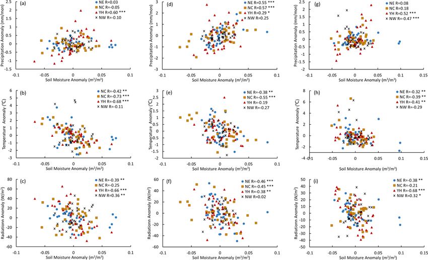
4210                     X. Ling et al.: Comprehensive evaluation of satellite-based and reanalysis soil moisture products

2013; McColl et al., 2017; Peng and Loew, 2017; Qiu et al.,        al. (2015) evaluated the ESA CCI product along with four
2018). SM can influence runoff generation, drought devel-          other data sets in Southwest China and found that it has the
opment, and many other processes of hydrology and agri-            potential to provide valuable information. Based on observa-
culture (Markewitz et al., 2010; Das et al., 2011; Sevanto et      tional data and eight model products, An et al. (2016) fur-
al., 2014; Akbar et al., 2018). Thus, understanding SM char-       ther confirmed that the CCI SM can be applied over China.
acteristics is beneficial to flood prediction (Komma et al.,       Ma et al. (2016) compared the ESA CCI and the European
2008; NorBiasto et al., 2008), drought monitoring (Dai et          Centre for Medium-Range Weather Forecasts (ECMWF)
al., 2004; Anderson et al., 2007; AghaKouchak et al., 2015;        Reanalysis– Interim (ERA-Interim) products with in situ
Li et al., 2018), and water management, which are directly         measurements and found that both products show reliable
related to crop growth (Engman, 1991; Bastiaanssen et al.,         time series results. However, few studies on long-term SM
2000; Dobriyal et al., 2012). SM also affects the climate sys-     products over 30 years have been compared with the ESA
tem through the land–atmosphere feedback loop (Kim and             CCI product using in situ measurements in East China, and
Hong, 2007; Dirmeyer, 2011; Zuo and Zhang, 2016), while            thus, more in-depth evaluation needs to be done.
the SM–climate interaction actually amplifies climate vari-           Many efforts have been made to assess the reanalysis
ability in some transitional climate zones (Seneviratne et al.,    products of soil variables based on limited observations
2010). Despite the small total mass of SM compared to other        (Decker et al., 2012; Hagan et al., 2020). Analysis of spring
water cycle components, it is essential for numerical weather      SM shows that ERA-Interim can reproduce the interan-
prediction (An et al., 2016) and has been recognized as an         nual variation in observed values well, and it exhibits a
essential climate variable (ECV; GCOS, 2010).                      better correlation with precipitation and evaporation than
   In situ measurements have been acknowledged as being            the National Centers for Environmental Prediction (NCEP)–
the most accurate method to determine SM values, but they          National Center for Atmospheric Research (NCAR) Reanal-
cannot fulfill the demand of high spatial and temporal reso-       ysis Project (R1), Modern-Era Retrospective analysis for Re-
lution for hydrometeorological use (Bárdossy and Lehmann,          search and Applications (MERRA), Japan Meteorological
1998). Furthermore, the temporal coverage of in situ mea-          Agency (JMA), or the Central Research Institute of Elec-
surements is usually not long enough. Therefore, satellite-        tric Power Industry (CRIEPI) SM products (Liu et al., 2014).
based products, reanalysis products, and numerical model           Using in situ observations from 25 networks worldwide
products are often used (Peng et al., 2017). Although model        from 1979 to 2017, ERA5 SM performs better than other
outputs are spatially and temporally continuous, large uncer-      reanalysis products, and NCEP products show higher skill in
tainties still exist in model simulations because of the phys-     terms of long-term trends (Li et al., 2020). During weak mon-
ical structure, parameters, and other reasons (Schellekens et      soon conditions, ERA-Interim overestimates SM over India,
al., 2017). Reanalysis products are generally more accurate,       and SM correlates well with observed rainfall (Shrivastava
yet they still inherit some uncertainties of the models (Berg      et al., 2017). Using 670 SM stations worldwide, Deng et
et al., 2003), and their spatial resolutions are not high enough   al. (2020) found that NCEP performed poorly in December–
for regional application (Crow and Wood, 1999). Despite the        February (DJF) and June–August (JJA) and in arid or tem-
short temporal coverage and the limitation of only measur-         perate and dry climates. Nevertheless, to our knowledge, few
ing the surface SM (Petropoulos et al., 2015), satellite-based     studies on the estimation of long time series of SM over the
products are very promising (Chauhan et al., 2003; Bogena et       Chinese mainland have been conducted.
al., 2007; de Jeu et al., 2008) because they are often based on       The objective of this study is to comprehensively evaluate
observations with high spatial resolution (Busch et al., 2012).    long-term SM products over the Chinese mainland and iden-
For this reason, satellite-based products are normally taken as    tify the most accurate products for further meteorological and
reference data sets to evaluate model outputs and reanalysis       hydrological research. For this purpose, in situ measurements
products (Crow and Ryu, 2009; Lai et al., 2014). To choose         during 1981–2013 are utilized to evaluate five SM products.
the most appropriate SM product for long-term hydrological         In addition to the comparison based on different statistical
and meteorological studies, more evaluation work needs to          metrics, the source of errors is also discussed.
be done.
   Several evaluation studies have been conducted to find a
qualified remote sensing SM product (Li et al., 2009; Zhang        2     Data and methodology
et al., 2012; Lai et al., 2014; Peng et al., 2015; An et al.,
2016; Ma et al., 2016; Zhu et al., 2018). The SM product           2.1     Remotely sensed and reanalysis products
from the European Space Agency (ESA) Climate Change
Initiative (CCI) program has attracted attention in recent         2.1.1    ESA CCI SM
years (Dorigo et al., 2018) and has been proven to have
good quality in some regions of the world (Dorigo et al.,          Generated by the ESA Program Climate Change Initiative
2015, 2017; Chakravorty et al., 2016; Ikonen et al., 2018;         CCI project (ESA CCI), the ESA CCI SM includes active,
González-Zamora et al., 2019; Beck et al., 2021). Peng et          passive, and combined products (Liu et al., 2012; Gruber et

Hydrol. Earth Syst. Sci., 25, 4209–4229, 2021                                       https://doi.org/10.5194/hess-25-4209-2021
X. Ling et al.: Comprehensive evaluation of satellite-based and reanalysis soil moisture products                           4211

al., 2017). The ESA CCI SM v04.4 combined product is em-          2.1.4    NOAA SM
ployed in this study, which provides SM data starting from
November 1978 until June 2018, with a spatial resolution of       The 20th Century Reanalysis Project (20CR) led by the
0.25◦ . The project of ESA CCI is to use C-band microwave         Earth System Research Laboratory Physical Sciences Divi-
scatterometers (Aqua satellite and the Advance Scatterome-        sion from the National Oceanic and Atmospheric Adminis-
ter, ASCAT) and multichannel microwave radiometers (i.e.,         tration (NOAA) and the University of Colorado Cooperative
SMMR, SSM/I, TMI, AMSR-E, WindSat, and AMSR2) to                  Institute for Research in Environmental Sciences (CIRES)
produce a long-term reliable time series of SM (Chakravorty       also produces a long-term SM product. The version of V2c
et al., 2016). The ESA CCI SM v04.4 is better at detect-          is used here, spanning the entire 20th century from 1851
ing SM changes (Balenzano et al., 2011) than previous ver-        to 2014 (Compo et al., 2011). The NOAA SM product is gen-
sions as it merges all active and passive level 2 products di-    erated with a spatial resolution of 2◦ at 6 h (also monthly) and
rectly to generate the combined product, rather than creat-       with four subsurface levels (0, 10, 40, and 100 cm), of which
ing active and passive products separately and then merg-         the data at 10 cm depth are used.
ing them together (ESA, 2018; Gruber et al., 2019). The
Global Land Data Assimilation System Noah (GLDAS 2.1)             2.1.5    ERA5 SM
was used as a scaling reference in the combined product to
                                                                  ERA5 is the latest reanalysis product produced by ECMWF,
obtain a consistent climatology and to flag a high vegetation
                                                                  covering the period from 1979 to the present. The product
optical depth (VOD) for SM (Dorigo et al., 2017; Pasik et
                                                                  uses a new version of the ECMWF assimilation system IFS
al., 2020). A polynomial signal-to-noise ratio (SNR) VOD
                                                                  (IFS Cycle 41R2), and combines vast amounts of historical
regression and the p value based mask was used to fill spa-
                                                                  observations, including ozone, aircraft and surface pressure
tial gaps in triple collocation analysis (TCA)-based SNR es-
                                                                  data, as well as various newly reprocessed data sets and re-
timates and exclude unreliable input data set in the combined
                                                                  cent instruments that could not be ingested in ERA-Interim
product, respectively. Here, we evaluate all the products over
                                                                  (C3S, 2017). The ERA5 model input includes the World Cli-
the period from 1981 to 2013 (the same as below), during
                                                                  mate Research Programme (WCRP) Coupled Model Inter-
which in situ measurements are also available. The top layer
                                                                  comparison Project (CMIP) for greenhouse gases, volcanic
of ESA CCI SM data at the depth of 2–5 cm depth are esti-
                                                                  eruptions, sea surface temperature (SST), and sea ice cover,
mated.
                                                                  which are appropriate for climate studies. Furthermore, the
2.1.2   ERA-Interim SM                                            spatial (31 km globally) and temporal (hourly) resolutions of
                                                                  ERA5 are rather high compared to ERA-Interim. ERA5 will
ERA-Interim is a famous reanalysis product produced by            eventually cover the period from 1950 to the present, and one
the European Centre for Medium-Range Weather Forecasts            of its key improvements is better SM (Komma et al., 2008).
(ECMWF, 2009). The data assimilation system is based on           The land surface models of the Interactions between Soil,
the Integrated Forecast System (IFS Cy31r2), which includes       Biosphere, and Atmosphere (ISBA) driven by ERA5 also
a four-dimensional analysis with a 12 h analysis window.          show consistent improvements, especially in surface SM,
The ERA-Interim data used in this study are on a fixed grid       compared to those driven by ERA-Interim (Albergel et al.,
of 80 km and have a temporal resolution of 6 h, daily, and        2018). Similar to ERA-Interim, there are levels of SM data,
monthly scales. ERA-Interim starts in 1979 and is continu-        in which the SM is interpolated to 10 cm for evaluation.
ously updated in real time (Berrisford et al., 2011). ECMWF
simulates SM at four depths, namely 0–7, 7–28, 28–100,            2.2     In situ SM and preprocessing of data sets
and 100–255 cm. As suggested by An et al. (2016), the data
                                                                  The in situ SM observations were generated by three SM data
at depths of 7–28 cm are linearly interpolated to a depth of
                                                                  sets as follows.
10 cm for evaluation.
                                                                  (1) The International Soil Moisture Network (ISMN)
2.1.3   NCEP SM
                                                                  The updated Chinese soil moisture was presented as volu-
NCEP is the second reanalysis product provided by the Na-
                                                                  metric soil moisture (θv ; cubic meters per cubic meter; here-
tional Centers for Environmental Prediction and Department
                                                                  after m3 m−3 ) for 1981 to 1999 from the ISMN website
of Energy (NCEP-DOE; Kanamitsu et al., 2002). The prod-
                                                                  (https://ismn.geo.tuwien.ac.at/en/, last access: 15 June 2020)
uct has been available since January 1979, with a spatial reso-
                                                                  (Dorigo et al., 2011). The ISMN provides a global in situ soil
lution of approximately 200 km. The temporal resolution in-
                                                                  moisture database, which have been widely used for the val-
cludes daily and monthly data. NCEP has two layers of SM
                                                                  idation of satellite products and model simulations (e.g., Al-
between 0–10 and 10–200 cm, from which the first layer was
                                                                  bergel et al., 2012). The SM data, at the depth of 0–5 and 5–
chosen for evaluation.
                                                                  10 cm, were obtained and averaged as the value at the depth
                                                                  of 0–10 cm.

https://doi.org/10.5194/hess-25-4209-2021                                       Hydrol. Earth Syst. Sci., 25, 4209–4229, 2021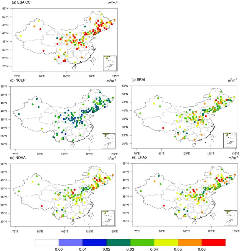
4212                       X. Ling et al.: Comprehensive evaluation of satellite-based and reanalysis soil moisture products

Figure 1. Spatial distribution of 119 agricultural–meteorological observation stations and four research regions over China for the period 1981
to 2013. The colors denote the distribution of annual precipitation (millimeters per annum; hereafter mm a−1 ) from 1971–2000.

(2) Soil water content from agricultural–meteorological                   be treated as constant. The SM mass percent was measured at
stations                                                                  11 levels, including the depths of 0–5, 5–10, 10–20, 20–30,
                                                                          30–40, 40–50, 50–60, 60–70, 70–80, 80–90, and 90–100 cm.
The in situ SM measurements are obtained from the Na-                     To match other data sets, the values at 10 cm depth are cal-
tional Meteorological Information Center of China (NMIC,                  culated by averaging the values at the depth of 5–10 and 10–
2006). The data have been collected at 778 agricultural–                  20 cm.
meteorological stations, with a temporal resolution of 10 d,                 Considering that the field capacity and the dry bulk den-
since May 1991 (on day 8, 18, and 28 of each month). As                   sity are not measured at all stations, data from 119 stations
there are too many missing observations after 2013, the eval-             are selected from 1981 to 2013. Not all in situ data were
uations of the different data sets are performed until Decem-             suitable for evaluation, given instrumental error and obser-
ber 2013. The SM data were observed at the depth of 10, 20,               vational conditions, for example, and the available measure-
50, 70, and 100 cm using drying methods, with the data at                 ment period, installation depth, and sensor placement. There-
10 cm depth being utilized. In addition, the observed SM is               fore, the evaluation was conducted in unfrozen and snow-free
expressed as the relative water content (θ 0 ; percent), while            seasons, such as June–August (JJA). The selection of appro-
the SM in all other products is in the unit of volumetric water           priate SM values is based on quality control, by removing
content (θv ; m3 m−3 ). Therefore, the observed SM is calcu-              abnormal data due to instrument failures, and threshold con-
lated by the following:                                                   trol, by retaining the value between 0–1. First, if there were
θv = θ 0 × θf × ρb /ρw ,                                         (1)      multiple data points in the same time period, then the ISMN
                                                                          SM value was selected, if available, or the average of the
where θf is the field capacity, ρb is the dry bulk density, and           remaining two data sets was calculated. Second, SM values
ρw is the water density, with a value of 1.0 (grams per cubic             greater than 3 times the standard deviation were deleted. On
centimeter; hereafter g cm−3 ).                                           considering the availability, all the in situ observations were
                                                                          averaged to monthly data at a depth of 10 cm. The distribu-
(3) Mass percent of measured SM                                           tions of the available stations are presented in Fig. 1, and
                                                                          detailed information of all the above SM products is listed in
Another data set, including SM, field capacity, and dry bulk
                                                                          Table 1.
density in China, recorded from 1981 to 1998, was obtained
from the National Meteorological Information Center of the
China Meteorological Administration. SM was presented as                  2.3   Land surface air temperature, precipitation, and
a mass percentage three times each month to avoid auxiliary                     radiation
calibration (Robock et al., 2000). The volumetric soil mois-
ture is calculated by the following:                                      The land surface air temperature and precipitation data
                                                                          are obtained from the National Meteorological Informa-
θv = θm × ρb /ρw ,                                               (2)
                                                                          tion Center (NMIC) at a spatial resolution of 0.25◦ span-
in which θm is the mass percent of measured soil moisture.                ning from 1961 to the present (http://data.cma.cn/site/index.
Within a certain period, the two parameters of θf and ρb can              html, last access: 12 March 2020). By interpolating Chi-

Hydrol. Earth Syst. Sci., 25, 4209–4229, 2021                                               https://doi.org/10.5194/hess-25-4209-2021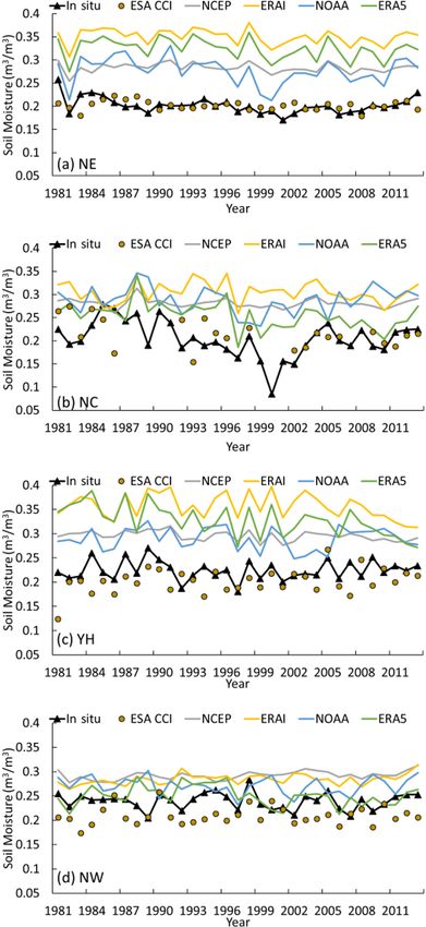
X. Ling et al.: Comprehensive evaluation of satellite-based and reanalysis soil moisture products                                     4213

Table 1. Details of the SM products used in the study.

          Name             Soil depths (cm)                  Spatial resolution          Temporal                 Temporal
                                                                                         resolution               coverage
          In situ
          ISMN             10, 20, 50, 70, 100                                           3× monthly               Jan 1981–Dec 1999
          agricultural–    10, 20, 50, 70, 100                                           3× monthly               May 1991–Dec 2013
          meteorological
          stations                                           Total 778 stations
          Mass percent     0–5, 5–10, 10–20, 20–30,          (119 used)                  3× monthly               Jan 1981–Dec 1998
          of measured      30–40, 40–50, 50–60,
          SM               60–70, 70–80, 80–90, and
                           90–100
          Satellite
          ESA CCI          −2 to 5                           0.25◦ × 0.25◦               Daily; monthly           1978–present
          Reanalysis
          ERA-Interim      0–7, 7–28, 28–100, and 100–255    0.75◦ × 0.75◦               4× daily; monthly        Jan 1979–present
          NCEP             0–10, 10–200                      T62 (−2◦ × 2◦ )             4× daily; monthly        Jan 1979–present
          NOAA             0, 10, 40, 100                    2◦ × 2◦                     8× daily; monthly        Jan 1851–Dec 2014
          ERA5             0–7, 7–28, 28–100, and 100–255    0.28125◦ × 0.28125◦         2× daily; monthly        Jan 1979–present

nese ground-based, high-density stations (over 2400 ob-
servation stations), the station observational meteorology                        n
                                                                                  P
                                                                                        xp,t − xobs,t
data set (CN05.1) includes daily mean temperature, maxi-                          t=1
mum/minimum temperature, and precipitation (Wu and Gao,               Bias =                                                           (3)
                                                                                      n
2013). The net radiation data were downloaded from the                                 Bias
ECMWF ERA5 products, for which the details can be found               rBias =                                                          (4)
                                                                              Mean(Observation)
in Sect. 2.1.5.                                                                  n
                                                                                P
   The self-calibrating Palmer drought severity index (SC-                          xobs,t − µobs xp,t − µp
PDSI) was utilized to determine the performance of all prod-                    t=1
                                                                      R= s                        s                                    (5)
ucts under different drought or wet conditions (Wells et al.,                Pn                 2 Pn           2
2004). By adjusting the climatic characteristics and calculat-                    xobs,t − µobs       xp,t − µp
                                                                               t=1                          i=1
ing the duration factors based on the characteristics of the cli-                   v
mate at a given location, the SC-PDSI has been widely used                          u n
                                                                                    uP                  2
in recent decades. The SC-PDSI fit Palmer’s 11 categories                           u     xp,t − xobs,t
                                                                                    t t=1
to allow for comparisons across time and space. A negative            RMSD =                                                           (6)
                                                                                                  n
value indicates drought conditions, and a positive value in-                            p
dicates a wet spell. The SC-PDSI data can be downloaded               ubRMSE =              RMSD2 − Bias2 ,                            (7)
via https://crudata.uea.ac.uk/cru/data/drought/#global/ (last
access: 12 January 2020).                                             in which n is the total number of time steps, xp,t and xobs,t
                                                                      are the values of SM products (including remote sensing and
2.4     Evaluation strategies                                         reanalysis) and observation at time step t, µobs and µp are
                                                                      the mean of the in situ observed values and all SM products,
2.4.1    Statistical metrics                                          and Mean(Observation) is the average of observation. The
                                                                      metrics of rBias were used to study the performance of var-
The comparisons were conducted through the statistical met-           ious regions under different drought or wet conditions. The
rics, such as the bias, relative bias (rBias), Pearson correla-       ubRMSE is introduced to evaluate temporal dynamic vari-
tion coefficient (R), root mean square difference (RMSD),             ability to remove the bias error caused by the mismatch of
and the unbiased root mean square error (ubRMSE), using               spatial representativeness between the in situ data and all
the following formulas:                                               SM products (Jackson et al., 2010, 2012; Entekhabi et al.,
                                                                      2014). What is worth saying is that the in situ observations
                                                                      were not considered as being true values because of instru-

https://doi.org/10.5194/hess-25-4209-2021                                               Hydrol. Earth Syst. Sci., 25, 4209–4229, 2021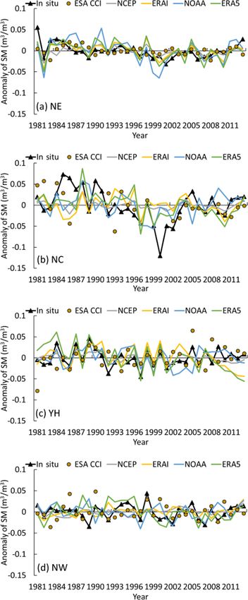
4214                      X. Ling et al.: Comprehensive evaluation of satellite-based and reanalysis soil moisture products

mental errors and representativeness, so the RMSD terminol-           Table 2. Names and spatial coverage of the selected research re-
ogy was used in this study.                                           gions.

2.4.2   Decomposition of mean square errors (MSEs)                                      Regions               Zonal    Meridional
                                                                                                           coverage     coverage
To better explain the disagreement between all the SM prod-                                                    (◦ E)        (◦ N)
ucts and in situ observations, the mean square errors (MSEs;
                                                                             I     NE   Northeast         118–130       39.5–50.5
as defined in Eq. 8) of each product in individual regions are               II    NC   North China      110–117.5        34.5–42
utilized. To decompose the MSEs, the Nash–Sutcliffe effi-                    III   YH   Yangtze–Huai      110–120       29.5–34.5
ciency (NSE; Nash and Sutcliffe, 1970) is utilized, as defined               IV    NW   Northwest         99.5–110        32.5–41
in Eq. (9).
            n
         1X                  2
MSE =          xp,t − xobs,t                                    (8)   2.5    Study area
         n t=1
             n
             P                     2                                 China is located on the eastern coast of Asia, immediately
                   xp,t − xobs,t
             t=1                               MSE                    to the west of the Pacific Ocean. It extends from roughly
NSE = 1 −    n                          = 1−    2
                                                    .           (9)   3.5 to 53.75◦ N latitude and from 73.25 to 135.25◦ E longi-
             P                     2          σobs
                   xobs,t − µobs                                      tude. Considering climate conditions and the distribution of
             t=1
                                                                      available SM data, all estimations are conducted in four re-
NSE was decomposed as the correlation, the conditional bias,          search regions, as suggested by Ma et al. (2016), which are
and the unconditional bias, as shown in Eq. (9) (Murphy,              shown in Fig. 1. Detailed information on the four research re-
1988).                                                                gions is specified in Table 2. Figure 1 also shows the annual
                                                                      mean precipitation data obtained from 160 Chinese meteoro-
NSE = A − B − C                                                       logical stations during 1971–2000 from the National Climate
                                                                      Center (NCC) of China. The 30-year averaged annual mean
A = R2
                2                                                  precipitation is treated as the climatological mean precipita-
B = R − σp /σobs                                                      tion to define the division of the climate zone.
                   2                                                  The comparisons were performed as follows: (i) find cor-
C = µp − µobs /σobs ,                                          (10)
                                                                      respondence between all SM data sets and in situ SM by us-
in which R is the correlation coefficient of observations and         ing the values at the nearest neighbor grids; (ii) compare all
products, σobs and σp are the standard deviation of in situ           the SM products at regional scales by calculating the reginal
data and all SM products. Equation (10) can be transformed            average of monthly value of all SM products, which has been
as Eq. (11), representing the correlation, bias, and variability.     proved to reduce the uncertainty caused by grid mismatch to
                                                                      some extent (Nie et al., 2008); (iii) treat all reanalysis data at
NSE = 2 · α · R − α 2 − βn2                                           the same period as missing values if the in situ observations
                                                                      are missing, and do not take these values into account.
α = σp /σobs

β = µp − µobs /σobs           .                                (11)
                                                                      3     Results and discussion
Finally, the Eq. (12) was obtained by substituting Eq. (11)
into Eq. (9) as follows:                                              3.1    Spatial pattern of SM
                                          2              2
MSE = 2σp σobs (1 − R) + σp − σobs             + µp − µobs . (12)     Figure 2 shows the spatial patterns of the 33-year aver-
                                                                      aged SM for the in situ observations and five products. ESA
The MSE was decomposed to quantify the contributions of               CCI has the highest spatial resolution, followed by ERA-
the correlation term, standard deviation term, and bias term          Interim and ERA5, and the spatial resolutions of NCEP and
(Gupta et al., 2009). On the right-hand side of the equation,         NOAA products are relatively coarse. Considering the frozen
the first term (correlation term) shows the correspondence            and vegetation cover, only the JJA SM values are used for the
between the SM product and the in situ observations. The              evaluation of the spatial pattern. Generally, most SM prod-
second term (standard deviation term) explains the degree             ucts are able to capture the overall spatial distribution of
of similarity in the variations, and the third term (bias term)       the SM value, although the NOAA SM is highly overesti-
shows the accuracy of the product. With a better understand-          mated throughout the region. According to the in situ obser-
ing of the error structure of the data sets, we can explain the       vations, SM is the lowest in the northwest and increases to
discrepancy between the SM products and the in situ obser-            the northeast and southeast. Except for NCEP, all the other
vations well (Dorigo et al., 2010).                                   data sets are able to represent the wet center in the northeast

Hydrol. Earth Syst. Sci., 25, 4209–4229, 2021                                           https://doi.org/10.5194/hess-25-4209-2021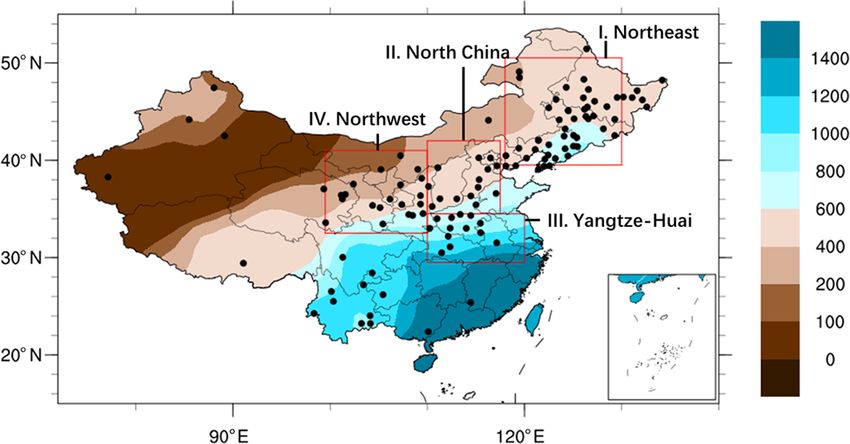
X. Ling et al.: Comprehensive evaluation of satellite-based and reanalysis soil moisture products                                      4215

Figure 2. Annual averages of (a) observations and (b–e) five satellite and reanalysis SM products (m3 m−3 ) during JJA for the period of 1981
to 2013 in China.

of China. ESA CCI underestimates SM in the north of north-               to northwest, which failed for the NCEP SM. The largest bi-
eastern China and in northwestern and southwestern China.                ases, reaching 0.15 m3 m−3 , are found in the south of north-
SM is underestimated by ESA CCI but overestimated for all                eastern China, and the largest inconsistency is found in the
the analysis data sets, except in northwestern China. For the            northwest.
ERA5 data set, the region in the north of northwestern China                The distribution of the ubRMSE for all stations is shown in
is much drier than the other products, with an average value             Fig. 3 to evaluate temporal SM dynamical variability. By re-
of less than 0.05 m3 m−3 . ERA-Interim and ERA5 SM prod-                 moving the bias, the NCEP product has the lowest ubRMSE,
ucts are able to represent the decreasing trend from southeast           with values between 0.01 and 0.03 m3 m−3 , indicating its

https://doi.org/10.5194/hess-25-4209-2021                                              Hydrol. Earth Syst. Sci., 25, 4209–4229, 2021
4216                    X. Ling et al.: Comprehensive evaluation of satellite-based and reanalysis soil moisture products

Figure 3. Same as Fig. 2 but for ubRMSE.

better performance at capturing the temporal variation in the   3.2     Temporal variability of SM
in situ SM. Large ubRMSE are found for the ESA CCI, with
values larger than 0.04 m3 m−3 , indicating that this remote    As shown in Table 2, all temporal variabilities in SM
sensing product needs to be improved at temporal variations.    are averaged over northeastern China, northern China, the
Spatially large ubRMSE are also found in the Yangtze–Huai       Yangtze–Huai region, and northwestern China, which are ab-
region and in the south of northeastern China, which may be     breviated as NE, NC, YH, and NW, respectively, below.
attributed to the high SM values. A possible explanation for
the poor performance in the northern China region might be      3.2.1    Temporal evolution
that this region is strongly influenced by irrigation.
                                                                The temporal evolutions of in situ observations and grid
                                                                point SM values from the five data sets are averaged over
                                                                each research region during JJA, as displayed in Fig. 4.

Hydrol. Earth Syst. Sci., 25, 4209–4229, 2021                                    https://doi.org/10.5194/hess-25-4209-2021
X. Ling et al.: Comprehensive evaluation of satellite-based and reanalysis soil moisture products 4217
Figure 5. Taylor diagrams of the comparison between multisource
SM products and in situ observations. The reference is the SM from
in situ observations.
research regions, while NOAA and NCEP SM have the low-
est bias among the reanalysis data sets. Reanalysis can better
reproduce the variation characteristics than remote sensing
during extreme event periods, probably due to large percent
of missing data and instrument limitations.
Table 3 shows the biases, RMSD, ubRMSE, and corre-
lation coefficients for the comparison between all products
and in situ observations during 1981 to 2013. All the eval-
uation indexes were calculated using monthly spatial aver-
age over all regions. ESA CCI presents the lowest biases for
all regions, indicating that ESA CCI is the closest to the ob-
served SM values. ERA-Interim SM has the largest positive
bias for all regions. By removing the bias error, the ubRMSE
for all products fluctuates between 0.016 and 0.025, except
for the NC region, indicating poor performance in capturing
the temporal variability. The correlation coefficient with ob-
servations for ESA CCI is relatively low. Good correlation is
obtained for ERA5 SM, except in the NC region, indicating
that ERA5 can represent the temporal and spatial variation
well. All products show a small correlation in the NC and
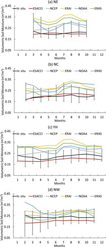
Figure 4. Time series of SM in four research regions (a–d) NW regions, implying that none of the products can capture
from 1981 to 2013. the spatiotemporal variation in SM over both regions.
The Taylor diagrams presenting the statistics of the com-
parison between ESA CCI, NCEP, ERA-Interim, NOAA,
Generally, all the reanalysis products have a positive bias ERA5, and in situ observations over four regions are shown
of 0.08–0.15, 0.05–0.10, 0.07–0.13, and 0.01–0.05 m3 m−3 in Fig. 5. Generally, the NOAA SM is highly overestimated
in the NE, NC, YH, and NW regions, respectively. ESA in all regions, and ESA CCI SM is underestimated. Most cor-
CCI tends to have a negative bias with observations be- relation coefficient values are between 0.5 and 0.6 for ERA5,
tween −0.06 and 0 m3 m−3 . All products perform well in implying a good performance with variability. Lower corre-
the NW region, and the worst performance is found in the lations are found for ESA CCI and ERA-Interim SM, demon-
NC region. ERA-Interim largely overestimates SM in all the strating that both products represent poor performance with
https://doi.org/10.5194/hess-25-4209-2021 Hydrol. Earth Syst. Sci., 25, 4209–4229, 20214218 X. Ling et al.: Comprehensive evaluation of satellite-based and reanalysis soil moisture products
Table 3. Correlation coefficients, biases, and RMSEs of the five data sets for JJA SM from 1981 to 2013. The coefficients in parentheses are
those that cannot pass the significance test (α = 0.1) with n = 33. The values marked with ∗∗ and ∗∗∗ indicate that the correlation coefficient
has passed the significance test of 95 % and 99 %, respectively. The values in brackets indicate that the significance test has not been passed.
Regions Products Bias RMSD ubRMSE Correlation
ESA CCI 0.000 0.019 0.019 (0.070)
NCEP 0.081 0.083 0.016 0.380∗∗
NE ERA-Interim 0.148 0.149 0.016 0.550∗∗∗
NOAA/CIRES 20CR 0.075 0.079 0.024 0.509∗∗∗
ERA5 0.123 0.124 0.019 0.538∗∗∗
ESA CCI −0.061 0.122 0.106 (0.122)
NCEP 0.076 0.084 0.037 (0.085)
NC ERA-Interim 0.100 0.109 0.044 (0.109)
NOAA/CIRES 20CR 0.083 0.093 0.041 (0.093)
ERA5 0.050 0.061 0.035 (0.061)
ESA CCI −0.022 0.037 0.029 (0.173)
NCEP 0.071 0.073 0.017 0.510∗∗∗
YH ERA-Interim 0.132 0.134 0.025 0.398∗∗
NOAA/CIRES 20CR 0.065 0.069 0.023 0.415∗∗
ERA5 0.103 0.107 0.027 0.535∗∗∗
ESA CCI −0.030 0.037 0.022 (0.227)
NCEP 0.053 0.056 0.019 (0.027)
NW ERA-Interim 0.045 0.049 0.020 (0.048)
NOAA/CIRES 20CR 0.032 0.039 0.023 (0.080)
ERA5 0.011 0.026 0.023 (0.244)
changing characteristics. All products exhibit poor correla- of SM in the NE region is obvious, partly due to the sufficient
tions in the NW region. water content there. Observed SM in all regions reaches its
minimum from April to June, and then increases to its max-
3.2.2 Seasonality imum from July to September, which can be reproduced by
all reanalysis. All reanalysis SM series have a larger dynamic
Monthly SM from 1981–2013 during unfrozen and snow- range than in situ observations and remote sensing SM val-
free months have also been calculated in Fig. 6, showing the ues. ERA5 is closer to the observations in the NC and NW re-
temporal evolution of SM seasonality averaged spatially over gions, while NCEP and NOAA show the smallest biases in
different regions. Overall, there exists a negative and a posi- the NE and YH regions. ERA5 SM performed better than
tive bias between remote sensing and reanalysis with respect ERA-Interim, as it shows a similar variation tendency, with
to SM observations, respectively. The difference in ESA CCI the observations, and a smaller difference, with the average
is smaller than all reanalysis products, especially in the pe- relative biases of 7.40 %, 18.70 %, 7.34 %, and 15.38 % in
riod where the in situ SM value is low, which is in line with the NE, NC, YH, and NW regions, respectively.
the findings of Ma et al. (2019), in that ESA CCI have rela- Figure 7 displays the autocorrelation coefficients lagging
tive poor skills with lower time series correlations in sparse by 1 month in different seasons to investigate the persistence
or dense VOD conditions but good performance in vegetated of the soil moisture anomalies for in situ observations and
areas that are moderately dense (Zeng et al., 2015). Further- five products. The aim of this figure is to study the soil mois-
more, soil types (silt, clay, and sand) also play an important ture memory in different seasons. It is shown from observa-
role in terms of different regions. Chakravorty et al. (2016) tions that the autocorrelation is high in spring and autumn,
studied the influence of soil texture on regional-scale perfor- indicating that the soil moisture is obviously affected by the
mance and found that large fractional RMSE is associated value from 1 month before in spring and autumn. The auto-
with a large percentage of sand, which might be one of the correlation is low in summer and winter, implying that SM in
reasons why poor performance is found in the NW region. these seasons are strongly affected by meteorological ele-
ESA CCI yields the worst seasonal cycle results with respect ments, such as the influences of liquid and solid precipitation
to temporal variation, which may be because of the large and freezing. The ESA CCI correlation are low during the
percentage of missing data. Furthermore, the remote sens- MAM (March–May), JJA, and SON (September–November)
ing products are completely independent without assimilat- seasons because of the large amount of missing data. The
ing or integrating measured observations. The seasonal cycle
Hydrol. Earth Syst. Sci., 25, 4209–4229, 2021 https://doi.org/10.5194/hess-25-4209-2021X. Ling et al.: Comprehensive evaluation of satellite-based and reanalysis soil moisture products 4219
e.g., temperature and precipitation. ERA5 shows a better per-
formance than ERA-Interim, especially with a close autocor-
relation coefficient in the NE region. The information of soil
moisture autocorrelation gives hints for the assimilation of
surface soil moisture into land surface models (Crow and
Van den Berg, 2010) in which, during summer and winter,
the influence of meteorological elements (e.g., precipitation,
temperature, evaporation, etc.) should be considered more.
3.2.3 Interannual anomalies
The JJA SM shows evident interannual anomalies in all the
research regions, as shown in Fig. 8. Most peaks and troughs
can be well represented by all products in the NE and YH re-
gions, while the variation characteristics cannot be repro-
duced in the other regions, especially in the NC region. Fur-
thermore, all products have a smaller amplitude of variation
than observations in extreme wet or drought years in the
NC and NW regions, implying that the models had a poor
ability to represent these extreme events.
Specifically, the variation range in the NOAA SM is the
largest, especially in wet and drought years in the NE region.
Taking the years of drought from 2001 to 2002 and the wet
year of 2003 as examples, this characteristic was missed by
ESA CCI. The variation range in NCEP SM is significantly
smaller than the actual measurement, and the simulation of
NCEP is obviously inferior to the other three products. In the
NC region, all products fail to capture the JJA SM variation
tendency, especially during extreme drought and wet periods.
NOAA and ERA5 can capture the basic trend, but the varia-
tion range does not match the measured value. The variation
amplitudes of NCEP and ERA-Interim are obviously smaller
than the observations. Surface SM is a variable associated
with precipitation and evaporation, both of which fluctuate
greatly with time in the JJA seasons. To improve the quality
of SM, all reanalysis data would need to improve their per-
formance in representing precipitation and evaporation, espe-
cially during extreme events. In the YH region, ERA-Interim
and ERA5 can roughly reproduce the trend of change, but
the magnitude of the change is large. There is a SM peak
Figure 6. Seasonality of SM distributions based on in situ observa-
occurring in 1998, in accordance with the 1998 floods in
tions and five products averaged over the (a) NE, (b) NC, (c) YH,
China. The peaks in the years of 1987, 1998, and 2001 can
and (d) NW regions from 1981 to 2013.
be reproduced by the all products. In the NW region, none of
these products are able to reproduce the variation character-
istics, especially with worse performances in drought periods
lowest autocorrelation coefficient is found in the NW region, than in wet periods. According to the correlation (in Table 3),
possibly because of the particular sandy soil with relative ERA5 has the best performance, but it shows a fictitious in-
high porosity and low water-holding capacity. The regions crease from 1981 to 1993.
with a good seasonal persistence of soil anomalies are lo-
cated in the NW and eastern NE regions of China, which are 3.3 Decomposition of the mean square error (MSE)
dominated by relatively simple land cover, e.g., bare soil and
forests, respectively. The NOAA SM shows larger autocor- The (a) contribution to MSE is decomposed into a correla-
relations for all seasons than the other reanalysis products, tion term, standard deviation term, and bias term according
implying that NOAA models should take into account the in- to Eq. (12), and (b) their fractions are showed in Fig. 9.
fluence of some other variables in soil moisture in the future, The contribution of the bias term is much larger than the
https://doi.org/10.5194/hess-25-4209-2021 Hydrol. Earth Syst. Sci., 25, 4209–4229, 20214220 X. Ling et al.: Comprehensive evaluation of satellite-based and reanalysis soil moisture products Figure 7. Distribution of the autocorrelation coefficient of SM in the following seasons: (a, e, i, m, q, u) FMA (February–April) and MAM (March-May), (b, f, j, n, r, v) MJJ (May–July) and JJA (June–August), (c, g, k, o, s, w) ASO (August–October) and SON (September– November), and (d, h, l, p, t, x) NDJ (November–January) and DJF (December–February) for (a–d) in situ, (e–h) ESA CCI, (i–l) NCEP, (m–p) NOAA, (q–t) ERA-Interim (ERAI), and (u–x) ERA5. Hydrol. Earth Syst. Sci., 25, 4209–4229, 2021 https://doi.org/10.5194/hess-25-4209-2021
X. Ling et al.: Comprehensive evaluation of satellite-based and reanalysis soil moisture products                                  4221

                                                                      Figure 9. The (a) decomposition of three terms to the mean
                                                                      square errors (MSEs) for the four satellite and reanalysis products
                                                                      from 1981 to 2013 and (b) their fraction.

                                                                      correlation term, except for the ESA CCI and ERA5 in the
                                                                      NW region, indicating that reducing biases is the direction
                                                                      we need to follow to further improve the quality of reanal-
                                                                      ysis SM products. The MSE of ESA CCI SM is the small-
                                                                      est for all regions, with a large fraction of the correlation
                                                                      term, indicating that the main error of ESA CCI comes from
                                                                      the poor performance of the variation tendency. The MSE
                                                                      of ERA5 performs inconsistently in that its main difference
                                                                      comes from the correlation term in the NC and NW regions,
                                                                      while the bias terms are dominant in the NE and YH regions.
                                                                      This implies that improving the spatiotemporal resolution
                                                                      and assimilating more observation might be a potential way
                                                                      to improve SM estimate, but the large fraction of ERA5 also
                                                                      points to the need to improve the model simulation ability
                                                                      of SM. Additionally, all products present poor performance
                                                                      in the NC and NW regions, with a high correlation term. The
                                                                      standard deviation term has little effect on MSE for all data
                                                                      sets, except for the ESA CCI in the NE region and ERA-
                                                                      Interim product in the NC region. The NOAA SM product
                                                                      also shows a small MSE, except in the NW regions, which is
                                                                      similar to previous evaluations in some other regions (Peng
                                                                      et al., 2015; An et al., 2016; Zhu et al., 2018).
Figure 8. Temporal evolution of the JJA SM anomaly time series
from observations and the five satellite and reanalysis products in
four research regions from 1981 to 2013.

https://doi.org/10.5194/hess-25-4209-2021                                           Hydrol. Earth Syst. Sci., 25, 4209–4229, 2021
4222 X. Ling et al.: Comprehensive evaluation of satellite-based and reanalysis soil moisture products
Figure 10. The rBias of remote sensing and reanalysis SM Figure 11. The ubRMSE of remote sensing and reanalysis SM
against in situ observations under dry or wet conditions. The against in situ observations under dry or wet conditions in differ-
dry condition consists of extreme (scPDSI < −4) and severe ent regions. The dry condition consists of extreme (scPDSI < −4)
(scPDSI < −3) drought conditions; the wet condition consists of ex- and severe (scPDSI < −3) drought conditions; the wet condition
treme (scPDSI > 4) and severe (scPDSI > 3) wet spell conditions. consists of extreme (scPDSI > 4) and severe (scPDSI > 3) wet spell
conditions.
3.4 SM performance under various climate
backgrounds ditions, indicating a better performance of all products un-
der dry conditions. The largest rBias was found for all prod-
Figure 10 shows the rBias under different humid or arid con- ucts in the NE region, implying that the largest uncertainty
ditions by utilizing SC-PDSI (Wells et al., 2004). The rBias would appear in this region during extreme events. The large
of the JJA SM between in situ observation and remote sens- difference in rBias between dry and wet conditions was ob-
ing and reanalysis was calculated at each in situ grid point served in the NW region, implying that all products fail to
as the bias divided by the mean of in situ observations and represent the SM value when the water content is high. The
then averaged over regions. All of the reanalysis products largest rBias is found for ERA-Interim under severe wet con-
show a lower rBias under drought conditions than wet con- ditions in NE, with an average bias of 144.4 %. The best per-
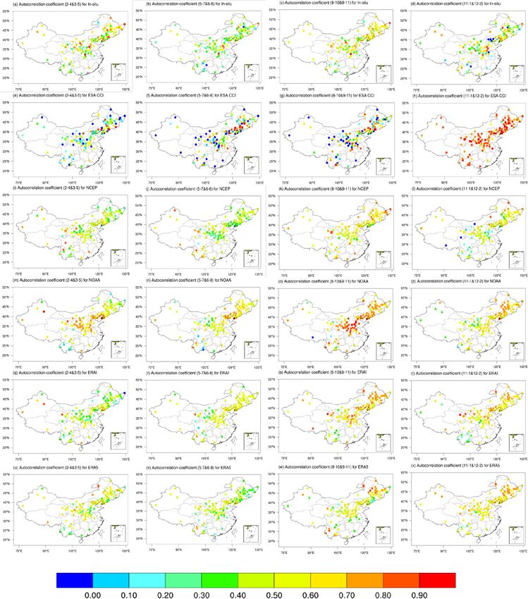
Hydrol. Earth Syst. Sci., 25, 4209–4229, 2021 https://doi.org/10.5194/hess-25-4209-2021X. Ling et al.: Comprehensive evaluation of satellite-based and reanalysis soil moisture products 4223 Figure 12. Scatterplots of monthly anomalies of (a, d, g) precipitation, (b, e, h) temperature, and (c, f, i) net radiation vs. observed soil moisture in the top 10 cm depth during 1981–2013 during (a–c) MAM, (d–f) JJA, and (g–i) SON seasons. R is the correlation coefficient over four research regions, and the values marked with ∗ , ∗∗ , and ∗∗∗ indicate that the correlation coefficient has passed the significance test of 90 %, 95 %, and 99 %, respectively. formance is found for ESA CCI SM in NW, with an average and SON seasons and in the NE and NC regions during JJA rBias of 10.0 %. season. Temperature and net radiation show a negative cor- For the ubRMSE in different regions (Fig. 11), the relation within the NE, NC, and YH regions. The correla- ubRMSE of all SM products in the NE and NW regions is tion coefficient is low for all meteorological variables in the noticeably high. The difference in ubRMSE between differ- NW region, which may be attributed to the large fraction of ent conditions is not as large as for rBias, especially in the sand there. Soil moisture in the NE and NC regions tends to NE region. Overall the ubRMSE for all products is larger un- be influenced by temperature during cold seasons. SM in the der wet conditions, while the phase is opposite in the NW re- YH region tends to be influenced by radiation during warm gion. The averaged bias for ESA CCI under drought condi- seasons, due to the large evaporation there. tions is smaller than that under wet conditions. The largest and smallest ubRMSE are found for the ESA CCI under wet 3.5 Discussion conditions in the NE region and for NCEP SM products un- der both conditions in the YH region, respectively. The ESA CCI SM product showed the top layer soil content Previous studies have shown that soil moisture is influ- up to 5 cm depth or so. The in situ measurement depth and enced by the combination of precipitation and evaporation, model output are at 0–10 cm depth, which was also treated in which land surface evaporation is linked with temperature as the top layer soil content. Such a difference would also and surface net radiation (Jasper et al., 2006; Harmsen et al., cause representativeness errors. Previous studies have found 2009). Figure 12 shows scatterplots of (a, d, g) precipitation, that there is a close relationship between surface SM and (b, e, h) temperature, and (c, f, i) net radiation anomalies ver- SM in the upper 10 cm (i.e., Albergel et al., 2008; Dorigo sus observed SM anomalies over different regions in (left et al., 2015), so the SM measurements at a depth of 10 cm column) MAM, (middle column) JJA, and (right column) were chosen as the reference to evaluate satellite-based and SON seasons. Obvious positive correlations are found be- reanalysis products. Furthermore, introducing ubRMSE and tween precipitation and SM in the YH regions during MAM conducting a comparison at the regional scale can remove https://doi.org/10.5194/hess-25-4209-2021 Hydrol. Earth Syst. Sci., 25, 4209–4229, 2021
4224                    X. Ling et al.: Comprehensive evaluation of satellite-based and reanalysis soil moisture products

the bias error caused by the mismatch of grid cells to some      east of the NW region. The large difference in soil types over
extent.                                                          the northern NW region is one of the reasons that all products
   The ESA CCI combined data generally increase the num-         show poor performance. In the NC and YH regions, sand and
ber of observations available for a time period but the cor-     clay fraction of the topsoil account for about 10 %–20 % and
relation coefficients were not better than those of the best-    30 %–50 %, 30 %–50 %, and 0 %–20 % respectively. The dif-
performing single data set (Dorigo et al., 2015). Dorigo et      ferent performance over the NC and YH regions hints that re-
al. (2015) also studied the possible reasons of input data       mote sensing and reanalysis products tend to perform worse
and found that the low correlation of the combined product,      when the soil type is sand because of its poor water retention.
possibly due to the merging procedure, including the influ-         ERA5 (∼ 0.28125◦ ) has a higher spatial resolution than
ence of vegetation (Taylor et al., 2012), the different origi-   ERA-Interim (∼ 0.75◦ ), which can be directly reflected in
nal overpass time, and the scaling of the high-resolution AS-    their spatial patterns of SM distribution. ERA5 can repro-
CAT product to lower resolution reference products. Beck         duce the spatial distribution and time series of monthly SM
et al. (2021) found that ESA CCI SM performed better in          well over the Chinese mainland in terms of low bias between
eastern Europe in terms of high-frequency fluctuations and       observations. Looking at the monthly variation and interan-
found that the reason that the overall performance of ESA        nual variation in the SM anomaly, ERA5 has a better per-
CCI may be not so good was possibly due to the incorpora-        formance than ERA-Interim in terms of low bias. It is pro-
tion of ASCAT, which performed less well. Furthermore, the       posed that ERA5 will eventually replace ERA-Interim, and
poor correlation of the remote sensing product is also associ-   we do see improvements in the ERA5 product. However,
ated with the missing of available data because of instrument    ERA5 overcorrects the problem of a small variation in ERA-
limitations and cloud impact.                                    Interim, which leads to almost the same ubRMSE and cor-
   In the winter, SM decreases in all regions, mainly because    relation coefficient in ERA5 and ERA-Interim. This implies
of decreased precipitation. Lower evaporation caused by sud-     that improving the model resolution and assimilating satel-
den cooling may explain why SM increases in early winter.        lite SM estimates can help reduce the difference in SM but
SM reaches a local minimum in the spring in most of the          will not improve much in the spatial and temporal variation at
regions, except the NE region, as a temperature rise leads       long-term scales. This might be caused by the small improve-
to higher evaporation, while precipitation does not increase     ment of assimilating the ASCAT soil moisture in the ERA5
much in this season. In the NE region, ice and melting snow      reanalysis (Hersbach et al., 2020). Beck et al. (2021) con-
partially compensate for soil water loss and help maintain       cluded that assimilating satellite soil moisture estimate may
a relatively stable SM. Increased precipitation in the sum-      not improve more than increasing model resolution or im-
mer gives rise to an evident increase in SM. In the autumn,      proving soil moisture simulation ability, which is in line with
SM continues to increase in the YH and NC regions, proba-        our results. This suggests that improving the model simula-
bly due to less evaporation caused by lower temperatures.        tion performance of SM is beneficial, especially at long-term
   Precipitation and evaporation are found to be the most        scales.
important determinants of soil moisture simulation perfor-
mance where the evaporation is associated with temperature
and radiation (Gottschalck et al., 2005; Mall et al., 2006;
Chen and Yuan, 2020). the SM value in the analysis is over-      4   Conclusions
estimated, partly due to the reason that the JJA precipitation
over China is overestimated by models (e.g., Luo et al., 2013;   To evaluate the performance of long-term SM products over
Yun et al., 2020). The largest bias in precipitation overes-     the Chinese mainland, one satellite-based product and four
timation, using the hourly 31 km resolution ERA5 reanaly-        reanalysis data sets from 1981 to 2013 are selected for com-
sis data, is found over the Tibetan and Yun-Gui plateaus, the    parison with in situ measurements at different timescales.
North China Plain, and southern China, which gives one of           Overall, ESA CCI has the best performance, with the high-
the explanations why reanalysis products represent the worst     est spatial resolution and accuracy, making it a good option
performance over the NC region.                                  for long-term hydrometeorological applications in China.
   Soil type and soil texture are also important elements for    The 0.25◦ × 0.25◦ resolution of the ESA CCI product pro-
soil moisture estimation. In the southwest of the NE region,     duces the finest spatial pattern of SM, making it more bene-
the sand fraction of the topsoil can reach about 80 %–90 %,      ficial for regional application than other SM products. How-
and the sand fraction and clay fraction of the topsoil are       ever, ESA CCI shows poor performance in terms of its low
around 30 %–40 % and 10 %–30 % respectively (Shangguan           correlation and missing values, especially in northeastern
et al., 2012) in the northern NE region. The inconsistency of    China.
the soil types over the NE region might explain why the large       ERA-Interim and ERA5 can reproduce the tendency of the
inconsistency in spatial distribution was found for all prod-    time series well and perform the best at stations, but they
ucts. In the northwest of the NW region, the sand fraction is    overestimate the seasonal variation in SM. ERA5 is also a
larger than 80 %, and the sand fraction is low in the south-     promising product, with better performance in several as-

Hydrol. Earth Syst. Sci., 25, 4209–4229, 2021                                     https://doi.org/10.5194/hess-25-4209-2021
X. Ling et al.: Comprehensive evaluation of satellite-based and reanalysis soil moisture products                                      4225

pects compared to ERA-Interim, highlighting the importance              Acknowledgements. We are grateful to all the soil moisture product
of incorporating more observations at finer spatial resolution.         developers for producing and sharing their products. We thank the
   NCEP cannot reproduce the spatial pattern of SM in                   editor, Xing Yuan, two anonymous reviewers, and Xingwang Fan,
China, the time series of NCEP SM data is poorly corre-                 for their constructive suggestions, which helped to improve this ar-
lated with observations, and the variation amplitude of its             ticle.
seasonal cycle is much larger than that of the observations.
NOAA is able to reproduce the basic spatial pattern, but it
                                                                        Disclaimer. Publisher’s note: Copernicus Publications remains
systematically overestimates SM in China and shows little
                                                                        neutral with regard to jurisdictional claims in published maps and
seasonal variation. All the SM products used in the present
                                                                        institutional affiliations.
study cannot adequately simulate the interannual variation in
the SM anomaly.
   The mismatch between SM layers in analysis products                  Financial support. This work was jointly supported by the Na-
and observations, as well as their spatial mismatch, should             tional Key R & D Program of China (grant no. 2017YFA0603803),
be investigated in the future (Choi and Hur, 2012; Crow et              the National Science Foundation of China (grant nos. 42075114,
al., 2012). Furthermore, subdaily SM model products con-                41705101, and 41775075), the Priority Academic Program
sidering the advantages of individual models under different            Development of Jiangsu Higher Education Institutions (grant
weather regimes and climate scenarios could be merged in                no. 140119001), and the ESAMOST Dragon 5 project (Monitor-
future work (Chen and Yuan, 2020).                                      ing and Modelling Climate Change in Water, Energy, and Carbon
                                                                        Cycles in the Pan-Third Pole Environment – CLIMATE-Pan-TPE).

Data availability. We acknowledge the data providers of the fol-
lowing SM products. The updated Chinese soil moisture pre-              Review statement. This paper was edited by Xing Yuan and re-
sented as volumetric soil moisture (θv ; m3 m−3 ) for 1981              viewed by two anonymous referees.
to 1999 was downloaded from the International Soil Moisture
Network website (https://ismn.geo.tuwien.ac.at/en/, last access:
15 June 2020) (ISMN, 2020). The in situ SM measurements are             References
available upon request from the website of the National Mete-
orological Information Center of China (NMIC; http://data.cma.          AghaKouchak, A., Farahmand, A., Melton, F. S., Teixeira, J., An-
cn/site/index.html, last access: 12 March 2020). We acknowledge           derson, M. C., Wardlow, B. D., and Hain, C. R.: Remote sens-
the sources of the following data sets: ESA CCI (http://www.              ing of drought: progress, challenges and opportunities, Rev.
esa-soilmoisture-cci.org, last access: 7 September 2018) (ESA,            Geophys., 53, 452–480, https://doi.org/10.1002/2014rg000456,
2018), ECMWF ERA-Interim (https://apps.ecmwf.int/datasets/                2015.
data/interim-full-daily/levtype=sfc/, last access: 5 June 2018)         Akbar, R., Gianotti, D. J. S., McColl, K. A., Haghighi, E., Salvucci,
(ECMWF, 2018), ERA5 (https://apps.ecmwf.int/data-catalogues/              G. D., and Entekhabi, D.: Estimation of landscape soil water
era5/?class=ea, last access: 27 November 2017) (ECMWF, 2017),             losses from satellite observations of soil moisture, J. Hydrom-
NCEP (https://doi.org/10.1175/BAMS-83-11-1631) (Kanamitsu et              eteorol., 19, 871–889, https://doi.org/10.1175/jhm-d-17-0200.1,
al., 2002), NOAA (https://doi.org/10.1002/qj.776) (Compo et               2018.
al., 2011), and NMIC (http://data.cma.cn/data/cdcdetail/dataCode/       Albergel, C., Rosnay, P., Gruhier, C., Munoz-Sabater, J., Hasenauer,
AGME_AB2_CHN_TEN.html, last access: 12 March 2020). The                   S., Isaksen, L., Kerr, Y., and Wagner, W.: Evaluation of remotely
land surface air temperature and precipitation data are obtained          sensed and modelled soil moisture products using global ground-
from the National Meteorological Information Center (NMIC) at             based in situ observations, Remote Sens. Environ., 118, 215–226,
a spatial resolution of 0.25◦ , spanning from 1961 to the present         https://doi.org/10.1016/j.rse.2011.11.017, 2012.
(http://data.cma.cn/site/index.html, last access: 12 October 2019).     Albergel, C., Dutra, E., Munier, S., Calvet, J. C., Munoz-
The SC-PDSI data can be downloaded via https://crudata.uea.ac.uk/         Sabater, J., de Rosnay, P., and Balsamo, G.: ERA-5 and ERA-
cru/data/drought/#global/ (last access: 12 January 2020) (Climate         interim driven ISBA land surface model simulations: which
research unit, 2020).                                                     one performs better?, Hydrol. Earth Syst. Sci., 22, 3515–3532,
                                                                          https://doi.org/10.5194/hess-22-3515-2018, 2018.
                                                                        An, R., Zhang, L., Wang, Z., Quaye-Ballard, J. A., You, J., Shen,
Author contributions. YH, WG, and JP designed the study and per-          X., Gao, W., Huang, L., Zhao, Y., and Ke, Z.: Validation of the
formed the experiments. XL and YW performed the experiments,              ESA CCI soil moisture product in China, Int. J. Appl. Earth Obs.
analyzed the data, and wrote and revised the paper. BQ, JG, KQ,           Geoinf., 48, 28–36, https://doi.org/10.1016/j.jag.2015.09.009,
and YX contributed to the interpretation of the results and the revi-     2016.
sion of the paper.                                                      Anderson, M. C., Norman, J. M., Mecikalski, J. R., Otkin, J. A.,
                                                                          and Kustas, W. P.: A climatological study of evapotranspiration
                                                                          and moisture stress across the continental United States based on
Competing interests. The authors declare that they have no conflict       thermal remote sensing: 2. Surface moisture climatology, J. Geo-
of interest.                                                              phys. Res., 112, D11112, https://doi.org/10.1029/2006jd007507,
                                                                          2007.

https://doi.org/10.5194/hess-25-4209-2021                                             Hydrol. Earth Syst. Sci., 25, 4209–4229, 2021
You can also read