PROCEEDINGS OF SPIE Confidence estimation for quantitative photoacoustic imaging - German Cancer Research Center
←
→
Page content transcription
If your browser does not render page correctly, please read the page content below
PROCEEDINGS OF SPIE
       SPIEDigitalLibrary.org/conference-proceedings-of-spie

                   Confidence estimation for
                   quantitative photoacoustic imaging

                   Janek Gröhl, Thomas Kirchner, Lena Maier-Hein

                                   Janek Gröhl, Thomas Kirchner, Lena Maier-Hein, "Confidence estimation for
                                   quantitative photoacoustic imaging," Proc. SPIE 10494, Photons Plus
                                   Ultrasound: Imaging and Sensing 2018, 104941C (19 February 2018); doi:
                                   10.1117/12.2288362

                                   Event: SPIE BiOS, 2018, San Francisco, California, United States

Downloaded From: https://www.spiedigitallibrary.org/conference-proceedings-of-spie on 8/27/2018 Terms of Use: https://www.spiedigitallibrary.org/terms-of-use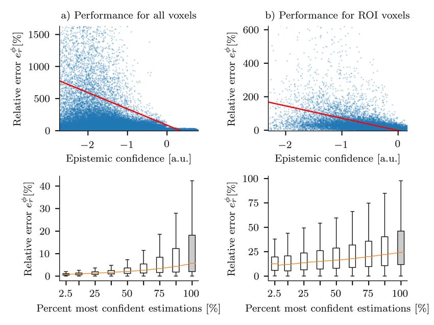
Confidence estimation for quantitative photoacoustic imaging
                                            Janek Gröhla,b , Thomas Kirchnera,c , and Lena Maier-Heina,b
                    a
                        Division of Computer Assisted Medical Interventions (CAMI), German Cancer Research
                                                  Center (DKFZ), Heidelberg, Germany
                                            b
                                              Medical Faculty, Heidelberg University, Germany
                                  c
                                    Faculty of Physics and Astronomy, Heidelberg University, Germany

                                                                                 ABSTRACT
                Quantification of photoacoustic (PA) images is one of the major challenges currently being addressed in PA
                research. Tissue properties can be quantified by correcting the recorded PA signal with an estimation of the
                corresponding fluence. Fluence estimation itself, however, is an ill-posed inverse problem which usually needs
                simplifying assumptions to be solved with state-of-the-art methods. These simplifications, as well as noise and
                artifacts in PA images reduce the accuracy of quantitative PA imaging (PAI). This reduction in accuracy is
                often localized to image regions where the assumptions do not hold true. This impedes the reconstruction of
                functional parameters when averaging over entire regions of interest (ROI). Averaging over a subset of voxels
                with a high accuracy would lead to an improved estimation of such parameters. To achieve this, we propose
                a novel approach to the local estimation of confidence in quantitative reconstructions of PA images. It makes
                use of conditional probability densities to estimate confidence intervals alongside the actual quantification. It
                encapsulates an estimation of the errors introduced by fluence estimation as well as signal noise. We validate the
                approach using Monte Carlo generated data in combination with a recently introduced machine learning-based
                approach to quantitative PAI. Our experiments show at least a two-fold improvement in quantification accuracy
                when evaluating on voxels with high confidence instead of thresholding signal intensity.
                Keywords: confidence, uncertainty estimation, quantitative imaging

                                                                          1. INTRODUCTION
                Accurate signal quantification of photoacoustic (PA) images could have a high impact on clinical PA applica-
                tions1, 2, 3 but despite of the recent progress in the field towards quantitative PA imaging (qPAI), it still remains a
                major challenge yet to be addressed.4, 5, 6, 7, 8 Optical absorption can be quantitatively extracted from a recorded
                PA signal by correcting it with an estimation of the light fluence. Fluence estimation is an ill-posed inverse
                problem that needs simplifying assumptions to be solved with state-of-the-art methods.9 A breakdown of these
                assumptions has a negative impact on the quantification result. As suggested by prior work,10, 11 a better un-
                derstanding of the underlying uncertainties of these methods could improve quantification accuracy. This is
                especially true for machine learning methods, as the space of possible optical parameter distributions is huge
                and lack of representative training data is a primary source of uncertainty.
                    In clinical applications, physicians need to be able to trust the quantification results, as high quantification
                errors could lead to unfavourable decisions for the patient. In particular, when using the quantified signal to
                derive functional parameters such as blood oxygen saturation inaccurate quantification results might lead to
                misdiagnosis. One way to attenuate this risk would be to provide an estimation of confidence that reflects the
                uncertainty alongside the quantification results. Such a confidence metric would provide the ability to decide
                whether to trust a certain result or whether to take further diagnostic steps. In an ideal case, low confidence
                values would always correspond to high quantification errors and vice versa. The estimation of uncertainty is
                vastly used in applied computer sciences12, 13, 14, 15, 16, 17, 18 and also recently in the field of PAI,10, 11, 19 but it was
                not shown how to use the acquired uncertainty information to improve the accuracy of quantification methods.
                    Further author information: (Send correspondence to J.G. or L.M.H.)
                    J.G.: E-mail: j.groehl@dkfz-heidelberg.de
                    L.M.H.: E-mail: l.maier-hein@dkfz-heidelberg.de

                               Photons Plus Ultrasound: Imaging and Sensing 2018, edited by Alexander A. Oraevsky, Lihong V. Wang, Proc.
                                  of SPIE Vol. 10494, 104941C · © 2018 SPIE · CCC code: 1605-7422/18/$18 · doi: 10.1117/12.2288362

                                                                        Proc. of SPIE Vol. 10494 104941C-1
Downloaded From: https://www.spiedigitallibrary.org/conference-proceedings-of-spie on 8/27/2018
Terms of Use: https://www.spiedigitallibrary.org/terms-of-use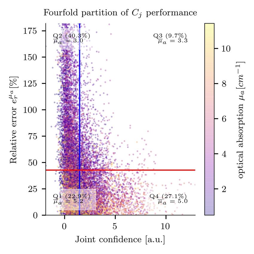
In this contribution we present a confidence metric that is able to represent quantification uncertainty in
                qPAI and thus makes it possible to improve accuracy by only evaluating confident quantification estimations. We
                quantify optical absorption in an in silico dataset with a machine learning-based approach presented previously20
                and show that using a confidence metric to threshold regions of interest can greatly improve quantification
                accuracy if the evaluation is only performed on voxels with a high confidence value.

                                                                                2. METHODS
                We use a machine learning-based model (cf. section 2.1) to derive quantitative information of optical absorption
                µa from the measured signal corresponding to the initial pressure distribution. Figure 1 illustrates that there
                are two main sources of uncertainty during the quantification process: (1) aleatoric uncertainty corresponding
                to noise and artifacts of the signal and (2) epistemic uncertainty referring to errors introduced by the quantifi-
                cation model.12, 21 As such, we propose a joint confidence metric that encompasses both epistemic as well as
                aleatoric uncertainty which can be used to choose a region of interest corresponding to contain highly confident
                quantification estimates only.
                       L

                                                             MUM
                                       se40.-
                                         AV
                             .4

                                            -      .

                Figure 1. Overview over the proposed approach to confidence estimation of quantification results. A joint confidence
                metric is proposed to select only the most confident quantification results for evaluation. The joint confidence is composed
                of an epistemic (model based) confidence metric as well as an aleatoric confidence metric that reflects the noise of the
                measured signal. In this graphic, bright and yellow colors correspond to high confidence, red tones to medium confidence,
                and darker blue colors correspond to low confidence. The signal of the initial pressure distribution is quantified using a
                quantification model presented in our previous work.20

                2.1 Signal quantification model
                Using a previously presented machine learning-based method, we estimate the fluence from a 3D signal S on
                a voxel level and use this fluence estimate to correct the signal in the imaging plane.20 In this method, we
                use feature vectors that encode both the 3D signal context of the PA image and the properties of the imaging
                system specifically for each voxel in the imaging plane. As labels we use a fluence correction term which is
                defined as φc (v) = φ(v)/φh (v), where φh (v) is a simulation based solely on a homogeneous background tissue
                assumption. During training, the model is given tuples of feature vectors and corresponding labels for each

                                                                        Proc. of SPIE Vol. 10494 104941C-2
Downloaded From: https://www.spiedigitallibrary.org/conference-proceedings-of-spie on 8/27/2018
Terms of Use: https://www.spiedigitallibrary.org/terms-of-use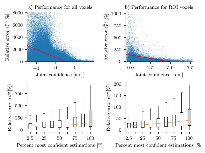
voxel in the training dataset. For quantification of a voxel v of an unseen 3D image, the voxel-specific feature
                vector is generated from the image and used to estimate the fluence φ̂(v) in that voxel with the trained model.
                The absorption coefficient µ̂a (v) is then estimated with µ̂a (v) = S(v)/(φ̂(v) · Γ) where we assume a constant
                Grueneisen coefficient Γ.
                    In this contribution, we introduce an adaptation to the previously presented quantification method in order
                to be able to represent estimation uncertainty. Our implementation of this is based on the work of Feindt13 and
                uses cumulative probability distribution functions (CDFs) as labels which allows calculating uncertainties in a
                statistically optimal way. During training, a CDF is calculated for each original fluence correction label φc (v) and
                presented to the model and when estimating previously unseen data, the model predicts a CDF corresponding to
                the feature vector and an estimate of φc (v) can be reconstructed from the 50% percentile of said CDF estimation.

                2.2 Confidence estimation
                In machine learning applications, the main sources of uncertainty can be differentiated as aleatoric uncertainty
                Ua and epistemic uncertainty Ue .12, 14, 21, 22 Ua describes the inherent noise and is introduced by the imaging
                modality, whereas Ue represents the model uncertainty mainly introduced by invalid assumptions or the lack of
                training data. In this paper we represent these uncertainties as confidence metrics C(v) on a voxel v bases, where
                lower values of C(v) represent lower confidence and higher C(v) represent higher confidence in the estimates.
                    Like any other medical imaging modality, PAT suffers from characteristic artifacts and noise pollution of
                recorded images. One way of encapsulating the noise inherent in PA images in an aleatoric confidence metric
                Ca (v) is to use the inherent contrast-to-noise ratio (CNR) for example using a definition as suggested by Welvaert
                and Rossel23

                                                                                           S(v) − µnoise
                                                                           CNR(v) =                                              (1)
                                                                                              σnoise
                with µnoise and σnoise being the mean and standard deviation of the background noise. We use this and calculate
                the standard score normalized confidence metric Ca (v) as follows:

                                                                                  CNR(v) − mean(CNR)
                                                                      Ca (v) =                                                   (2)
                                                                                       std(CNR)
                Using this definition, a low Ca (v) indicates a low contrast-to-noise ratio, which would probably lead to a high
                absorption coefficient estimation error when performing fluence correction.
                    In contrast to Ca (v), a metric of epistemic confidence Ce (v) has to reflect the model uncertainty, for example
                caused, for example, by lack of knowledge in form of labelled training data during model creation. We use two
                confidence metrics to represent the epistemic uncertainty. The first is derived from the CDFs used as labels as
                described in section 2.1. Here, the p0.8413 percentile and the p0.1587 percentile of the CDF are calculated and used
                as the left and right error intervals to encapsulate the values within one standard deviation of the mean. Thus,
                a simple measure of uncertainty derived of the error intervals is Ue1 (v) = p0.8413 (CDF(v)) − p0.1587 (CDF(v)) and
                a normalized confidence metric Ce1 (v) can be calculated with

                                                                                      Ue1 (v) − mean(Ue1 )
                                                                      Ce1 (v) = −                                                (3)
                                                                                            std(Ue1 )

                    Additionally, we use a second model to estimate the quantification performance of the proposed approach.
                In this case, to estimate a confidence metric Ce2 (v) for a previously unseen image, a random forest regressor is
                trained on feature vectors from the same training dataset DStrain as the regressor used for estimating the optical
                property of interest. However, this time the feature vectors are labeled with the relative fluence estimation error
                in the training dataset DStrain :
                                                                         |φ̂(v) − φ(v)|
                                                            Etrain (v) =                                                        (4)
                                                                              φ(v)

                                                                        Proc. of SPIE Vol. 10494 104941C-3
Downloaded From: https://www.spiedigitallibrary.org/conference-proceedings-of-spie on 8/27/2018
Terms of Use: https://www.spiedigitallibrary.org/terms-of-use
where φ(v) is the ground truth fluence in v and φ̂(v) is the fluence estimated by the model. Normalized estimations
Êtrain (v) of this error can then be used as confidence metric Ce2 (v) with
Êtrain (v) − mean(Etrain )
Ce2 (v) = − (5)
std(Etrain )
where Etrain = {eφr (v 0 )|v 0 ∈ Vtrain } is the set of all relative fluence estimation errors in DStrain with voxels Vtrain .
The parameters of the regressor for confidence estimation are set to the same values as those of the first regressor.
In order to give one global confidence estimate for a single voxel estimation, the presented metrics need to
be combined into one. As both Ce1 and Ce2 are estimates for the epistemic confidence of the machine learning
algorithm, the average of both confidence estimates is calculated and interpreted as a metric of the overall
epistemic confidence:
Ce1 (v) + Ce2 (v)
Ce (v) = (6)
2
To combine the epistemic and aleatoric confidence metric into one joint confidence metric Cj , the epistemic
and aleatoric confidence measures are averaged as well. This is possible, as both Ca (v) and Ce (v) are in the
same value range after the application of standard score normalization.
Ca (v) + Ce (v)
Cj (v) = (7)
2
2.3 Experiment
The purpose of our experiment is to validate whether incorporating the proposed confidence metric provides a
benefit in terms of fluence estimation and absorption quantification accuracy. We use an in silico dataset for
training of the machine learning algorithm. The dataset consists of multiple vessels in a homogeneous background.
In each volume there are 1−7 vessels that have a radius of 0.5−6 mm and an absorption coefficient range of 1−12
cm−1 . Light propagation is simulated using an adaptation of the widely used Monte Carlo framework mcxyz by
Steve Jacques.24 After simulation of the initial pressure distribution, we apply a Gaussian noise model with an
additive component with a mean and std of 5 ± 5 a.u. corresponding to the average signal and a multiplicative
component of 3%. This is done to resemble the noise levels commonly seen with our PA scanner.
For the concrete implementation of the epistemic confidence we followed the suggestions by Feindt13 and use
100 sample points of the corresponding CDF as a label for the model. As the model we use the python scikit-
learn25 random forest implementation to estimate a CDF according to a given feature vector. During estimation,
the fluence value can be reconstructed from the 50% percentile of the estimated CDF. Due to the nature of our
data, we performed data augmentation by converting the label range into a logarithmic scale and sampled equally
from the resulting distribution. At sampling time, we also applied random 20% white multiplicative Gaussian
noise permutations of the feature vector for each sampled data item to prevent overfitting.
For hyperparameter adjustment, we monitor the training process on a validation dataset and report results
on a separate test dataset. We evaluate the performance of the defined confidence metrics on all voxels as well
as voxels in a certain region of interest (ROI), which is defined as all voxels within vessel structures with a CNR
>= 2 as in previous work20 where also more detailed information on the dataset simulation can be found.
Proc. of SPIE Vol. 10494 104941C-4
Downloaded From: https://www.spiedigitallibrary.org/conference-proceedings-of-spie on 8/27/2018
Terms of Use: https://www.spiedigitallibrary.org/terms-of-use3. RESULTS
We report quantitative results for both fluence estimation as well as absorption quantification and we define the
relative fluence estimation error as eφr and the relative absorption quantification error as eµr a . As the epistemic
confidence metric Ce should be positively correlated with the relative fluence estimation error eφr , because it is
a measure of the uncertainty introduced by the machine learning model, we first evaluate the top n % confident
samples according to Ce in section 3.1 and afterwards we evaluate the top n % confident absorption quantifica-
tions according to the joint confidence metric Cj in section 3.2. Figure 2 shows representative example images
displaying examples of the epistemic as well as the joint confidence metric from the test dataset with the overall
highest, lowest and median relative fluence estimation error in the CNR based region of interest (ROI).
(1) Relative error e (2) Epistemic confidence Ce (3) Relative error era (4) Joint confidence C3
0- 0 0 0-
E 10 - 10 10 10 -
20 - 20 20 20 -
Q
0 50 100 150 200 -3 -2 -1 0 1 0 50 100 150 200 -1 0 1 2 3 4
Relative error 4(%) Epistemic confidence [a.u.] Relative error era( %) Joint confidence [a.u.]
(a) Image with the lowest relative error
(1) Relative error e (2) Epistemic confidence Ce (3) Relative error er° (4) Joint confidence C.,
0 0 0 -.s r 0-
ff
E 10- 10 10- 10-
4
20 - 20 : 20 -r;_v' 20 -
0 50 100 150 200 -3 -2 -1 0 1 0 50 100 150 200 -1 0 1 2 3 4
Relative error 4(%) Epistemic confidence [a.u.] Relative error era( %) Joint confidence [a.u.]
(b) Image with median relative error
(1) Relative error e (2) Epistemic confidence Ce (3) Relative error (4) Joint confidence C3
0 0- 0- 0-
E 10 10 - 10 - 10 -
5
20 20 - -11111111010111 20 - 20 -
0 50 100 150 200 -3 -2 -1 0 1 0 50 100 150 200 -1 0 1 2 3 4
Relative error 4(%) Epistemic confidence [a.u.] Relative error era( %) Joint confidence [a.u.]
(c) Image with the highest relative error
Figure 2. Representative example images from the test dataset with the overall highest, lowest and median relative
fluence estimation error in the CNR based region of interest (ROI). From left to right: (1) the relative fluence estimation
error as well as (2) the corresponding epistemic confidence metric, (3) the relative absorption quantification error, and (4)
the corresponding joint confidence metric. In (1) and (3) the darker shades of red correspond to higher relative estimation
errors and in (2) and (4) high confidence corresponds to brighter yellow and orange colors whereas lower confidence values
correspond to darker red and purple colors.
Proc. of SPIE Vol. 10494 104941C-5
Downloaded From: https://www.spiedigitallibrary.org/conference-proceedings-of-spie on 8/27/2018
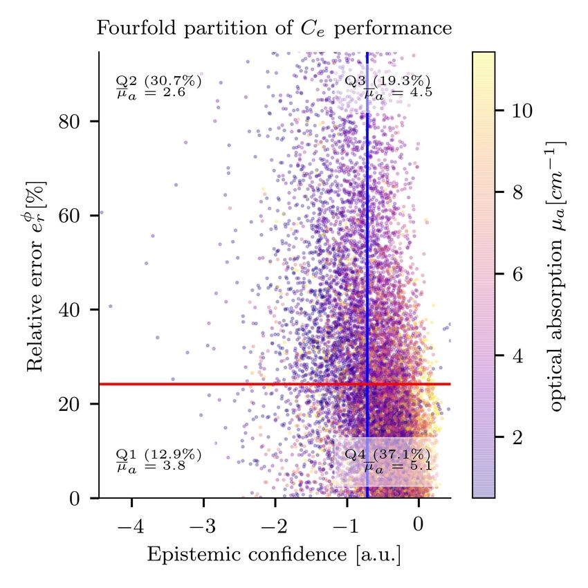
Terms of Use: https://www.spiedigitallibrary.org/terms-of-use3.1 Epistemic confidence metric for fluence estimation
When considering all voxels, the results in this work correspond with the results presented in our previous work20
for the high noise, multivessel dataset. In evaluation of the 2.5% most confident estimations, the median relative
fluence estimation error eφr over ROI dropped by up to 12 percentage points to 12% and by up to 5 percentage
points to 0.7% when evaluating over all voxels (see figure 3).
b) Performance for ROI voxels
600
-e
ó 400
-2 -1 0 -2 -1 0
Epistemic confidence [a.u.] Epistemic confidence [a.u.]
100 -
75 -
50 -
25 -
0- 0-
2.5 25 50 75 100 2.5 25 50 75 100
Percent most confident estimations [ %] Percent most confident estimations [%]
Figure 3. Evaluation of top n percent most confident estimations only. The top scatterplot shows the distribution of the
relative estimation error in relation to the confidence measure. The boxplots demonstrate the distributions of the 2.5% to
100% most confident voxels. a) is evaluated over all voxels whereas b) shows the results when evaluating only over ROI
voxels. In both cases there is an increasing improvement when evaluating over fewer more confident estimates. The red
line represents the trendline of the data and the orange line plots the median errors.
3.2 Joint confidence metric for absorption reconstruction
The accuracy of absorption quantification is dependent on both the fluence estimation error as well as the noise
of the PA image. Due to this dependency, the quantification error should be dependent on both the epistemic
and the aleatoric confidence metrics.
We perform this evaluation by relating the relative absorption quantification error eµr a to the joint confidence
metric Cj . When evaluating over the 2.5% most confident estimations, eµr a over ROI voxels dropped by 24
percentage points to 17% and by 107 percentage points to 41% when evaluating over all voxels (see figure 4).
3.3 Fourfold partitioning analysis of confidence metrics
In order to gain a better understanding of the properties of the presented confidence metrics we did a fourfold
partitioning of their respective performances in the ROI (cf. fig. 5). When using the mean confidence and
the median relative error as the partitioning values, the analysis revealed that for both metrics, nearly 70%
of the tuples are either located in the high confidence low error or the low confidence high error quadrant.
The remaining 30% of tuples are distributed in the other quadrants. The calculation of the mean absorption
coefficients of each quadrant reveals that there is a positive correlation between the epistemic confidence and the
absorption coefficient in fluence estimation as well as a negative correlation between the absorption coefficient
and the absorption estimation error.
Proc. of SPIE Vol. 10494 104941C-6
Downloaded From: https://www.spiedigitallibrary.org/conference-proceedings-of-spie on 8/27/2018
Terms of Use: https://www.spiedigitallibrary.org/terms-of-usea) Performance for all voxels b) Performance for ROI voxels
8000 1000
a
6000 Q)
750
0
4000 500
2000 tal
250
f:4
-1 0 1 0.0 2.5 5.0 7.5
Joint confidence [a.u.] Joint confidence [a.u.]
200
F
150
100
a)
? 250 - 50
0
2.5
1 I 25 50 75 100
Percent most confident estimations [R] Percent most confident estimations [R]
Figure 4. Evaluation of the n percent most confident quantifications over a) all and b) ROI voxels according to the joint
confidence metric Cj . The distributions of the 2.5% to 100% most confident voxels are shown in boxplots. The red line
represents the trendline of the data and the orange line plots the median errors.
Fourfold partition of Ci performance
175 -} Q3 (9.7 %1
ua =3.
-10 - 10
150
-6
4
50
A
-2 25 2
-4 -3 -2 -1 0 0 5 10
Epistemic confidence [a.u.] Joint confidence [a.u.]
Figure 5. Fourfold partition of the (1) epistemic confidence metric and the relative fluence estimation error eφr as well as
the (2) joint confidence metric and the absorption estimation error eµa
r in the ROI. The blue line represents is positioned at
the mean confidence value and the red line is positioned at the median relative error. Nearly 70% of all tuples are located
in Q2 and Q4, while 30% are located in Q1 and Q3. The color coding of the tuples corresponds to the corresponding
optical absorption property.
Proc. of SPIE Vol. 10494 104941C-7
Downloaded From: https://www.spiedigitallibrary.org/conference-proceedings-of-spie on 8/27/2018
Terms of Use: https://www.spiedigitallibrary.org/terms-of-use4. DISCUSSION
The presented approach to confidence estimation provides a means to combine both epistemic and aleatoric
confidences in a joint confidence metric for quantitative photoacoustic imaging. It would be a valuable tool for
providing quantification results only for voxels with low estimated error. In this context, the tradeoff between
the percentage of confident voxels and the increase in accuracy must be considered. It is worth noting that
even a small percentage of very accurately quantified voxels can be utilized to obtain an improved measure of
optical absorption or oxygenation in a region, as estimating optical and functional properties in larger regions
is common in many imaging systems (cf. e.g.26, 27 ). Doing so can yield an improvement over the practice of
thresholding based on simply the signal intensity. In this contribution we suggest using the CNR as a metric
for the aleatoric confidence. However, it is entirely possible to also use other signal-to-noise or contrast-to-noise
metrics as defined by Welvaert and Rossel.23 Completely different approaches as described by e.g. Kendall and
Gal12 are also viable. Figure 4 shows that the joint confidence metric might not be ideal when evaluating over
all voxels and not over the pre-selected ROI. It is the intention of this project to provide thorough investigation
into this aspect in future research. This is imperative, especially considering the rise in median error just before
when evaluating on more than 2.5% but less than 10% of all voxels. This is most likely due to the fact that we
calculate the CNR using the mean and std noise of the entire image. As such, this could be improved by using a
separate noise model for each individual pixel in the imaging plane. Visualization of the joint confidence metric
in figure 2 shows that the aleatoric confidence metric seems to outweigh the model-based confidence metric.
This is understandable, as the proposed quantification strategy in fact amplifies additive noise components in
regions with a low CNR. In this context it needs to be kept in mind that there are countless possible strategies
of combining both the epistemic and aleatoric confidence metric and there may be aggregations favourable to
the one presented in this work. The fourfold partitioning analysis shows the strengths and weaknesses of the
proposed approach. The quadrants Q2 and Q4 are the quadrants representing high confidence and low error or
low confidence and high error. While most confidence-error tuples are located in these quadrants, about 30%
of all tuples are not. These are distributed into the two remaining quadrants: Q1 containing low confidence
and low error and Q3 containing high confidence and high error. Cases where high errors are assigned a high
confidence value can be very critical and thus need to be minimized. Using the joint confidence metric, these
cases could be reduced from 19% to 10% with respect to using the epistemic confidence metric only. The
proposed confidence metrics can potentially be provided in real-time, as they are directly derivable from either
the PA image or the CDF estimates. An open question for future research is how to find a means of enabling
a quantitative and data-independent interpretation of the proposed joint confidence metric. As in the currently
proposed implementation the individual metrics are normalized over the entire test set before aggregation into
the joint confidence Cj metric, the only practical approach is to consider a certain percentage of confident voxels,
regardless of their actual value. However, it would be much more convenient to be able to have a fixed value
range, wherein a certain value always corresponds to a high or low confidence estimation. This would enable
calculation of matchable certainty estimates for any new quantification result. Furthermore, it has to be analyzed
how the proposed epistemic confidence metric performs for hand-picked factitious tissue properties that were not
included in the original training set. A thorough analysis of different quantification models in combination with
the proposed confidence metrics would also be of interest.
The results of the performed experiment show that evaluation of a subset of very confident estimates can
drastically improve accuracy. The validation was performed on Monte Carlo simulated in silico data, but if our
findings hold true in vitro and in vivo, real-time provision of confidence metrics could prove to be an invaluable
tool for clinical applications of qPAI.
ACKNOWLEDGMENTS
The authors would like to acknowledge support from the European Union through the ERC starting grant
COMBIOSCOPY under the New Horizon Framework Programme grant agreement ERC-2015-StG-37960. The
authors would also like to thank the ITCF of the DKFZ for the provision of their computing cluster.
Proc. of SPIE Vol. 10494 104941C-8
Downloaded From: https://www.spiedigitallibrary.org/conference-proceedings-of-spie on 8/27/2018
Terms of Use: https://www.spiedigitallibrary.org/terms-of-useREFERENCES
[1] Cox, B., Laufer, J. G., Arridge, S. R., and Beard, P. C., “Quantitative spectroscopic photoacoustic imaging:
a review,” Journal of biomedical optics 17(6), 0612021–06120222 (2012).
[2] Xu, M. and Wang, L. V., “Photoacoustic imaging in biomedicine,” Review of scientific instruments 77(4),
041101 (2006).
[3] Ntziachristos, V., “Going deeper than microscopy: the optical imaging frontier in biology,” Nature Meth-
ods 7, 603–614 (Aug. 2010).
[4] Elbau, P., Mindrinos, L., and Scherzer, O., “Quantitative reconstructions in multi-modal photoacoustic and
optical coherence tomography imaging,” Inverse Problems (2017).
[5] Kaplan, B., Buchmann, J., Prohaska, S., and Laufer, J., “Monte-Carlo-based inversion scheme for 3d quan-
titative photoacoustic tomography,” Proceedings of the SPIE, Volume 10064, id. 100645J 13 pp.(2017). 64
(2017).
[6] Tarvainen, T., Pulkkinen, A., Cox, B. T., and Arridge, S. R., “Utilising the radiative transfer equation in
quantitative photoacoustic tomography,” 10064, 100643E–100643E–8 (2017).
[7] Brochu, F. M., Brunker, J., Joseph, J., Tomaszewski, M. R., Morscher, S., and Bohndiek, S. E., “Towards
Quantitative Evaluation of Tissue Absorption Coefficients Using Light Fluence Correction in Optoacoustic
Tomography,” IEEE Transactions on Medical Imaging 36, 322–331 (Jan. 2017).
[8] Haltmeier, M., Neumann, L., Nguyen, L. V., and Rabanser, S., “Analysis of the Linearized Problem of
Quantitative Photoacoustic Tomography,” arXiv preprint arXiv:1702.04560 (2017).
[9] An, L., Saratoon, T., Fonseca, M., Ellwood, R., and Cox, B., “Statistical independence in nonlinear model-
based inversion for quantitative photoacoustic tomography,” Biomedical Optics Express 8, 5297–5310 (Nov.
2017).
[10] Fonseca, M., Saratoon, T., Zeqiri, B., Beard, P., and Cox, B., “Sensitivity of quantitative photoacoustic
tomography inversion schemes to experimental uncertainty,” in [SPIE BiOS ], 97084X–97084X, International
Society for Optics and Photonics (2016).
[11] Pulkkinen, A., Cox, B. T., Arridge, S. R., Kaipio, J. P., and Tarvainen, T., “Estimation and uncertainty
quantification of optical properties directly from the photoacoustic time series,” 10064, 100643N–100643N–7
(2017).
[12] Kendall, A. and Gal, Y., “What Uncertainties Do We Need in Bayesian Deep Learning for Computer
Vision?,” arXiv:1703.04977 [cs] (Mar. 2017).
[13] Feindt, M., “A Neural Bayesian Estimator for Conditional Probability Densities,” arXiv:physics/0402093
(Feb. 2004).
[14] Senge, R., Bösner, S., Dembczyski, K., Haasenritter, J., Hirsch, O., Donner-Banzhoff, N., and Hüllermeier,
E., “Reliable classification: Learning classifiers that distinguish aleatoric and epistemic uncertainty,” Infor-
mation Sciences 255, 16–29 (Jan. 2014).
[15] Gal, Y., Islam, R., and Ghahramani, Z., “Deep Bayesian Active Learning with Image Data,”
arXiv:1703.02910 [cs, stat] (Mar. 2017).
[16] Choi, S., Lee, K., Lim, S., and Oh, S., “Uncertainty-Aware Learning from Demonstration using Mixture
Density Networks with Sampling-Free Variance Modeling,” arXiv:1709.02249 [cs] (Sept. 2017).
[17] Maier-Hein, L., Ross, T., Gröhl, J., Glocker, B., Bodenstedt, S., Stock, C., Heim, E., Götz, M., Wirkert,
S., Kenngott, H., and others, “Crowd-algorithm collaboration for large-scale endoscopic image annotation
with confidence,” in [International Conference on Medical Image Computing and Computer-Assisted Inter-
vention ], 616–623, Springer (2016).
[18] Moccia, S., Wirkert, S. J., Kenngott, H., Vemuri, A. S., Apitz, M., Mayer, B., De Momi, E., Mattos,
L. S., and Maier-Hein, L., “Uncertainty-Aware Organ Classification for Surgical Data Science Applications
in Laparoscopy,” arXiv:1706.07002 [cs] (June 2017). arXiv: 1706.07002.
[19] Tarvainen, T., Pulkkinen, A., Cox, B. T., Kaipio, J. P., and Arridge, S. R., “Image reconstruction with
noise and error modelling in quantitative photoacoustic tomography,” in [SPIE BiOS], 97083Q–97083Q,
International Society for Optics and Photonics (2016).
[20] Kirchner, T., Gröhl, J., and Maier-Hein, L., “Local context encoding enables machine learning-based quan-
titative photoacoustics,” arXiv:1706.03595 [physics] (June 2017).
Proc. of SPIE Vol. 10494 104941C-9
Downloaded From: https://www.spiedigitallibrary.org/conference-proceedings-of-spie on 8/27/2018
Terms of Use: https://www.spiedigitallibrary.org/terms-of-use[21] Urbina, A., Mahadevan, S., and Paez, T. L., “Quantification of margins and uncertainties of complex
systems in the presence of aleatoric and epistemic uncertainty,” Reliability Engineering & System Safety 96,
1114–1125 (Sept. 2011).
[22] Chowdhary, K. and Dupuis, P., “Distinguishing and integrating aleatoric and epistemic variation in uncer-
tainty quantification,” ESAIM: Mathematical Modelling and Numerical Analysis 47, 635–662 (May 2013).
[23] Welvaert, M. and Rosseel, Y., “On the Definition of Signal-To-Noise Ratio and Contrast-To-Noise Ratio for
fMRI Data,” PLOS ONE 8, e77089 (June 2013).
[24] Jacques, S. L., “Coupling 3d Monte Carlo light transport in optically heterogeneous tissues to photoacoustic
signal generation,” Photoacoustics 2(4), 137–142 (2014).
[25] Pedregosa, F., Varoquaux, G., Gramfort, A., Michel, V., Thirion, B., Grisel, O., Blondel, M., Prettenhofer,
P., Weiss, R., Dubourg, V., and others, “Scikit-learn: Machine learning in Python,” Journal of Machine
Learning Research 12(Oct), 2825–2830 (2011).
[26] Tzoumas, S., Nunes, A., Olefir, I., Stangl, S., Symvoulidis, P., Glasl, S., Bayer, C., Multhoff, G., and
Ntziachristos, V., “Eigenspectra optoacoustic tomography achieves quantitative blood oxygenation imaging
deep in tissues,” Nature Communications 7, 12121 (June 2016).
[27] Valluru, K. S., Wilson, K. E., and Willmann, J. K., “Photoacoustic Imaging in Oncology: Translational
Preclinical and Early Clinical Experience,” Radiology 280, 332–349 (July 2016).
Proc. of SPIE Vol. 10494 104941C-10
Downloaded From: https://www.spiedigitallibrary.org/conference-proceedings-of-spie on 8/27/2018
Terms of Use: https://www.spiedigitallibrary.org/terms-of-useYou can also read