Contributions of advection and melting processes to the decline in sea ice in the Pacific sector of the Arctic Ocean - The Cryosphere
←
→
Page content transcription
If your browser does not render page correctly, please read the page content below
The Cryosphere, 13, 1423–1439, 2019
https://doi.org/10.5194/tc-13-1423-2019
© Author(s) 2019. This work is distributed under
the Creative Commons Attribution 4.0 License.

Contributions of advection and melting processes to the decline in
sea ice in the Pacific sector of the Arctic Ocean
Haibo Bi1,2,3,4 , Qinghua Yang5,6,7 , Xi Liang8 , Liang Zhang1,2,3,4 , Yunhe Wang1,2,3,4 , Yu Liang1,2,3,4 , and
Haijun Huang1,2,3,4
1 Key  laboratory of Marine Geology and Environment, Institute of Oceanology,
Chinese Academy of Sciences, Qingdao, China
2 Laboratory for Marine Geology, Qingdao National Laboratory for Marine Science and Technology, Qingdao, China
3 Center for Ocean Mega-Science, Chinese Academy of Sciences, Qingdao, China
4 College of Earth and Planetary Science, University of Chinese Academy of Sciences, Beijing, China
5 Guangdong Province Key Laboratory for Climate Change and Natural Disaster Studies,

School of Atmospheric Sciences, Sun Yat-sen University, Zhuhai, China
6 State Key Laboratory of Numerical Modeling for Atmospheric Sciences and Geophysical Fluid Dynamics,

Institute of Atmospheric Physics (IAP), Chinese Academy of Sciences, Beijing, China
7 Southern Marine Science and Engineering Guangdong Laboratory (Zhuhai), Zhuhai, China
8 Key Laboratory of Research on Marine Hazards Forecasting, National Marine Environmental Forecasting Center,

Beijing, China

Correspondence: Haibo Bi (bhb@qdio.ac.cn)

Received: 15 January 2019 – Discussion started: 22 January 2019
Revised: 9 April 2019 – Accepted: 17 April 2019 – Published: 8 May 2019

Abstract. The Pacific sector of the Arctic Ocean (PA, here-        counts for 90.4 % of the sea ice retreat in the PA in sum-
after) is a region sensitive to climate change. Given the          mer, whereas the remaining 9.6 % is explained by the outflow
alarming changes in sea ice cover during recent years, knowl-      process, on average. Moreover, our analysis suggests that
edge of sea ice loss with respect to ice advection and melting     the connections are relatively strong (R = 0.63), moderate
processes has become critical. With satellite-derived prod-        (R = −0.46), and weak (R = −0.24) between retreat of sea
ucts from the National Snow and Ice Center (NSIDC), a              ice and the winds associated with the dipole anomaly (DA),
38-year record (1979–2016) of the loss in sea ice area in          North Atlantic Oscillation (NAO), and Arctic Oscillation
summer within the Pacific-Arctic (PA) sector due to the two        (AO), respectively. The DA participates by impacting both
processes is obtained. The average sea ice outflow from the        the advection (R = 0.74) and melting (R = 0.55) processes,
PA to the Atlantic-Arctic (AA) Ocean during the summer             whereas the NAO affects the melting process (R = −0.46).
season (June–September) reaches 0.173 × 10⁶ km2 , which
corresponds to approximately 34 % of the mean annual ex-
port (October to September). Over the investigated period,
a positive trend of 0.004 × 10⁶ km2 yr−1 is also observed          1   Introduction
for the outflow field in summer. The mean estimate of sea
ice retreat within the PA associated with summer melting is        As the Arctic climate warms (Comiso, 2010; Overland et
1.66×10⁶ km2 , with a positive trend of 0.053×10⁶ km2 yr−1 .       al., 2010; Graham et al., 2017), a wide range of researchers
As a result, the increasing trends of ice retreat caused by out-   and the public show compelling interest in topics associated
flow and melting together contribute to a stronger decrease        with the drop in sea ice coverage (Kay and Gettelman, 2009;
in sea ice coverage within the PA (0.057 × 10⁶ km2 yr−1 )          Spreen et al., 2009, 2011; Polyakov et al., 2010; Zhang et
in summer. In percentage terms, the melting process ac-            al., 2010; Woods et al., 2013; Tjernström et al., 2015; Notz
                                                                   and Stroeve, 2016; Screen and Francis, 2016; Koyama et al.,

Published by Copernicus Publications on behalf of the European Geosciences Union.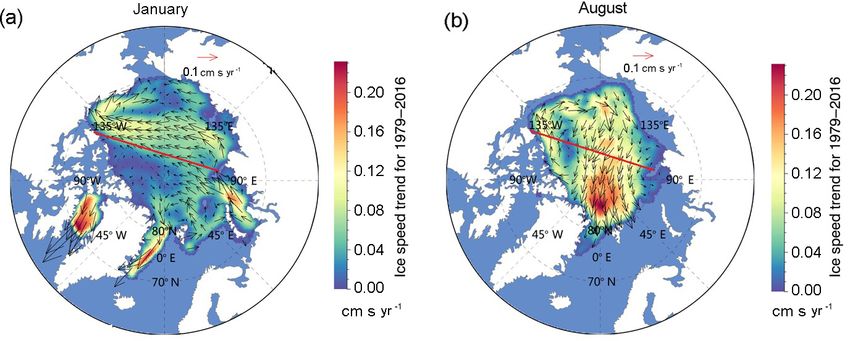
1424                                 H. Bi et al.: Contributions of advection and melting processes to the decline in sea ice

2017; Smedsrud et al., 2017; Stroeve et al., 2017; Nieder-         2013). Consequently, advective sea ice mass balance within
drenk and Notz, 2018). For the period since the late 1970s,        the Arctic Ocean may have been changing.
sea ice extent has been decreasing as revealed from a series          Although we are familiar with the fact that the sea ice
of satellite microwave observations, ranging from −0.45 to         mass balance is closely related to the dynamic (advection)
−0.39 % yr−1 depending on different data products (Comiso          and thermodynamic (melting) processes, quantitative knowl-
et al., 2017). Specifically, the September Arctic sea ice extent   edge about their contributions to the sea ice area changes
has been found to be the month with the most rapid decrease        within the Arctic Ocean is scarce. In addition the utilization
, at approximately −1.30 % yr−1 for the period 1979–2017.          of satellite observations, modeling studies have been com-
   Comiso (2011) reported a more negative trend in the             monly used to diagnose the dynamic and thermodynamic
multiyear ice (MYI) coverage, approximately −1.72 % yr−1           forcing (e.g., Lindsay et al., 2009). In this study, we exam-
in winter over the period 1979–2011. As a result, the              ine the contributions of these two processes to the sea ice
MYI extent decreased from approximately 6.2 × 10⁶ km2              depletion within the PA side where sea ice loss is the most
in the 1980s to only 2.8 × 10⁶ km2 in the late 2000s.              pronounced during summer (Cavalieri and Parkinson, 2012;
Recently, record lows in sea ice extent have been fre-             Kawaguchi et al., 2014; Lynch et al., 2016; Comiso et al.,
quently set in summer over the past years (Serreze et al.,         2017). In a preceding investigation, Kwok (2008a) examined
2003; Parkinson and Comiso, 2013; Stroeve et al., 2013).           the sea ice retreat within the PA sector due to melting and ad-
According to the National Snow and Ice Data Center                 vection in the summers of 2003–2007. However, the record
(NSIDC) report (http://nsidc.org/arcticseaicenews/2012/09/         of 5 years is too short to draw any robust conclusion about
arctic-sea-ice-extent-settles-at-record-seasonal-minimum/,         the variability and trend in the sea ice area changes due to the
last access: 7 May 2019), the Arctic sea ice extent plum-          two processes. Kwok (2008b) investigated the sea ice trans-
meted to its minimum of 3.41 × 10⁶ km2 on 16 September             port between the PA and Atlantic-Arctic (AA) sectors for the
2012, approximately 18 % below the previous record min-            period 1979–2007. However, the contribution of ice melting
imum in 2007. The significant decline in sea ice coverage          to sea ice decline in PA is beyond the scope of their study.
in summer implies that less Arctic sea ice can survive the         Taking advantage of a longer and updated version of sea ice
melting season to replenish the MYI cover in September             motion data provided by the NSIDC, this study attempts to
(Kwok, 2007). Therefore, the Arctic Ocean is now domi-             quantify the contributions of the two processes (advection
nated by younger and thinner first-year ice (FYI) (Maslanik        and melting) to the retreat of sea ice in summer within the
et al., 2011; Tschudi et al., 2016), which is usually thinner      PA sector over the period 1979–2016. Moreover, the possi-
and saltier and melts at a lower temperature.                      ble causes for their variability and trends are examined by
   Much attention is also paid to the decline in sea ice thick-    highlighting the role of large-scale atmospheric circulation.
ness in the Arctic Ocean. The sea ice extent covered by MYI           We organize this paper as follows. The data and method
in March decreased from approximately 75 % (mid-1980s)             are summarized in Sect. 2. The estimates of sea ice outflow
to 45 % (2011), and coverage fraction of the oldest ice (no        and melting are presented in Sect. 3. The connection between
less than a fifth of a year) dropped from 50 % of the multi-       sea ice retreat within the PA sector and typical large-scale at-
year ice cover to 10 % (Comiso, 2011). Such a large decline        mospheric circulation is analyzed in Sect. 4 by exploring the
in coverage of the thicker and older component of the MYI          connection between the PA sea ice loss and the Arctic Os-
ice cover means a decrease in the mean ice thickness in the        cillation (AO), North Atlantic Oscillation (NAO), and dipole
Arctic Ocean. For example, placing sea ice thickness derived       anomaly (DA). Section 5 reiterates the key findings and con-
from ICESat (2003–2008) in the context of a 43-year subma-         cludes this study.
rine record (1958–2000), the overall mean winter thickness
in a sizable portion of the central Arctic Ocean shows a de-
cline of 1.75 m in thickness from 3.64 m in 1980 to 1.75 m         2     Data and method
from the ICESat record (Kwok and Rothrock, 2009). Moored
sonars in the Fram Strait also observed a decrease in the an-      2.1    Sea ice motion and concentration
nual mean sea ice thickness, from earlier 3.0 m (1990s) to
recent 2.2 m (2008–2011) (Hansen et al., 2013). Due to Arc-        A gridded sea ice motion (SIM) product is provided by
tic sea ice age changes, satellite measurements from 2003 to       the National Snow and Ice Data Center (NSIDC) (http:
2008 (ICESat) and CryoSat-2 (2011–2015) reveal that there          //nsidc.org/data/NSIDC-0116, last access: 18 March 2019)
are net reductions in Arctic ice volume, of approximately          (Tschudi et al., 2019a). SIM vectors are retrieved from a
4.68 × 10³ km3 in autumn and 1.46 × 10³ km3 in winter (Bi          wide selection of platforms, from satellite radiometers, in-
et al., 2018). The thinner ice pack is more dynamically re-        cluding the Advanced Very High Resolution Radiometer
sponsive to the drag forcing of winds and currents, allowing       (AVHRR), Scanning Multichannel Microwave Radiometer
the Arctic sea ice to drift at a higher speed (Rampal et al.,      (SMMR), Special Sensor Microwave Imager (SSM/I), Spe-
2009; Spreen et al., 2011; Zhang et al., 2012; Kwok et al.,        cial Sensor Microwave Imager Sounder (SSMIS), and Ad-
                                                                   vanced Microwave Scanning Radiometer-Earth observing

The Cryosphere, 13, 1423–1439, 2019                                                    www.the-cryosphere.net/13/1423/2019/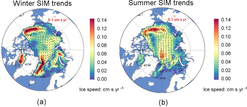
H. Bi et al.: Contributions of advection and melting processes to the decline in sea ice                                           1425

system (AMSR-E), to the International Arctic Buoy Pro-
gram (IABP) buoy data and surface winds from the Na-
tional Centers for Environmental Prediction and the National
Center for Atmospheric Research (NCEP/NCAR). The ver-
sion of the SIM product (v3.0) is available with a grid of
25 km × 25 km, and is mapped on an EASE-Grid projection,
which is an equal-area projection (Tschudi et al., 2019a, b).
The IABP buoy observations were employed throughout the
product with a few unrealistic buoys being removed due to er-
rors (Szanyi et al., 2016). Likewise, AVHRR imagery is used
for the period 1979–2000 with some error sources excluded.
Overall, the SIM data are estimated to have an uncertainty
of between 1 and 2 cm s−1 depending on the amplitudes of
both the sea ice concentration (SIC) and SIM (Sumata et al.,
2015). At the time this study was conducted, daily SIM data
from 1979 through 2016 were available. Note that the newest
version of the SIM product (Tschudi et al., 2019b) will soon
be released, based on which further analysis is expected.
   Satellite-derived daily SIC records (1978–2017) (http://          Figure 1. The fluxgate (red line) that is used to estimate sea ice
nsidc.org/data/NSIDC-0079, last access: 18 March 2019)               area flux. The blue lines represent the boundaries of the PA and AA
(Comiso, 2017) were also obtained from NSIDC. Common                 regimes. The endpoints in the North American and the Eurasian
with the SIM product, SIC is also extracted from multiple            sides are (125.1◦ W, 73.0◦ N) and (101.0◦ E, 79.6◦ N), respectively.
passive microwave observations from SMMR, SSM/I, and
SSMIS by the application of the bootstrap (BT) algorithm.
Over the period November 1978 to July 1987 the ice concen-           The length (km) of the chosen gate corresponds to the total
tration is available every other day. The data gap is filled us-     width of 113 grids. The monthly area flux (Fm ) is the sum
ing a temporal interpolation from the data of the two adjacent       of daily fluxes for the corresponding calendar month, and the
days (i.e., the previous and subsequent days). The concentra-        seasonal flux denotes the accumulative fluxes over the sum-
tion field utilized here is an up-to-date version (v3.1), offer-     mer (June–September) and winter (October–May) months.
ing improved consistency among the estimates from the dif-           Likewise, the annual flux is taken as the integrated flux over
ferent satellite observations through the application of vary-       annual cycles between October and September (i.e., the sum
ing tie points on a daily basis. Furthermore, the product is         of the winter and summer estimates). Although the focus sea-
optimized to further remove the effects of weather and land          son of this study is summer, the winter and annual fluxes
contamination (Cho et al., 1996). The data are available on a        across the gate are also presented for comparison to help
polar stereographic projection.                                      readers understand the relative contribution of summer ad-
                                                                     vection to the regional sea ice balance. We should note that
2.2   Procedure to estimate regional sea ice exchanges               the data quality for the daily SIC and SIM fields is likely
      and melt                                                       lower during summer due to the surface melting process.
                                                                        In our sign convention, sea ice transport from the PA to the
Following Kwok (2008a), the Arctic Ocean is divided into             AA sector is referred to as a positive flux (i.e., outflow) and
the PA and AA sectors (Fig. 1). The division is defined by a         the reverse direction is taken as a negative flux (i.e., inflow).
line linking the easternmost tip of Severnaya Zemlya and the         Supposing that the errors in the SIM grid samples are unbi-
southwestern tip of Banks Island. With a length of 2840 km,          ased, additive, uncorrelated, and normally distributed (Kwok,
the line serves as the gateway through which the sea ice area        2008b), the uncertainty of the daily fields can be expressed
flux between the two sides of the Arctic Ocean is calculated.        as follows.
   Sea ice area flux is taken as the integral product of gate-
                                                                          σd L
perpendicular SIM and SIC for all grids across the fluxgate.         σF = √ ,                                                        (2)
The daily field of sea ice area flux (F , km2 d−1 ) is written as           N
                                                                     where L represents the fluxgate width (2840 km), and σd is
      N−1
F=
      X
            ui ci 1x (i = 1, 2, . . ., N ),                   (1)    the uncertainty in the daily SIM. Regarding the daily drift
      i=1
                                                                     uncertainty for one ice sample (σd ), we use the uncertainty
                                                                     reported in Sumata et al. (2015), which is estimated by com-
where u, c, and 1x correspond to the gate-perpendicular              paring NSIDC SIM data with buoy drifts and varies on the
SIM (km d−1 ), SIC, and the width of a grid (25 km), and             basis of the magnitudes of SIC and SIM. The uncertainty
i = 1, 2, . . .N refers to the index of grid cells along the gate.   of the daily sea ice motion data during winter is obtained

www.the-cryosphere.net/13/1423/2019/                                                        The Cryosphere, 13, 1423–1439, 2019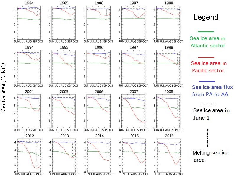
1426                                  H. Bi et al.: Contributions of advection and melting processes to the decline in sea ice

Table 1. Expected mean uncertainties in seasonal and annual sea    the Pacific sector is dominated by divergence over the ma-
ice area flux (106 km2 ).                                          jor parts (Lindsay et al., 2009), convergence may contribute
                                                                   to a percentage of no more than 1 %. This is much less than
        Length of     N    σsummer     σwinter   σannual           the estimated melting trend, approximately 3.2 % yr−1 for the
        fluxgate                                                   1979–2016 period as shown in Fig. 11. Based on these find-
        2840 km      113      0.004     0.005     0.007            ings, we ignore the limited contributions of convergence and
                                                                   divergence to sea ice area balance within the PA side.

                                                                   2.3     Large-scale atmospheric circulation index
as 2 cm s−1 (i.e., 1.70 km d−1 ) (Sumata et al., 2015). For the
summer period, however, the ice motion is often blurred by         The atmosphere circulation modes screened in this study
surface melting. Therefore, summer ice motion mainly relies        for possible linkages with sea ice area changes in PA in-
on interpolation that introduces additional uncertainty and        clude the AO (leading mode of sea level pressure (SLP)
thus has a poorer quality. As a result, we presumed summer-        north of 20◦ N) (Thompson and Wallace, 1998), NAO (lead-
period uncertainty to be twice the winter error, up to 4 cm s−1    ing mode of SLP over the North Atlantic) (Hurrell, 1995),
(i.e., 3.40 km d−1 ) in the fluxgate. Assessment for ice con-      and DA (the second-leading mode of SLP within the Arc-
centration fields show there is a uncertainty of 3 % in win-       tic Circle north of 70◦ N) (Wu et al., 2005). Both the AO
tertime consolidated ice areas, whereas it is estimated to be      and NAO indices (1979–2016) are available at the fol-
about 5–10 % in summer when melt-ponding effects play a            lowing sites affiliated with the Climate Prediction Center
role (Meier, 2005). In this study, we use 3 % and 10 % as the      (CPC) at the National Oceanic and Atmospheric Admin-
representative value of ice concentration uncertainties during     istration (NOAA): http://www.cpc.ncep.noaa.gov/products/
winter and summer periods, respectively (Meier, 2005).             precip/CWlink/daily_ao_index/ao.shtml (last access: 6 April
   The uncertainty of the seasonal (σsummer and σwinter ) or       2019) and http://www.cpc.ncep.noaa.gov/products/precip/
annual area flux estimates (σannual ) can be described as          CWlink/pna/nao_index.html (last access: 6 April 2019). The
         p                                                         DA corresponds to the second-leading mode of the empirical
σ = σF ND ,                                                  (3)
                                                                   orthogonal function (EOF) of monthly mean sea level pres-
where ND denotes the days for the period examined. Based           sure (SLP) north of 70◦ N during the winter season (October
on these equations, the expected uncertainties for the sea ice     to May; Wu et al., 2005). The SLP fields are obtained from
area flux estimates are obtained. The uncertainties listed in      the National Centers for Environmental Prediction (NCEP)
Table 1 correspond to 2.2 %, 1.4 %, and 1.2 % of the mean          and the National Center for Atmospheric Research (NCAR).
flux (as shown in Sect. 3.1.3) during summer, summer, and          The record of the DA index (1979–2016) was provided by
annual periods, respectively.                                      Bingyi Wu at Fudan University (personal communication,
   According to Kwok (2008a), the melting sea ice area in PA       2019).
is the difference between the total sea ice area loss in PA and
the sea ice area flux from PA to AA. A possible discrepancy        2.4     Arctic climate variables
is caused by deformation (divergence and convergence) pro-
                                                                   The changes in SLP can have significant impacts on winds
cesses, which can lead to reduction in sea ice area that may be
                                                                   and hence SIM through their perturbations of other cli-
misclassified as sea ice loss due to melt or export. The coarse
                                                                   mate variables, such as surface air temperature (SAT) and
resolution of satellite observations does not allow us to ac-
                                                                   precipitable water (PW). All these data are obtained from
curately quantify the sea ice loss in relation to sea ice defor-
                                                                   NCEP/NCAR in NOAA (Kalnay et al., 1996), with a grid
mation. However, in winter, sea ice area change due to defor-
                                                                   size of 2.5◦ × 2.5◦ .
mation is expected to be negligible due to solid pack ice (ap-
proximately 1 %–2 %) (Kwok et al., 1999). In summer, the
deformation may be larger. A larger (smaller) convergence          3     Results
(divergence) is hypothesized north (south) of 80◦ N. For ex-
ample, the accumulated divergence south (north) of 80◦ N           3.1     Sea ice transport between the Pacific-Arctic and
is approximately 14 % (25 %) in 2007 (Kwok and Cunning-                    Atlantic-Arctic oceans
ham, 2012). The PA sector is an area located mostly south of
80◦ N where ice divergence is more likely to occur in sum-         3.1.1    Comparison with a previous estimate
mer, and new ice likely does not form within the divergence
area due to warm temperature. In this study, it is difficult to    To give credence to our estimates, we compared the estimates
quantitatively separate the ice loss due to deformation from       with the results reported by Kwok (2008b). He made use
the melting process. However, a sophisticated model study          of the SIM data retrieved from the 37 GHz channels of the
(Lindsay et al., 2009) suggests the convergence accounts for       combined 29-year SMMR and SSM/I time series between
1 % of the Arctic basin ice loss in the Atlantic sector. Since     1979 and 2007. Overall, the two estimates agree well with

The Cryosphere, 13, 1423–1439, 2019                                                     www.the-cryosphere.net/13/1423/2019/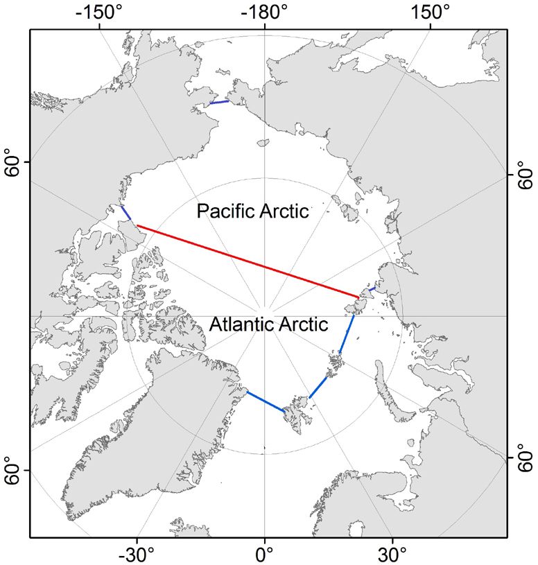
H. Bi et al.: Contributions of advection and melting processes to the decline in sea ice                                               1427

Figure 2. Comparison of regional sea ice exchanges between the PA and AA sectors in (a) summer and (b) winter. Our estimates are
compared with a previous 29-year record (1979–2007) provided by Kwok (2008b). The dashed line is the linear fit line between the two
estimates. The solid line denotes the “Y = X” line. The linear relationship equation and correlation coefficient (R) between the two records,
as well as the mean bias and standard deviation (SD) of the difference, are also displayed.

respect to summer and winter sea ice area fluxes (Fig. 2).               yet almost all months experience positive ice flow anoma-
As shown in Fig. 2, data pairs are distributed close to the              lies in 1995, 2007, and 2008. The frequently observed posi-
Y = X line. There is a small mean positive bias between                  tive anomaly in recent periods compared to the early period
the two estimates, with Kwok’s estimates slightly larger than            (1979–1987) is further reflected in the annual mean normal-
ours, approximately 0.015 × 10⁶ km2 in summer (Fig. 2a)                  ized anomaly (bottom row in Fig. 3).
and 0.028 × 10⁶ km2 in winter (Fig. 2b). These biases cor-                  The temporal variability in the monthly sea ice area flux
respond to 8.6 % and 8.2 % of the mean estimates of sea                  fields is further emphasized in Fig. 4, where the frequency
ice area flux (as shown below in Sect. 3.1.3) during summer              distribution histogram for months with different normal-
(0.173 × 10⁶ km2 ) and winter (0.337 × 10⁶ km2 ) seasons, re-            ized anomaly amplitudes are displayed for different decades
spectively. Moreover, a good consistency in terms of interan-            (P1: 1979–1988; P2: 1989–1998; P3: 1999–2008, P4: 2009–
nual variability is identified as indicated by high correlation          2016). The dominance of anomalous low sea ice area fluxes
coefficients (R = 0.91 in summer and R = 0.96 in winter).                during the first decade is reflected as an asymmetric distri-
                                                                         bution pattern in frequency (Fig. 4a), with a larger number
3.1.2    Monthly sea ice area flux                                       of months decreasing to the negative anomaly side. Compar-
                                                                         atively, for the following three periods (Fig. 4b–d), the dis-
The normalized monthly anomaly data have been adopted                    tribution pattern begins to become more symmetric, mainly
for studying the monthly variability. As a result, the seasonal          because of the growing number of months with positive
variability is removed and, therefore, the distinct variations           anomaly fields.
in monthly estimates are clearer and a direct comparison                    To depict the decadal evolution in frequency distribution,
of variability among different months is feasible. The nor-              the individual months for each period are binned into four
malized or standardized procedure applied for the monthly                groups with different anomaly amplitude ranges (A ≤ −1,
anomaly fields (Fa ) can be written as                                   −1 < A ≤ −0.5, 0.5 < A ≤ 1, A > 1) and shown as inset
                                                                         text in Fig. 4. The fraction is the ratio between the number
        Fm − Fm0
Fa =             ,                                              (4)      of months affiliated with a specific range and the number
          σFm                                                            of all months of the corresponding decadal period. In this
                                                                         case, there are 120 months for each of the first 3 decades and
where Fm represents monthly area flux and Fm0 and σFm in-
                                                                         96 months for the last. Specifically, during the first decade
dicate the means and standard deviations (SDs) of the cor-
                                                                         (P1) approximately 43 % of the months have normalized
responding month over the investigated period (1979–2016),
                                                                         anomaly values less than −0.5, in contrast to only 15 % of
respectively, and the results are shown in Fig. 3.
                                                                         the months showing positive normalized values of greater
   Figure 3 displays the variations in anomaly fields for
                                                                         than 0.5 (Fig. 4a). In comparison, during the following three
monthly sea ice flux between the two subsectors in the Arctic
                                                                         periods (Fig. 4b–d), the fractions of months with signif-
Ocean. Overall, the temporal variability is high (Fig. 3). The
                                                                         icant negative normalized anomaly values less than −0.5
first decade (1979–1988) is characterized by the occurrence
                                                                         (−1 < A ≤ −0.5 and A ≤ −1) plummet to less than 28 %,
of frequent negative anomaly fields, while for the remain-
                                                                         but 24 %–30 % of the months are observed to have a dis-
ing periods the emergence of positive anomalies seems to be
                                                                         tinct positive anomaly value at least of 0.5 (i.e., 0.5 < A ≤ 1
more common (Fig. 3). In particular, negative anomalies are
                                                                         and A > 1). In addition, the fraction changes for the extreme
observed in nearly all months (except for February) in 1985,

www.the-cryosphere.net/13/1423/2019/                                                            The Cryosphere, 13, 1423–1439, 2019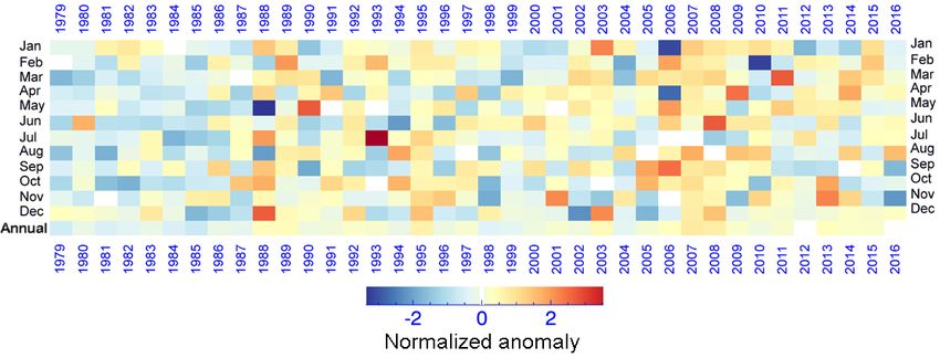
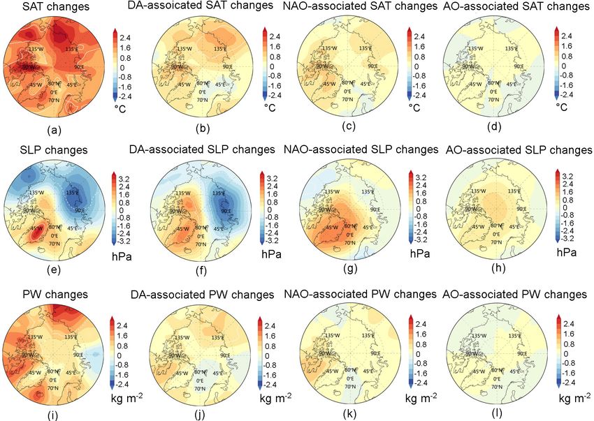
1428                                   H. Bi et al.: Contributions of advection and melting processes to the decline in sea ice

Figure 3. Normalized monthly anomaly fields of sea ice area flux. The anomaly field is calculated as the difference between the monthly
estimate and the mean value of the same month computed over the period of interest. Then, the normalized anomaly field is obtained by
dividing the monthly anomaly field by the standard deviation (SD) of the corresponding month over the 38-year period. The bottom row
denotes the annual mean value of the normalized anomaly.

Figure 4. Frequency distribution histograms for months with different normalized anomalies in sea ice area flux in different decades. The
fraction depicted as the percentage for each period, for example, (0.5 < A ≤1) = 7.5 % as presented in panel (a), refers to the ratio between
the frequency of the months sorted into the outlined range and the total number of months during the examined decades.

cases (|A| ≥ 1) remain relatively steady with time, varying              mean value of 2.52 % yr−1 . The largest trend appears in Au-
between 26 % and 29 %. However, the extreme low anoma-                   gust (11.6 % yr−1 , significant at the 90 % level), whereas the
lies (A ≤ −1) decrease from 20.8 % in P1 to 10.4 %, while                lowest occurs in January (−3.67 % yr−1 , not statistically sig-
the extreme high anomalies (A > 1) increase from 7.5 % to                nificant). The positive trend in August is mainly associated
16.6 %. This shift in sea ice exchanges between the PA and               with an increasing trend in SIM in the transpolar drift stream
the AA sectors may indicate a shift of atmospheric circula-              (Fig. 5a). The negative trend in January is linked to the trend
tion toward a pattern facilitating sea ice export out of the PA          pattern from the Laptev Sea through the central Arctic to the
side (Wu et al., 2005; Zhang et al., 2008; Jia et al., 2009)             east of the Beaufort Sea (Fig. 5b). The changes in SIM ex-
   The monthly trends in the sea ice area flux are listed in             plain a major part (R 2 = 0.98) of the trends and variability in
Table 2. The trend in percentage for each month denotes the              sea ice area flux (Fm ), and the remaining minor part is deter-
fraction of the monthly trend estimate relative to the mean              mined by the SIC changes, which induce negative contribu-
sea ice area flux for the corresponding month. Basically, all            tions to the monthly flux trends during summer but small pos-
months (except for January) show positive trends, with a

The Cryosphere, 13, 1423–1439, 2019                                                            www.the-cryosphere.net/13/1423/2019/

H. Bi et al.: Contributions of advection and melting processes to the decline in sea ice                                                                   1429

Figure 5. Sea ice motion trend in (a) January and (b) August. The magnitude of ice motion is indicated by background color and the length
of arrows.

Table 2. Monthly trends for the sea ice area flux between PA and AA. The trends for the SIM and SIC fields over the fluxgate are also
provided (% yr−1 ).

                    Jan        Feb         Mar         Apr           May           Jun        Jul       Aug          Sep        Oct        Nov       Dec
        Fm      −3.67        0.07       5.28∗∗       3.27∗        2.68∗         1.53∗      1.17       11.6∗       1.77       4.32∗        1.77      0.43
        SIM     −3.66        0.35       5.49∗∗       3.67∗        2.94∗         2.04∗      0.53      10.44∗       2.23       3.95∗        2.47      1.20
        SIC     0.007       0.016        0.010       0.009       −0.033        −0.072    −0.165      −0.531     −0.650      −0.183      −0.002     0.012

    Note: ∗ and ∗∗ denote the significance level at 95 % and 99 %, respectively.

itive contributions during winter months (December to April)
(Table 2).

3.1.3    Annual and seasonal sea ice area flux

Figure 6 shows the estimates of the sea ice area transport
for different seasons and years between the two sectors. The
average annual sea ice export of 0.51(±0.314) × 106 km2
comprises the mean winter and summer contributions of
0.337(±0.263) × 106 km2 (or 66 %) and 0.173(±0.153) ×
106 km2 (or 34 %), respectively. The number after the sign
“±” denotes the standard deviation of 38-year sea ice area
flux. Annually, sea ice area flux peaked at 1.089 × 10⁶ km2
in 2007/2008 and set a record low of −0.107 × 10⁶ km2 in
1984/1985. Seasonally, the winter sea ice exports vary be-                               Figure 6. Annual and seasonal sea ice area fluxes between the PA
tween −0.152 × 10⁶ km2 (1998/1999) and 0.848 × 10⁶ km2                                   and AA sectors over the period 1979–2016. The annual ice flow (an-
                                                                                         nual cycle) is shown by the green line. Summer (from June through
(2013/2014), whereas the summer ice flux fluctuates within
                                                                                         September) and winter (from October through May) fluxes are de-
a range from −0.166 × 10⁶ km2 (1981) to 0.559 × 10⁶ km2                                  noted with blue and red lines, respectively. The dashed lines repre-
(2006). The negative (positive) sea ice area flux as mentioned                           senting the linearly fitted trends are obtained through the application
above points to a net sea ice inflow (outflow) from the AA to                            of the least-squares method. The labels ∗ , ∗∗ , and ∗∗∗ correspond to
PA side (from the PA to AA side).                                                        the significance at the levels of 90 %, 95 %, and 99 %, respectively.
   Over the 38-year period, significant positive trends are ob-
served for the sea ice area fluxes during the summer and win-
ter seasons (Fig. 6). Over the 38-year period, the winter sea                            tribute to an upward trend in annual sea ice area flux of
ice export exhibits a positive trend of 0.009 × 10⁶ km2 yr−1                             0.013 × 10⁶ km2 yr−1 (i.e., 2.61 % yr−1 , significant at a 99 %
(i.e., 2.72 % yr−1 , significant at a 95 % level), and the sum-                          level). The trend within the parentheses, expressed as per-
mer export increases at a rate of 0.004 × 10³ km2 yr−1 (i.e.,                            centage per year, is taken by dividing the trend estimate by
2.40 % yr−1 , significant at a 90 % level). Together, they con-                          the corresponding 38-year mean estimate of sea ice area flux.

www.the-cryosphere.net/13/1423/2019/                                                                             The Cryosphere, 13, 1423–1439, 2019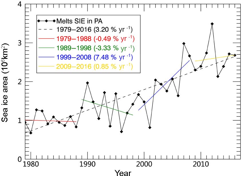
1430                                 H. Bi et al.: Contributions of advection and melting processes to the decline in sea ice

The sharp increase since 1989 and onward for the winter ex-        ing summer scarcely changed before 2008 (the first three
port (Fig. 6), in contrast to the preceding period 1979–1988,      rows in Fig. 9). AA is located at higher latitudes where less
preconditions for a significant positive trend in the winter as    melting is expected compared the PA. However, recent sea
well as annual fields of outflow. Nonetheless, the summer          ice area changes reveal a shrinkage of sea ice area approx-
ice area flux features a gradual increase over the whole pe-       imately 0.28 × 10⁶ km2 within the AA sector in September
riod, with anomalously large ice export occurring between          2012 to 2013 (Fig. 9). The sea ice loss within the AA may be
2006 and 2010 (approximately 0.310×10⁶ km2 , on average),          more evident if the starting date of melting becomes earlier
which is favorable for the maintenance of the overall positive     (Stroeve et al., 2014) and melting intensity is reinforced by
trend in summer.                                                   the positive feedback mechanism of ice albedo (Perovich et
   Due to the extensive coverage in longitudes and latitudes       al., 2007, 2008; Screen and Simmonds, 2010) and/or if sea
across the investigated fluxgate (2840 km), regional varia-        ice outflow through the Fram Strait is enhanced (Kwok et al.,
tions in the trend of the across-gate sea ice area flux fields     2013; Bi et al., 2016; Smedsrud et al., 2017).
are expected. Broadly, the Arctic sea ice circulation is char-        With the sea ice area budget shown in Fig. 9, we quan-
acterized by the Beaufort Gyre (BG) and transpolar drift           tify the relative contribution to sea ice area changes in sum-
stream (TDS). How does the SIM trend vary in these two             mer due to the advection and melting processes over the
regimes? To answer this question, we not only present the          period of 1979–2016 (i.e., melting (M) = observed area
overall pattern of spatial distribution of SIM trends over the     change (O) − advection (A)). As a fractional contribution,
entire Arctic Ocean (Fig. 7), but also depict the details of       the advection and melting processes, on average, account for
the cross-gate SIM trends in fields (Fig. 8). Figure 7 shows       9.6 % (i.e., A/O × 100 %) and 90.4 % (i.e., M/O × 100 % or
that SIM increases in the BG and TDS regimes during both           (A − O)/O × 100 %), respectively, of the observed ice area
winter (Fig. 7a) and summer (Fig. 7b) seasons. In particu-         loss within the PA sector during summer months. Interannual
lar, the increasing SIM trends in the narrow southern arm          variability in fractions is distinct, as suggested by the stan-
of the BG regime appear in winter (Fig. 7a) and summer             dard deviation of approximately 9 %. However, no significant
(Fig. 7b) The SIM trends during winter (summer) of approx-         trend is identified in the fractions of sea ice area in connec-
imately 0.12 cm s−1 yr−1 (0.11 cm s−1 yr−1 ) (i.e., approxi-       tion with the two processes (Fig. 10). The smallest (largest)
mately 0.10 km yr−1 ) over the southern arm of the BG lead         fraction of 72.6 % (110.2 %) in the sea ice area change due to
to a reduced net sea ice export (i.e., more ice inflow) through    melting was observed in 2006 (1979), along with the largest
the west end of the fluxgate (Fig. 8a and b). The increasing       (smallest) fraction of 27.4 % (−10.2 %) due to sea ice area
SIM in the TDS is 0.07 cm s−1 yr−1 (0.04 cm s−1 yr−1 ) (i.e.,      advection (Fig. 10). The negative fraction with respect to ad-
approximately 0.06 km yr−1 (0.03 km yr−1 )) during the win-        vection suggests a net inflow from the AA to PA side. In this
ter (summer) season. Therefore, increasing sea ice outflow         case, the actual melting area (O − A) is thus larger than the
through the TDS is compensated for by sea ice inflow asso-         directly observed area changes (O), causing a melting frac-
ciated with the BG. Compared with that in winter (Figs. 7a         tion greater than 100 %. Over the examined period, the cases
or 8a), the sea ice trend in the TDS (Figs. 7b and 8b) shifts      with a net increase in advective ice area took place before
its central axis to parallel to the prime meridian. Overall,       1985.
the SIM trend pattern appears to form an Arctic-wide anti-            The trend of melting sea ice area within the PA is ap-
cyclonic mode. As discussed below, this mode has crucial           parent over the 38-year period (Fig. 11), with an overall
meanings for the retreat of sea ice in the Pacific sector during   positive trend of 3.20 % yr−1 (significant at the 99 % level)
summer.                                                            (Fig. 11). Since the mid 1990s, sea ice melting within the
                                                                   PA has been continually enhanced (Fig. 11), which is associ-
3.2    Melting sea ice within the Pacific sector in summer         ated with Arctic amplification (Screen and Simmonds, 2010).
                                                                   Decadal variability is also significant. The greatest increase
Sea ice melting is a sensitive indicator reflecting the warmer     of 7.48 % yr−1 (significant at the 99 % level) occurred in the
Arctic climate. An estimate of melting area of sea ice             third decade (1999–2008), whereas the remaining 3 decades
(dotted–dashed line in Fig. 9) is obtained as the difference       show moderate or even negative trends.
between the observed sea ice area loss in the PA (red line in         Additionally, note that the day of year (DOY) of the min-
Fig. 9) and the sea ice area flux through the fluxgate (blue       imum sea ice area in the PA sector displays an overall posi-
line in Fig. 9) during the summer season (June–September).         tive trend of 0.29 d yr−1 (Fig. 12). The trend implies a grad-
Over the 38-year period, the mean melting area is 1.66 ×           ually delayed occurrence of the DOY of the minimum sea
106 km2 , with a distinct variation from 0.68×10⁶ km2 (1980)       ice area in the PA. There are also decadal variations in this
to 3.49 × 10⁶ km2 (2012). Noticeably, the PA sector seems          DOY. In particular, over the second (1989–1998) and third
to have been shifted into a new era from 2007 onward, with         decades (1999–2008), the trends in DOY approach approxi-
large ice melting of 2.70×10⁶ km2 yr−1 during the post-2007        mately 1.46 and 1.63 d yr−1 , respectively (Fig. 12). The over-
period compared with 1.70 × 10⁶ km2 yr−1 for the period be-        due DOY is associated with the earlier beginning of the melt-
fore 2007. In contrast, the sea ice area in the AA sector dur-     ing date (Stroeve et al., 2014) and the positive sea ice albedo

The Cryosphere, 13, 1423–1439, 2019                                                    www.the-cryosphere.net/13/1423/2019/
H. Bi et al.: Contributions of advection and melting processes to the decline in sea ice                                             1431

Figure 7. SIM trends during (a) winter (October–May) and (b) summer (June–September) over the period 1978/1979–2015/2016 and 1979–
2016, respectively.

Figure 8. Cross-gate SIM climatology (black solid line) and trends (arrows) for (a) winter and (b) summer over the 38-year period. The left
end represents for the North American side and the right the Eurasian side.

feedback loop (Perovich et al., 2008), which allows more                et al., 2017). The Arctic-wide wind forcing is linked to large-
heat to be absorbed in the area of ice loss, facilitates more           scale atmospheric circulation patterns (Zhang et al., 2008;
melting of sea ice in the PA sector, and results in later oc-           Overland and Wang, 2010; Stroeve et al., 2011). Hence, the
currence of the minimum sea ice area. However, since 2009,              connection between the sea ice area loss in the PA sector
the DOYs appear to have recovered to the former state in the            and three typical atmospheric indices (AO, NAO, and DA)
1980s (Fig. 12). This reversion can be explained by the with-           is assessed here. NAO and AO represent the dominant atmo-
drawal of the sea ice extent toward a position farther north            spheric circulation modes in guiding sea ice movement and
at high latitudes (Figs. 9 and 11), where freezing usually              Fram Strait export before 1994 (Rigor et al., 2002; Naka-
starts earlier in comparison with areas at southern latitudes           mura et al., 2015), while the DA seems to play a leading role
(Stroeve et al., 2014).                                                 over the latter period after 1995 (Wang et al., 2005). Here
                                                                        our objective is to examine how the sea ice variability due
                                                                        to advection and melting processes is quantitatively related
4   Discussion                                                          to the interannual and decadal changes in these atmospheric
                                                                        modes. Furthermore, the potential impacts on sea ice loss in
Wind forcing has been significant in modulating the sea ice             related climatic variables (SAT, SLP, and PW) coupled with
variability in summer (Ogi et al., 2016). As an example, sea            different atmospheric circulation patterns are highlighted.
ice depletion induced by the summer melting process is con-                Overall, the interannual variability for the three indices
nected to the wind forcing, which can help to cause a warmer            is large, and two indices, NAO and DA, reveal significant
Arctic climate through the advection of warmer and moister              trends during summer (Fig. 13). Over the investigated 38-
air from the south (Wang et al., 2005; Zhang et al., 2013; Lee          year period, the sea ice area reduction in summer within the

www.the-cryosphere.net/13/1423/2019/                                                           The Cryosphere, 13, 1423–1439, 2019
1432                                    H. Bi et al.: Contributions of advection and melting processes to the decline in sea ice

Figure 9. Selected daily changes in sea ice areas within the PA (red) and AA (green) during summer (June–September) for the period 1979–
2016. The horizontal dashed line represents the sea ice area in the PA on 1 June, which is used as a benchmark to measure the sea ice area
changes due to melting. The cumulative daily sea ice area flux, with reference to the top dashed line, is shown as a blue line. The melting sea
ice area, denoted by the vertical dotted–dashed line, is taken as the difference between the total decline in sea ice area within the PA and the
accumulated flux through the gate.

Figure 10. Fractions of sea ice area loss in the PA sector that are
related to the sea ice melting and advection processes.

                                                                          Figure 11. Time series for melting sea ice areas within PA.
PA seems to have been slightly influenced by AO fluctua-
tions, with a low correlation coefficient (R) of −0.24 (Ta-
ble 3). Separately, the sea ice area variations caused by ad-             NAO and DA, which show relatively strong correlations with
vection and melting are barely attributable to the AO effects             the changes in sea ice area in the PA (Table 3).
(Table 3). Therefore, in the following, we focus our analysis
on the effects of the atmospheric circulations associated with

The Cryosphere, 13, 1423–1439, 2019                                                              www.the-cryosphere.net/13/1423/2019/
H. Bi et al.: Contributions of advection and melting processes to the decline in sea ice 1433
observed (Kwok, 2008a). The moderate negative correlation
between NAO and melting sea ice area (R = −0.47) corrob-
orates this hypothesis.
The overall association between sea ice area variabil-
ity and the DA index is comparatively robust (R = 0.63).
Considering the clear positive trend in DA (1979–2016)
(Fig. 13c), the SLP changes explained by the DA trend
are characterized by a dipole pattern with one action cen-
ter over the Barents and Laptev seas and the other center
of action appearing on the opposite side over the Canadian
Archipelago and Greenland (Fig. 14f). In fact, the spatial dis-
tribution for the DA-associated SLP changes over the Arc-
tic basin is broadly consistent with those for the actual SLP
changes (Fig. 14e), except for a prominent negative SLP cen-
ter over the North Pacific and an enhanced positive SLP cen-
Figure 12. Day of year (DOY) of the annual minimum sea ice area
ter over Greenland. With this type of SLP distribution, the
in PA. DA-associated winds induce strengthened meridional ice ad-
vection through the TDS within the central Arctic (Figs. 5, 6b
in Sect. 3.1.3). A more rapid transpolar advection of sea ice is
Table 3. Correlations between summer mean atmospheric index and
thus responsible for the observed increasing trend in the sea
total sea ice area loss, and sea ice area decline due to melting and
ice outflow from the PA to the AA sectors (Fig. 7b). In addi-
advection processes over the period 1979–2016.
tion, with such DA-associated SLP changes, more warmer air
Atmospheric Melting Net sea ice Total ice retreat
from the southern areas can be advected into and warm the
index sea ice advection (melting + SAT in the northern Arctic, finally augmenting the ice melt-
(summer mean) advection) ing process (Zhang et al., 2013; Lee et al., 2017). Indeed,
an SAT ridge centered on the East Siberian Sea is observed
AO −0.28 0.14 −0.24 (Fig. 14b). As a response, the cold air of the high-latitude
NAO −0.47 −0.18 −0.46
Arctic origin is pushed out toward the southern areas, reduc-
DA 0.55 0.74 0.63
ing the local SAT over the eastern Greenland Sea, Barents
Sea, and Kara Sea regions (Fig. 14b).
Associated with the DA-associated SLP distribution pat-
The influence of NAO-associated atmospheric circulation tern, the emergence of enhanced BG circulation is identified
in winter on sea ice changes in summer has been broadly in the Beaufort Sea (Fig. 14f). In particular, the sea ice drifts
documented (Kwok, 2000; Jung and Hilmer, 2001; Parkin- in the southern arm of the BG regime are largely strength-
son, 2008), which is especially clear for the period from the ened (Fig. 7b), which contributes to the large inflow of sea
late 1980s to early 1990s (Jung and Hilmer, 2001) when NAO ice to the southern Beaufort Sea (Fig. 8b), where sea ice un-
was in its peak positive phase. In this study, the summer NAO dergoes dramatic melting processes in summer as indicated
is negatively correlated with the summer retreat of sea ice by the remarkable SAT increase there (Fig. 14a). This cou-
area within the PA sector (R = −0.46) over the 38-year pe- pled mechanism between dynamic (advection) and thermo-
riod. Table 2 shows a stronger connection with the sea ice dynamic (melting) processes resembles that caused by the
area change due to melting (R = −0.47) than with the sea NAO. As a consequence, the depletions in sea ice in summer
ice area loss in relation to advection (R = −0.18). That is, a due to both melting and advection are relatively strongly cor-
negative NAO in summer would favor more sea ice melting related to the DA index of summer, with R values of 0.55 and
and hence less ice coverage. 0.74, respectively, over the entire period (Table 3).
As there is a clear negative trend in the summer mean NAO Since AO shows a negligible trend (Fig. 13a), the 38-year
index (Fig. 13b), one may wonder how the summer NAO in- climatic changes related to AO are insignificant (Fig. 14d,
dex trend is related to the increasing loss of sea ice within the h, and i) and smaller in magnitude compared to the DA-
PA sector. As shown in Fig. 14g, the NAO-associated SLP and NAO-associated changes. The NAO pattern is conven-
distribution pattern, with a greater SLP in the western Arc- tionally deemed a regional index, representing parts of the
tic near the Canadian Archipelago, is favorable for a pattern broader AO pattern. However, NAO-associated SLP changes
of anticyclonic atmospheric circulation within the PA. Such (Fig. 14g) show a stronger gradient across the fluxgate than
a clockwise pattern of atmospheric circulation is hypothe- that of AO-associated SLP (Fig. 14h), which would favor
sized to push more ice from the eastern and northern Beau- more sea ice outflow from the PA to AA sectors. In compar-
fort Sea to the western and southern Chukchi Sea (Figs. 7b ison with NAO (Fig. 14g), the AO-associated SLP distribu-
and 8b), where extensive sea ice melting has been commonly tion shows a much weaker gradient across the Arctic Ocean
www.the-cryosphere.net/13/1423/2019/ The Cryosphere, 13, 1423–1439, 20191434 H. Bi et al.: Contributions of advection and melting processes to the decline in sea ice
Figure 13. Variations in and trends of the mean atmospheric indices in summer (June–September), including (a) the AO, (b) the NAO, and
(c) the DA index. The linear trends of NAO and DA indices are both significant at the 95 % significance levels according to the t-test method,
while the AO index reveals an insignificant trend.
Table 4. Correlations between summer mean atmospheric index and sea ice minimum area in the PA sector for the different decades and the
whole 38-year period.
Summer P1 P2 P3 P4 Overall
(Jun–Sep) 1979–1988 1989–1998 1999–2008 2009–2016 1979–2016
AO 0.57 0.46 0.39 −0.34 0.24
DA −0.03 −0.16 −0.68 −0.45 −0.63
NAO 0.16 0.24 0.23 0.87 0.46
(Fig. 14h), although it may contribute to the sea ice advection clear and decreasing positive effects over the first 3 decades
from the Pacific side to the Atlantic side. As a result, lower but reversing to a negative moderate impact in the last period
correlations between AO and sea ice melting and advection (P4) (Table 4). A clear association with DA arises during the
processes are expected, with R = −0.28 and 0.14 (Table 3). latter two periods: P3 (1999–2008) and P4 (2009–2016). In
However, these small overall correlations do not necessarily contrast, the NAO index appears to have a significant impact
imply that AO plays no role in causing sea ice variations. only during the last period (2009–2016) (Table 4).
For instance, throughout the examined periods, AO exerted PW serves as an important indicator of Arctic climatic
more influences on sea ice changes for the earlier 2 decades conditions. In view of the distribution of PW changes
(1979–1998), with R = 0.57 and 0.46 (Table 4). (Fig. 14i), we find it broadly agrees with that of SAT in
The temporally varying association between atmospheric the PA sector (Fig. 14a). For example, over the Siberian
circulation and sea ice drift reflects Arctic climate changes. marginal seas, warmer SATs accompany more PWs. If the
How does the linkage vary with time? Does it remain sta- PW constituents drop to the surface as rain during a warming
ble? To answer these questions, correlations between differ- summer, they may benefit the melting process of the local
ent summer mean atmospheric indices and minimum sea ice ice/snow surface by lowering the surface albedo of ice/snow.
areas in the PA sector over different decades are obtained Compared with the NAO-associated changes (Fig. 14k), the
(Table 4). The AO effects are relatively unstable, imposing spatial distributions of DA-associated SAT (Fig. 14b) and
The Cryosphere, 13, 1423–1439, 2019 www.the-cryosphere.net/13/1423/2019/H. Bi et al.: Contributions of advection and melting processes to the decline in sea ice 1435
Figure 14. The changes in typical climate variables (SAT, SLP, and PW) over the 1979–2016 period (the first column, panels a, e, and i).
The change is obtained by multiplying the trend estimate (regression map) and the time span of the period (i.e., 38 years). The regressions
of these climatic variables on the DA (the second column, panels b, f, and j), NAO (the third column, panels c, g, and k), and AO (the fourth
column, panels d, h, and l) are also presented.
PW changes (Fig. 14j) are, to a greater degree, consistent
with those of the summer SIC trends (Fig. 15), particularly
over the area throughout the marginal seas in the PA sector,
such as the Beaufort Sea, Chukchi Sea, East Siberian Sea,
and Laptev Sea where the rates of sea ice area decline ap-
proach 2.0 % yr−1 . Conversely, we note that the magnitudes
of SAT (or PW) changes in connection with the DA and NAO
are far less comparable to the total SAT (or PW) changes, and
similarity in spatial distribution between Fig. 14b and c (or
Fig. 14j and k) is not readily identifiable. This result occurs
because, aside from the effects of atmospheric circulation,
other mechanisms also play important roles in the large and Figure 15. Summer SIC trends over the period 1979–2016.
broad increases in SAT and thus PW over the Arctic, such
as the sea ice albedo feedback loop, the intrusion of warmer
Pacific-Atlantic Ocean water (Shimada et al., 2006; Tverberg
et al., 2014; Alexeev et al., 2017), cloud feedback (Liu et al., To summarize this section, we found different atmospheric
2008; Schweiger et al., 2008), and the changes in strength of forcing patterns exert varying influences on summer sea ice
the Atlantic meridional overturning current (AMOC) (Chen variability. Overall, the connections are relatively strong be-
and Tung, 2018). tween sea ice loss and DA (R = 0.63) and NAO (−0.46),
but fragile with AO (R = −0.24). In particular, the DA af-
www.the-cryosphere.net/13/1423/2019/ The Cryosphere, 13, 1423–1439, 20191436 H. Bi et al.: Contributions of advection and melting processes to the decline in sea ice
fects sea ice loss through both advection (R = 0.74) and polar stream, leading to increased sea ice outflow and more
melting (R = 0.55) processes, whereas the NAO acts promi- ice decline in the PA. Thermodynamically, both the DA and
nently on the melting process (R = −0.46). This is consis- NAO indices are associated with a strengthened anticyclonic
tent with previous arguments that the DA plays a more vi- SLP pattern over the southern Beaufort Sea. This feature will
tal role in promoting summer sea ice depletion (Jia et al., promote the westward transport of sea ice from the Cana-
2009). Furthermore, our analysis shows that the connections dian Basin to the south of the Beaufort Sea and Chukchi Sea
are not invariant on a decadal scale, but are characteristic where extensive melting sea ice has been detected in sum-
with a regime shift (Table 4). Accordingly, the linkage be- mers during the recent decade. By contrast, AO-associated
tween atmospheric forcing and sea ice loss is stronger during sea ice changes due to melting and advection processes are
the earlier 2 decades (1979–1998) with AO and NAO, but not distinct, although temporally robust correlation is ex-
more robust with DA for the latter 2 decades (1999–2016). pected (Table 4).
Since DA is becoming a more favorable pattern for summer The significant sea ice retreat also plays a crucial role in
sea ice loss through both dynamic and thermodynamic forc- triggering regional responsive feedback in the atmosphere
ing, the causes for its surface emergence and amplification (Overland and Wang, 2010), as indicated by the warmer SAT
remain unclear and need further investigation. (Fig. 13a) and decreased SLP (Fig. 13d) observed on the
broad Siberian Arctic Ocean side. Therefore, if the current
distinct sea ice loss on the Pacific-Arctic Ocean persists, the
5 Concluding remarks diminishing SLP in areas over the Laptev Sea, one of the cen-
ters of action of the DA, will further enhance the positive DA
Using the new version (v3.0) of NSIDC products (SIM and trend. Consequently, stronger dynamic (advection) and ther-
SIC), we quantify the contributions of the advection and modynamic (melting) effects associated with the DA on sea
melting processes to the sea ice retreat within the PA sec- ice retreat within the PA sector are probably foreseen in the
tor over the period 1979–2016. A synoptic view of their predictable future.
38-year variability and trends on different timescales is pre-
sented. Over this period, the annual (October to following
September) mean sea ice export is 0.510(±0.314)×106 km2 , Data availability. NSIDC sea ice motion is available at
with summer (June–September) and winter (October–May) http://nsidc.org/data/NSIDC-0116 (Tschudi et al., 2019a). NSIDC
outflows of 0.173 × 10⁶ km2 (or 34 %) and 0.337 × 10⁶ km2 sea ice concentration employed to calculate sea ice area flux is
(or 66 %), respectively. A positive trend for the annual available at http://nsidc.org/data/NSIDC-0079 (Comiso, 2017).
The reanalysis data of SLP, SAT, and PW are available at https:
sea ice outflow is also identified, at approximately 0.013 ×
//www.esrl.noaa.gov/psd/cgi-bin/db_search/DBListFiles.pl?did=
106 km2 yr−1 (or 2.08 % yr−1 ), which is attributable to the
195&tid=72450&vid=676, https://www.esrl.noaa.gov/psd/cgi-bin/
increasing export of 0.009 × 10⁶ km2 yr−1 (or 2.72 % yr−1 ) db_search/DBListFiles.pl?did=195&tid=72451&vid=3083, and
in winter and increasing outflow of 0.004 × 10⁶ km2 yr−1 (or https://www.esrl.noaa.gov/psd/cgi-bin/db_search/DBListFiles.pl?
2.43 % yr−1 ) in summer. At the same period, sea ice area did=195&tid=73261&vid=1848, respectively (Kalnay, 2019a, b,
loss linked to the melting in summer, on average, amounts to c). Climatic variables AO and NAO are available at http://www.cpc.
1.66 × 10⁶ km2 , with a significant positive trend of 0.053 × ncep.noaa.gov/products/precip/CWlink/daily_ao_index/ao.shtml
106 km2 yr−1 (3.20 % yr−1 ). Further, we examine the relative (Thompson and Wallace, 2019), and http://www.cpc.ncep.noaa.
roles of ice advection and melting in the decline of sea ice gov/products/precip/CWlink/pna/nao_index.html (Hurrell, 2019).
within the PA where dramatic sea ice retreat has occurred in
summer during recent years. As a percentage, the sea ice de-
pletions in the PA due to the advection and melting processes Author contributions. HB and QY led the analysis and integrated
account for 9.6 % and 90.4 %, respectively. the data. XL, LZ, YW, and YL process the sea ice motion and sea
ice concentration data. HB, XL, and LZ performed the area flux cal-
The linkage between sea ice loss and wind forcing associ-
culations. HB, QY, and HH drafted the paper. All authors discussed
ated with different large-scale atmospheric circulations dur-
the results and commented on the paper.
ing the summer season is explored. Overall, the AO is weakly
connected to the sea ice loss on the PA sides, while the NAO
is moderately correlated with the sea ice decline caused by Competing interests. The authors declare that they have no conflict
melting. In contrast, the DA shows a more robust connec- of interest.
tion with the sea ice decrease in the PA through influence on
both sea ice melting and advection. Dynamically, the DA-
associated SLP conveys heat and moist air from the south to Acknowledgements. We thank for the following organizations for
the north, resulting in the increasing SAT and PW over the providing the data used in this study. NSIDC provided the satellite-
marginal seas of the PA sector and contributing to the sig- derived ice motion and concentration data, and the National Centers
nificant sea ice retreat. In addition, the positive trend in the for Environmental Prediction/National Center for Atmospheric Re-
DA induces stronger meridional wind forcing over the trans- search (NCEP/NCAR) provided the reanalysis product.
The Cryosphere, 13, 1423–1439, 2019 www.the-cryosphere.net/13/1423/2019/You can also read