Convolutional Neural Nets: Foundations, Computations, and New Applications
←
→
Page content transcription
If your browser does not render page correctly, please read the page content below
Convolutional Neural Nets:
                                                  Foundations, Computations, and New Applications
                                                                             Shengli Jiang and Victor M. Zavala*
                                                                        Department of Chemical and Biological Engineering
arXiv:2101.04869v1 [cs.LG] 13 Jan 2021

                                                       University of Wisconsin-Madison, 1415 Engineering Dr, Madison, WI 53706, USA

                                                                                              Abstract

                                                  We review mathematical foundations of convolutional neural nets (CNNs) with the goals of: i)
                                              highlighting connections with techniques from statistics, signal processing, linear algebra, differ-
                                              ential equations, and optimization, ii) demystifying underlying computations, and iii) identifying
                                              new types of applications. CNNs are powerful machine learning models that highlight features
                                              from grid data to make predictions (regression and classification). The grid data object can be
                                              represented as vectors (in 1D), matrices (in 2D), or tensors (in 3D or higher dimensions) and can
                                              incorporate multiple channels (thus providing high flexibility in the input data representation).
                                              For example, an image can be represented as a 2D grid data object that contains red, green, and
                                              blue (RBG) channels (each channel is a 2D matrix). Similarly, a video can be represented as a
                                              3D grid data object (two spatial dimensions plus time) with RGB channels (each channel is a 3D
                                              tensor). CNNs highlight features from the grid data by performing convolution operations with
                                              different types of operators. The operators highlight different types of features (e.g., patterns, gra-
                                              dients, geometrical features) and are learned by using optimization techniques. In other words,
                                              CNNs seek to identify optimal operators that best map the input data to the output data. A com-
                                              mon misconception is that CNNs are only capable of processing image or video data but their
                                              application scope is much wider; specifically, datasets encountered in diverse applications can be
                                              expressed as grid data. Here, we show how to apply CNNs to new types of applications such as
                                              optimal control, flow cytometry, multivariate process monitoring, and molecular simulations.

                                            Keywords: convolutional neural networks; grid data; chemical engineering

                                         1 Introduction
                                         Convolutional neural nets (CNNs) are powerful machine learning models that highlight (extract) fea-
                                         tures from data to make predictions (regression and classification). The input data object processed
                                         by CNNs has a grid-like topology (e.g., an image is a matrix and video is a tensor); features of the
                                         input object are extracted using a mathematical operation known as convolution. Convolutions are
                                         applied to the input data with different operators (also known as filters) that seek to extract different
                                         types of features (e.g., patterns, gradients, geometrical features). The goal of the CNN is to learn
                                           * Corresponding   Author: victor.zavala@wisc.edu

                                                                                                 1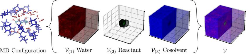
http://zavalab.engr.wisc.edu

optimal operators (and associated features) that best map the input data to the output data. For in-
stance, in recognizing an image (the input), the CNN seeks to learn the patterns of the image that
best explains a label given to an image (the output).
    The earliest version of a CNN was proposed in 1980 by Kunihiko Fukushima [8] and was used
for pattern recognition. In the late 1980s, the LeNet model proposed by LeCun et al. introduced
the concept of backward propagation, which streamlined learning computations using optimization
techniques [19]. Although the LeNet model had a simple architecture, it was capable of recognizing
hand-written digits with high accuracy. In 1998, Rowley et al. proposed a CNN model capable of
performing face recognition tasks (this work revolutionized object classification and detection) [29].
The complexity of CNN models (and their predictive power) has dramatically expanded with the
advent of parallel computing architectures such as graphics processing units [25]. Modern CNN
models for image recognition include SuperVision [18], GoogLeNet [35], VGG [32], and ResNet [10].
New models are currently being developed to perform diverse computer vision tasks such as object
detection [27], semantic segmentation [20], action recognition [31], and 3D analysis [15]. Nowadays,
CNNs are routinely used in applications such as in the face-unlock feature of smartphones [24].
    CNNs tend to outperform other machine learning models (e.g., support vector machine and de-
cision tree) but their behavior is difficult to explain. For instance, it is not always straightforward to
determine the features that the operators are seeking to extract. As such, researchers have devoted
significant effort into understanding the mathematical properties of CNNs. For instance, Cohen et
al. established an equivalence between CNNs and hierarchical tensor factorizations [5]. Bruna et al.
analyzed feature extraction capabilities [2] and showed that these satisfy translation invariance and
deformation stability (important concepts in determining geometric features from data).
    While CNNs were originally developed to perform computer vision tasks, the grid data repre-
sentation used by CNNs is flexible and can be used to process datasets arising in many different
applications. For instance, in the field of chemistry, Hirohara et al. proposed a matrix representa-
tions of SMILES strings (which encodes molecular topology) by using a technique known as one-hot
encoding [13]. The authors used this representation to train a CNN that could predict the toxicity
of chemicals; it was shown that the CNN outperformed traditional models based on fingerprints (an
alternative molecular representation). Via analysis of the learned filters, the authors also determined
chemical structures (features) that drive toxicity. In the realm of biology, Xie et al. applied CNNs
to count and detect cells from micrographs [39]. In area of material science, Smith et al. have used
CNNs to extract features from optical micrographs of liquid crystals to design chemical sensors [33].
    While there has been extensive research on CNNs and the number of applications in science and
engineering is rapidly growing, there are limited reports available in the literature that outline the
mathematical foundations and operations behind CNNs. As such, important connections between
CNNs and other fields such as statistics, signal processing, linear algebra, differential equations,
and optimization remain under-appreciated. We believe that this disconnect limits the ability of
researchers to propose extensions and identify new applications. For example, a common miscon-
ception is that CNNs are only applicable to computer vision tasks; however, CNNs can operate on
general grid data objects (vectors, matrices, and tensors). Moreover, operators learned by CNNs
can be potentially explained when analyzed from the perspective of calculus and statistics. For in-

                                                    2
http://zavalab.engr.wisc.edu

stance, certain types of operators seek to extract gradients (derivatives) of a field or seek to extract
correlation structures. Establishing connections with other mathematical fields is important in gain-
ing interpretability of CNN models. Understanding the operations that take place in a CNN is also
important in order to understand their inherent limitations, in proposing potential modeling and al-
gorithmic extensions, and in facilitating the incorporation of CNNs in computational workflows of
interest to engineers (e.g., process monitoring, control, and optimization).

    In this work, we review the mathematical foundations of CNNs; specifically, we provide concise
derivations of input data representations and of convolution operations. We explain the origins of
certain types of operators and the data transformations that they induce to highlight features that are
hidden in the data. Moreover, we provide concise derivations for forward and backward propaga-
tions that arise in CNN training procedures. These derivations provide insight into how information
flows in the CNN and help understand computations involved in the learning process (which seeks
to solve an optimization problem that minimizes a loss function). We also explain how derivatives
of the loss function can be used to understand key features that the CNN searches for to make pre-
dictions. We illustrate the concepts by applying CNNs to new types of applications such as optimal
control (1D) , flow cytometry (2D), multivariate process monitoring (2D), and molecular simulations
(3D). Specifically, we focus our attention on how to convert raw data into a suitable grid-like repre-
sentation that the CNN can process.

2 Convolution Operations

Convolution is a mathematical operation that involves an input function and an operator function
(these functions are also known as signals). A related operation that is often used in CNNs is cross-
correlation. Although technically different, the essence of these operations is similar (we will see that
they are mirror representations). One can think of a convolution as an operation that seeks to trans-
form the input function in order to highlight (or extract) features. The input and operator functions
can live on arbitrary dimensions (1D, 2D, 3D, and higher). The features highlighted by an operator
are defined by its design; for instance, we will see that one can design operators that extract spe-
cific patterns, derivatives (gradients), or frequencies. These features encode different aspects of the
data (e.g., correlations and geometrical patterns) and are often hidden. Input and operator functions
can be continuous or discrete; discrete functions facilitate computational implementation but contin-
uous functions can help understand and derive mathematical properties. For example, families of
discrete operators can be generated by using a single continuous function (a kernel function). We
begin our discussion with 1D convolution operations and we later extend the analysis to the 2D case;
extensions to higher dimensions are straightforward once the basic concepts are outlined. We high-
light, however, that convolutions in high dimensions are computationally expensive (and sometimes
intractable).

                                                   3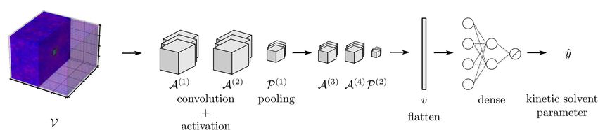
http://zavalab.engr.wisc.edu

2.1 1D Convolution Operations

The convolution of scalar continuous functions u : R 7→ R and v : R 7→ R is denoted as ψ = u ∗ v and
their cross-correlation is denoted as φ = u ⋆ v. These operations are given by:
                                          Z ∞
                                               u x′ · v x − x′ dx′ , x ∈ (−∞, ∞)

                     ψ (x) = (u ∗ v)(x) =                                                        (1a)
                                           −∞
                                          Z ∞
                                               u x′ · v x + x′ dx′ , x ∈ (−∞, ∞).

                     φ (x) = (u ⋆ v)(x) =                                                        (1b)
                                          −∞

We will refer to function u as the convolution operator and to v as the input signal. The output of
the convolution operation is a scalar continuous function ψ : R 7→ R that we refer to as the convolved
signal. The output of the cross-correlation operation is also a continuous function φ : R 7→ R that we
refer to as the cross-correlated signal.

    The convolution and cross-correlation are applied to the signal by spanning the domain x ∈
(−∞, ∞); we can see that convolution is applied by looking backward, while cross-correlation is ap-
plied by looking forward. One can show that cross-correlation is equivalent to convolution that uses
a rotated (flipped) operator u by 180 degrees; in other words, if we define the rotated operator as −u
then u ∗ v = (−u) ⋆ v. We thus have that convolution and cross-correlation are mirror operations;
consequently, convolution and cross-correlation are often both referred to as convolution. In what fol-
lows we use the term convolution and cross-correlation interchangeably; we highlight one operation
over the other when appropriate. Modern CNN packages such as PyTorch [26] use cross-correlation
in their implementation (this is more intuitive and easier to implement).

Figure 1: From top to bottom: Input signal v, Gaussian and triangular operators u, convolved signal
ψ, and cross-correlated signal φ.

   One can think of convolution and cross-correlation as weighting operations (with weighting func-

                                                  4
http://zavalab.engr.wisc.edu

tion defined by the operator). The weighting function u can be designed in different ways to perform
different operations to the signal v such as averaging, smoothing, differentiation, and pattern recog-
nition. In Figure 1 we illustrate the application of a Gaussian operator u to a noisy rectangular signal
v. We note that the convolved and cross-correlated signals are identical (because the operator is sym-
metric and thus u = −u). We also note that the output signals are smooth versions of the input signal;
this is because a Gaussian operator has the effect of extracting frequencies from the signal (a fact that
can be established from Fourier analysis). Specifically, we recall that the Fourier transform of the
convolved signal ψ satisfies:
                                    F{ψ} = F{u ∗ v} = F{u} · F{v}.                                    (2)

where F{w} is the Fourier transform of scalar function w. Here, the product F{u} · F{v} has the
effect of preserving the frequencies in the signal v that are also present in the operator u. In other
words, convolution acts as a filter of frequencies; as such, one often refers to operators as filters. By
comparing the output signals of convolution and cross-correlation obtained with the triangular op-
erator, we can confirm that one is the mirror version of the other. From Figure 1, we also see that
the output signals are smooth variants of the input signal; this is because the triangular operator also
extracts frequencies from the input signal (but the extraction is not as clean as that obtained with the
Gaussian operator). This highlights the fact that different operators have different frequency content
(known as the frequency spectrum).

    Convolution and cross-correlation are implemented computationally by using discrete represen-
tations; these signals are represented by column vectors u ∈ Rn and v ∈ Rn with entries denoted as
u[x], v[x], x = −N, ..., N (note that n = 2 · N + 1). Here, we note that the input and operator are
defined over a 1D grid. The discrete convolution results in vector ψ ∈ Rn with entries given by:
                                       N
                                       X
                                                u x′ · v x + x′ , x ∈ {−N, N }.

                            ψ [x] =                                                                   (3)
                                      x′ =−N

Here, we use {−N, N } to denote the integer sequence −N, −N + 1, ..., −1, 0, 1, ..., N − 1, N . We
note that computing ψ [x] at a given location x requires n operations and thus computing the entire
output signal (spanning x ∈ {−N, N }) requires n2 operations; consequently, convolution becomes
expensive when the signal and operator are long vectors; as such, the operator u is often a vector
of low dimension (compared to the dimension of the signal v). Specifically, consider the operator
u ∈ Rnu with entries u[x], x = −Nu , ..., Nu (thus nu = 2 · Nu + 1) and assume nu ≪ n (typically
nu = 3). The convolution is given by:
                                       Nu
                                       X
                                                u x′ · v x + x′ , x ∈ {−N, N }.

                           ψ [x] =                                                                    (4)
                                      x′ =−Nu

This reduces the number of operations needed from n2 to n · nu .

   The convolved signal is obtained by using a moving window starting at the boundary x = −N and
by moving forward as x+1 until reaching x = N . We note that the convolution is not properly defined

                                                        5
http://zavalab.engr.wisc.edu
close to the boundaries (because the window lies outside the domain of the signal). This situation can
be remedied by starting the convolution at an inner entry of v such that the full window is within the
signal (this gives a proper convolution). However, this approach has the effect of returning a signal
ψ that is smaller than the original signal v. This issue can be overcome by artificially padding the
signal by adding zero entries (i.e., adding ghost entries to the signal at the boundaries). This is an
improper convolution but returns a signal ψ that has the same dimension as v (this is often convenient
for analysis and computation). Figure 2 illustrates the difference between convolutions with and
without padding. We also highlight that it is possible to advance the moving window by multiple
entries as x + s (here, s ∈ Z+ is known as the stride). This has the effect of reducing the number
of operations (by skipping some entries in the signal) but returns a signal that is smaller than the
original one.
Figure 2: Illustration of 1D convolution with (bottom) and without (top) zero-padding.
By defining signals u ∈ Rnu and v ∈ Rnv with entries u[x], x = 1, ..., nu and v[x], x = 1, ..., nv , one
can also express the valid convolution operation in an asymmetric form as:
m
X
u x′ · v x + x′ − 1 , x ∈ {1, nv − nu + 1}.
ψ [x] = (5)
x′ =1
In CNNs, one often applies multiple operators to a single input signal or one analyzes input sig-
nals that have multiple channels. This gives rise to the concepts of single-input single-output (SISO),
single-input multi-output (SIMO), and multi-input multi-output (MIMO) convolutions.
In SISO convolution, we take a 1-channel input vector and output a vector (a 1-channel signal), as
in (5). In SIMO convolution, one uses a single input v ∈ Rnv and a collection of q operators U(j) ∈ Rnu
with j ∈ {1, q}. Here, every element U(j) is an nu -dimensional vector and we represent the collection
as the object U . SIMO convolution yields a collection of convolved signals Ψ(j) ∈ Rnv −nu +1 with
j ∈ {1, q} and with entries given by:
m
X
U(j) x′ · v x + x′ − 1 , x ∈ {1, nv − nu + 1}.
Ψ(j) [x] = (6)
x′ =1
In MIMO convolution, we consider a multi-channel input given by the collection V(i) ∈ Rnv , i ∈
{1, p} (p is the number of channels); the collection is represented as the object V. We also consider a
6http://zavalab.engr.wisc.edu
collection of operators U(i,j) ∈ Rnu with i ∈ {1, p} and j ∈ {1, q}; in other words, we have q operators
per input channel i ∈ {1, p} and we represent the collection as the object U . MIMO convolution yields
the collection of convolved signals Ψ(j) ∈ Rnv −nu +1 with j ∈ {1, q} and with entries given by:
p
X
Ψ(j) [x] = U(i,j) ∗ V(i)
i=1
p X m
(7)
X
U(i,j) x′ · V(i) x + x′ − 1 , x ∈ {1, nv − nu + 1}.
=
i=1 x′ =1
We see that, in MIMO convolution, we add the contribution of all channels i ∈ {1, p} to obtain the
output object Ψ, which contains j ∈ {1, q} channels given by vectors Ψ(i) of dimension (nv − nu + 1).
Channel combination loses information but saves computer memory.
2.2 2D Convolution Operations
Convolution and cross-correlation operations in 2D are analogous to those in 1D; the convolution and
cross-correlation of a continuous operator u : R2 7→ R and an input signal v : R2 7→ R are denoted as
ψ = u ∗ v and φ = u ⋆ v and are given by:
Z ∞Z ∞
u x′1 , x′2 · v x1 − x′1 , x2 − x′2 dx′1 dx′2 ,
ψ (x1 , x2 ) = x1 , x2 ∈ (−∞, ∞) (8a)
−∞ −∞
Z ∞Z ∞
u x′1 , x′2 · v x1 + x′1 , x2 + x′2 dx′1 dx′2 ,
φ (x1 , x2 ) = x1 , x2 ∈ (−∞, ∞) (8b)
−∞ −∞
As in the 1D case, the terms convolution and cross-correlation are used interchangeably; here, we
will use the cross-correlation form (typically used in CNNs).
In the discrete case, the input signal and the convolution operator are matrices U ∈ RnU ×nU and
V ∈ RnV ×nV with entries U [x1 , x2 ] , x1 , x2 ∈ {−NU , NU } and V [x1 , x2 ] , x1 , x2 ∈ {−NV , NV } (thus
nU = 2 · NU + 1 and nV = 2 · NV + 1). For simplicity, we assume that these are square matrices and
we note that the input and operator are defined over a 2D grid. The convolution of the input and
operator matrices results in a matrix Ψ = U ∗ V with entries:
NU
X NU
X
U x′1 , x′2 · V x1 + x′1 , x2 + x′2 , x1 , x2 ∈ {−NV , NV }.
Ψ [x1 , x2 ] = (9)
x′1 =−NU x′2 =−NU
In Figure 3 we illustrate 2D convolutions with and without padding. The 2D convolution (in valid
and asymmetric form) can be expressed as:
nU X
X nU
U x′1 , x′2 · V x1 + x′1 − 1, x2 + x′2 − 1 ,
Ψ [x1 , x2 ] = (10)
x′1 =1 x′2 =1
where x1 ∈ {1, nV − nU + 1}, x2 ∈ {1, nV − nU + 1} and Ψ ∈ R(nV −nU +1)×(nV −nU +1) .
The SISO convolution of an input V ∈ RnV ×nV and an operator U ∈ RnU ×nU is given by (10)
and outputs a matrix Ψ ∈ R(nV −nU +1)×(nV −nU +1) . In SIMO convolution, we are given a collection
7http://zavalab.engr.wisc.edu
Figure 3: Illustration of 2D convolution with (bottom) and without (top) zero padding.
of operators U(j) ∈ RnU ×nU with j ∈ {1, q}. A convolved matrix Ψ(j) ∈ R(nV −nU +1)×(nV −nU +1) is
obtained by applying the j-th operator U(j) to the input V :
nU X
X nU
U(j) x′1 , x′2 V x1 + x′1 − 1, x2 + x′2 − 1
Ψ(j) [x1 , x2 ] = (11)
x′1 =1 x′2 =1
for j ∈ {1, q}, x1 , x2 ∈ {1, nV −nU +1}. The collection of convolved matrices Ψ(j) ∈ R(nV −nU +1)×(nV −nU +1) , j ∈
{1, q} is represented as object Ψ.
In MIMO convolution, we are given a p-channel input collection V(i) ∈ RnV ×nV with i ∈ {1, p}
and represented as V. We convolve this input with the operator object U , which is a collection
U(i,j) ∈ RnU ×nU , i ∈ {1, p}, j ∈ {1, q}. This results in an object Ψ given by the collection Ψ(j) ∈
R(nV −nU +1)×(nV −nU +1) for j ∈ {1, q} and with entries given by:
p
X
Ψ(j) [x1 , x2 ] = U(i,j) ∗ V(i)
i=1
p X nU X nU (12)
X
U(i,j) x′1 , x′2 x′1 x′2
= V(i) x1 + − 1, x2 + −1 ,
i=1 x′1 =1 x′2 =1
for j ∈ {1, q}, x1 ∈ {1, nV −nU +1}, and x2 ∈ {1, nV −nU +1}. For convenience, the input object is often
represented as a 3D tensor V ∈ RnV ×nV ×p , the convolution operator is represented as the 4D tensor
U ∈ RnU ×nU ×p×q , and the output signal is represented as the 3D tensor Ψ ∈ R(nV −nU +1)×(nV −nU +1)×q .
We note that, if p = 1 and q = 1 (1-channel inputs and channels), these tensors become matrices.
Tensors are high-dimensional quantities that require significant computer memory to store and sig-
nificant power to process.
8http://zavalab.engr.wisc.edu
Figure 4: MIMO convolution of an RGB image V ∈ R50×50×3 (3-channel input) corresponding to a
liquid crystal micrograph. The red, green, and blue (RGB) channels of the input 3D tensor V are
convolved with an operator U ∈ R3×3×3×1 (a 3D tensor since q = 1) that contains a Sobel operator
(for edge detection), Gaussian operator (for blurring), and Laplacian operator (for edge detection).
The output Ψ ∈ R48×48×1 is a matrix (since q = 1) that results from the combination of the convolved
matrices.
MIMO convolutions in 2D are typically used to process RGB images (3-channel input), as shown
in Figure 4. Here, the RGB image is the object V and each input channel V(i) is a matrix; each of these
matrices is convolved with an operator U(i,1) . Here we assume q = 1 (one operator per channel). The
collection of convolved matrices Ψ(i,1) are combined to obtain a single matrix Ψ(1) . If we consider a
collection of operators U(i,j) with i ∈ {1, p}, j ∈ {1, q} and q > 1, the output of MIMO convolution re-
turns the collection of matrices Ψ(j) with j ∈ {1, q}, which is assembled in the tensor Ψ. Convolution
with multiple operators allows for the extraction of different types of features from different channels.
We highlight that the use of channels is not restricted to images; specifically, channels can be used
to input data of different variables in a grid (e.g., temperature, concentration, density). As such,
channels provide a flexible framework to express multivariate data.
We also highlight that a grayscale image is a 1-channel input matrix (the RGB channels are com-
bined in a single channel). In a grayscale image, every pixel (an entry in the associated matrix) has
a certain light intensity value; whiter pixels have higher intensity and darker pixels have a lower in-
tensity (or the other way around). The resolution of the image is dictated by the number of pixels and
thus dictates the size of the matrix; the size of the matrix dictates the amount of memory needed for
storage and computations needed for convolution. It is also important to emphasize that any matrix
9http://zavalab.engr.wisc.edu
can be visualized as a grayscale image (and any grayscale image has an underlying matrix). This duality
is important because visualizing large matrices (e.g., to identify patterns) is difficult if one directly
inspects the numerical values; as such, a convenient approach to analyze patterns in large matrices
consists of visualizing them as images.
Finally, we highlight that convolution operators can be applied to any grid data object in higher
dimensions (e.g., 3D and 4D) in a similar manner. Convolutions in 3D can be used to process video
data (each time frame is an image). However, 3D data objects can also be used to represent data
distributed over 3D Euclidean spaces (e.g., density or flow in a 3D domain). However, the complexity
of convolution operations in 3D (and higher dimensions) is substantial. In the discussion that follows
we focus our attention to 2D convolutions; in Section 6 we illustrate the use of 3D convolutions in a
practical application.
3 Convolution Operators
Convolution operators are the key functional units that a CNN uses to extract features from input
data objects. Some commonly used operators and their transformation effect are shown in Figure
4. When the input is convolved with a Sobel operator, the output highlights the edges (gradients
of intensity). The reason for this is that the Sobel operator is a differential operator. To explain this
concept, consider a discrete 1D signal v; its derivative at entry x can be computed using the finite
difference:
v[x + 1] − v[x − 1]
v ′ [x] = . (13)
2
This indicates that we can compute the derivative signal v ′ by applying a convolution of the form
v ′ = u ∗ v with operator u = (1/2, 0, −1/2). Here, the operator can be scaled as u = (1, 0, −1) as this
does not alter the nature of the operation performed (just changes the scale of the entries of v ′ ).
The Sobel operator shown in Figure 4 is a 3 × 3 matrix of the form:
1 2 1 1 h i
U = 0 0 0 = 0 1 2 1 , (14)
−1 −2 −1 −1
where the vector (1, 0, −1) approximates the first derivative in the vertical direction, and (1, 2, 1) is a
binomial operator that smooths the input matrix.
Another operator commonly used to detect edges in images is the Laplacian operator; this oper-
∂2 ∂2
ator is an approximation of the continuous Laplacian operator L = ∂x 2 + ∂x2 . The convolution of a
1 2
matrix V using a 3 × 3 Laplacian operator U is:
U ∗ V = V [x1 − 1, x2 ] + V [x1 + 1, x2 ] + V [x1 , x2 − 1] + V [x1 , x2 + 1] − 4 · V [x1 , x2 ] . (15)
10http://zavalab.engr.wisc.edu
This reveals that the convolution is an approximation of L that uses a 2D finite difference scheme;
this scheme has an operator of the form:
0 1 0
U = 1 −4 1 . (16)
0 1 0
The transformation effect of the Laplacian operator is shown in Figure 4. In the partial differential
equations (PDE) literature, the non-zero structure of a finite-difference operator is known as the sten-
cil. As expected, a wide range of finite difference approximations (and corresponding operators) can
be envisioned. Importantly, since the Laplacian operator computes the second derivative of the input,
this is suitable to detect locations of minimum or maximum intensity in an image (e.g., peaks). This
allows us to understand the geometry of matrices (e.g., geometry of images or 2D fields). Moreover,
this also reveals connections between PDEs and convolution operations.
The Gaussian operator is commonly used to smooth out images. A Gaussian operator is defined
by the density function:
1 − x21 +x2 22
U (x1 , x2 ) = e 2σ , (17)
2πσ 2
where σ ∈ R+ is the standard deviation. The standard deviation determines the spread of of the
operator and is used to control the frequencies removed from a signal. We recall that the density
of a Gaussian is maximum at the center point and decays exponentially (and symmetrically) when
moving away from the center. Discrete representations of the Gaussian operator are obtained by
manipulating σ and truncating the density in a window. For instance, the 3 × 3 Gaussian operator as
shown in Figure 4 is:
1 2 1
1
U= 2 4 2 . (18)
16
1 2 1
Here, we can see that the operator is square and symmetric, has a maximum value at the center point,
and the values decay rapidly as one moves away from the center.
Convolution operators can also be designed to perform pattern recognition; for instance, consider
the situation in which you want to highlight areas in a matrix that have a pattern (feature) of interest.
Here, the structure of the operator dictates the 0-1 pattern sought. For instance, in Figure 5 we present
an input matrix with 0-1 entries and we perform a convolution with an operator with a pre-defined
0-1 structure. The convolution highlights the areas in the input matrix in which the presence of the
sought pattern is strongest (or weakest). As one can imagine, a huge number of operators could be
designed to extract different patterns (including smoothing and differentiation operators); moreover,
in many cases it is not obvious which patterns or features might be present in the image. This indi-
cates that one requires a systematic approach to automatically determine which features of an input
signal (and associated operators) are most relevant.
11http://zavalab.engr.wisc.edu
Figure 5: Highlighting sought patterns by convolutional operators. When the sought pattern is
matched, the convolution generates a large signal.
4 CNN Architectures
CNNs are hierarchical (layered) models that perform a sequence of convolution, activation, pool-
ing, flattening operations to extract features from input data object. The output of this sequence
of transformation operations is a vector that summarizes the feature information of the input; this
feature vector is fed to a fully-connected neural net that makes final predictions. The goal of the
CNN is to determine the features of a set of input data objects (input data samples) that best predict
the corresponding output samples. Specifically, the input of the CNN are a set of sample objects
V (i) ∈ RnV ×nV ×p with sample index i ∈ {1, n}, and the output of the CNN are the corresponding
predicted labels ŷ[i], i ∈ {1, n}. The goal of a CNN is to determine convolution operators giving
features that best match the predicted labels to the output labels; in other words, the CNN seeks to
find operators (and associated features) that best map the inputs to the outputs.
In this section we discuss the different elements of a 2D CNN architecture. To facilitate the anal-
ysis, we construct a simple CNN of the form shown in Figure 6. This architecture contains a single
layer that performs convolution, activation, pooling, and flattening. Generalizing the discussion to
multiple layers and higher dimensions (e.g., 3D) is rather straightforward once the basic concepts
are established. Also, in the discussion that follows, we consider a single input data sample (that we
denote as V) and discuss the different transformation operations performed to it along the CNN to
obtain a final prediction (that we denote as ŷ). We then discuss how to combine multiple samples to
train the CNN.
4.1 Convolution Block
An input sample of the CNN is the tensor V ∈ RnV ×nV ×p . The convolution block uses the operator
U ∈ RnU ×nU ×p×q to conduct a MIMO convolution. The output of this convolution is the tensor
Ψ ∈ RnΨ ×nΨ ×q with entries given by:
p X
X nU X
nU
U(i,j) x′1 , x′2 V(i) x1 + x′1 − 1, x2 + x′2 − 1 ,
Ψ(j) [x1 , x2 ] = bc [j] + (19)
i=1 x′1 =1 x′2 =1
12http://zavalab.engr.wisc.edu
Figure 6: CNN architecture (top) comprised of a convolution block fc , a max-pooling block fp , a
flattening block ff , and a dense block fd . Here, hc and hd are activations applied in the convolution
and dense blocks, respectively. A sample input is a p-channel object V ∈ RnV ×nV ×p and the predicted
output is a scalar ŷ ∈ R. The parameters of the CNN are U , bc (for convolution block) and w, bd
(for dense block). During training (bottom), forward propagation processes the sample input and
outputs a scalar, and backward propagation calculates the gradients by recursively using chain-rules
from the output to the input.
where x1 ∈ {1, nΨ }, x2 ∈ {1, nΨ }, and j ∈ {1, q}. A bias parameter bc [j] ∈ R is added after the con-
volution operation; the bias helps adjust the magnitude of the convolved signal. To enable compact
notation, we define the convolution block using the mapping Ψ = fc (V; U , bc ); here, we note that the
mapping depends on the parameters U (the operators) and bc (the bias). An example of a convolution
block with a 3-channel input and 2-channel operator is shown in Figure 7.
Figure 7: Convolution block for a 3-channel input V ∈ R4×4×3 and a 2-channel operator U ∈
R3×3×3×2 . The output Ψ ∈ R2×2×2 is obtained by combining the contributions of the different chan-
nels. A bias bc is added to this combination to give the final output of the convolution block.
13http://zavalab.engr.wisc.edu
4.2 Activation Block
The convolution block outputs the signal Ψ; this is passed through an activation block given by
the mapping A = hc (Ψ) with A ∈ RnΨ ×nΨ ×q . Here, we define an activation mapping of the form
hc : RnΨ ×nΨ ×q 7→ RnΨ ×nΨ ×q . The activation of Ψ is conducted element-wise as:
A(i) [x1 , x2 ] = α Ψ(i) [x1 , x2 ] , (20)
where α : R 7→ R is an activation function (a scalar function). Typical activation functions include the
sigmoid, hyperbolic tangent (tanh), and Rectified Linear Unit (ReLU):
1
αsig (z) =
1 + e−z
αtanh (z) = tanh (z) (21)
αReLU (z) = max (0, z) ,
Figures 8 and 9 illustrate the transformation induced by the activation functions. These functions
act as basis functions that, when combined in the CNN, enable capturing nonlinear behavior. A com-
mon problem with sigmoid and tanh functions is that they exhibit the so-called vanishing gradient
effect [9]. Specifically, when the input values are large or small in magnitude, the gradient of the sig-
moid and tanh functions is small (flat at both ends) and this makes the activation output insensitive
to changes in the input. Furthermore, both the sigmoid and tanh functions are sensitive to the change
in input when the output is close to 1/2 and zero, respectively. The ReLU function is commonly used
to avoid vanishing gradient effects and to increase sensitivity [23]. This activation function outputs a
value of zero when the input is less than or equal to zero, but outputs the input value itself when the
input is greater than zero. The function is linear when the input is greater than zero, which makes
the CNN easier to optimize with gradient-based methods [9]. However, ReLU is not continuously
differentiable when the input is zero; in practice, CNN implementations assume that the gradient is
zero when the input is zero.
Figure 8: Output of the sigmoid, tanh and ReLU functions on a fixed domain.
14http://zavalab.engr.wisc.edu
Figure 9: Element-wise activation of matrix Ψ (a convolved micrograph) in the convolutional block.
4.3 Pooling Block
The pooling block is a transformation that reduces the size of the output obtained by convolution and
subsequent activation. This block also seeks to make the representation approximately invariant to
small translation of the inputs [9]. Max-pooling and average-pooling are the most common pooling
operations (here we focus on max-pooling). The pooling operation P = fp (A) can be expressed
as a mapping fp : RnΨ ×nΨ ×q 7→ R⌊nΨ /np ⌋×⌊nΨ /np ⌋×q and delivers a tensor P ∈ R⌊nΨ /np ⌋×⌊nΨ /np ⌋×q .
To simplify the discussion, we denote nP = ⌊nΨ /np ⌋; the max-pooling operation with i ∈ {1, q} is
defined as:
P(i) [x1 , x2 ] = max{A(i) (x1 − 1) nU + n′U , (x2 − 1) nU + n′U , n′U ∈ {1, nU }, n′U ∈ {1, nU }},
(22)
where x1 ∈ {1, nP }, x2 ∈ {1, nP }. In Figure 10, we illustrate the max-pooling and averaging pooling
operations on a 1-channel input.
Figure 10: Max-pooling and average-pooling operations with a 2×2 pooling window size. Each entry
in the output feature map P ∈ R2×2 is the maximum (or average) value of the corresponding pooling
window in the input A ∈ R2×2 .
Operations of convolution, activation, and pooling constitute a convolution unit and deliver an
output object P = fp (hc (fc (V)). This object can be fed into another convolution unit to obtain a
new output object P = fp (hc (fc (P)) and this recursion can be performed over multiple units. The
15http://zavalab.engr.wisc.edu
recursion has the effect of highlighting different features of the input data object V (e.g., that capture
local and global patterns). In our discussion we consider a single convolution unit.
4.4 Flattening Block
The convolution, activation, and pooling blocks deliver a tensor P ∈ RnP ×nP ×p that is flattened to
a vector v ∈ RnP ·nP ·p ; this vector is fed into a fully-connected (dense) block that performs the final
prediction. The vector v is typically known as the feature vector. The flattening block is represented as
the mapping ff : RnP ×nP ×p 7→ Rnv with nv = nP · nP · p that outputs v = ff (P). Note that this block
is simply a vectorization of a tensor.
Figure 11: After flattening P to a vector v, the flatting block maps v to d. The lines between v and d
represent the dense connectivity induced by the weight vector w. A bias bd is added after weighting.
The prediction ŷ is obtained by activating d.
4.5 Prediction (Dense) Block
The feature vector v ∈ Rnv is input into a prediction block that delivers the final prediction ŷ ∈ R.
This block is typically a fully-connected (dense) neural net with multiple weighting and activation
units (here we only consider a single unit). The prediction block first mixes the elements of the feature
vector as:
d = w T v + bd , (23)
where w ∈ Rnv is the weighting (parameter) vector and bd ∈ R is the bias parameter. The vector
d ∈ R is normally known as the evidence. We denote the weighting operation using the mapping fd :
Rnv 7→ R and thus d = fd (v; w, bd ). In Figure 11, we illustrate this weighting operation. An activation
function is applied to the evidence d to obtain the final prediction ŷ = hd (d) with hd : R 7→ R. This
involves an activation (e.g., with a sigmoidal or ReLU function). We thus have that the prediction
block has the form ŷ = hd (fd (v)). One can build a multi-layer fully-connected network by using a
recursion of weighting and activation steps (here we consider one layer to simplify the exposition).
Here, we assume that the CNN delivers a single (scalar) output ŷ. In practice, however, a CNN can
also predict multiple outputs; in such a case, the weight parameter becomes a matrix and the bias is a
vector. We also highlight that the predicted output can be an integer value (to perform classification
tasks) or a continuous value (to perform regression tasks).
16http://zavalab.engr.wisc.edu
5 CNN Training
CNN training aims to determine the parameters (operators and biases) that best map the input data
to the output data. The fundamental operations in CNN training are forward and backward propaga-
tion, which are used by an optimization algorithm to improve parameters. In forward propagation,
the input data is propagated forward through the CNN (block by block and layer by layer) to make
a prediction and evaluate a loss function that captures the mismatch between the predicted and true
output. In backward propagation, one computes the gradient of the loss function with respect to
each parameter via a recursive application of the chain rule of differentiation (block by block layer
by layer). This recursion starts in the prediction block and proceeds backwards to the convolution
block. Notably, we will see that the derivatives of the transformation blocks have explicit (analytical)
representations.
5.1 Forward Propagation
To explain the process of forward propagation, we consider the CNN architecture shown in Figure 6
with an input V ∈ RnV ×nV ×p and an output (prediction) ŷ ∈ R. All parameters U ∈ RnU ×nU ×p×q ,
bc ∈ Rq , w ∈ Rnv and bd ∈ R are flattened and concatenated to form a parameter vector θ ∈ Rnθ ,
where nθ = nU · nU · p · q + q + nV + 1. We can express the entire sequence of operations carried out in
the CNN as a composite mapping F : RnV ×nV ×p 7→ R and thus ŷ = F (V; θ). We call this mapping the
forward propagation mapping (shown in Figure 6) and note that this can be decomposed sequentially
(via lifting) as:
ŷ = F (V; θ)
= F (V; U , bc , w, bd ) (24)
= hd (fd (ff (fp (hc (fc (V; U , bc )))) ; w, bd )) .
This reveals the nested nature and the order of the CNN transformations on the input data. Specifi-
cally, we see that one conducts convolution, activation, pooling, flattening, and prediction.
To perform training, we collect a set of input samples V (i) ∈ RnV ×nV ×p and corresponding output
labels y[i] ∈ R with sample index i ∈ {1, n}. Our aim is to compare the true output labels y[i] to
the CNN predictions ŷ[i] = F V (i) ; θ . To do so, we define the loss function L : Rn → R that we
aim to minimize. For classification tasks, the output ŷ[i] is binary and a common loss function is the
cross-entropy [14]:
n
1X
L (ŷ) = − [y[i] log (ŷ[i]) + (1 − y[i]) log (1 − ŷ[i])] , (25)
n
i=1
For regression tasks, we have that the output ŷ (i) is continuous and a common loss function is the
mean squared error:
n
1X
L (ŷ) = (y[i] − ŷ[i])2 . (26)
n
i=1
17http://zavalab.engr.wisc.edu
In compact form, we can write the loss function as L (F (V; θ)) = L (θ). Here, V contains all the input
samples V (i) for i ∈ {1, n}. The loss function can be decomposed into individual samples and thus
we can express it as:
n
1 X (i)
L (ŷ) = L (θ). (27)
n
i=1
where L(i) (θ) is the contribution associated with the i-th data sample.
5.2 Optimization Algorithms
The parameters of the CNN are obtained by finding a solution to the optimization problem:
min L(θ). (28)
θ
The loss function L embeds the forward propagation mapping F (which is a highly nonlinear map-
ping); as such, the loss function might contain many local minima (and such minima tend to be flat).
We recall that appearance of flat minima is often the manifestation of model overparameterization;
this is due to the fact that the parameter vector θ can contain hundreds of thousands to millions of
values. As such, training of CNNs need to be equipped with appropriate validation procedures (to
ensure that the model generalizes well). Most optimization algorithms used for CNNs are gradient-
based (first-order); this is because second-order optimization methods (e.g., Newton-based) involve
calculating the Hessian of the loss function L with respect to parameter vector θ, which is compu-
tationally expensive (or intractable). Quasi-Newton methods (e.g., limited-memory BFGS) are also
often used to train CNNs.
Gradient descent (GD) is the most commonly used algorithm to train CNNs. This algorithm
updates the parameters as:
θ ← θ − η · ∆θ (29)
where η ∈ R+ is the learning rate (step length) and ∆θ ∈ Rnθ is the step direction. In GD, the
step direction is set to ∆θ = ∇θ L(θ) (the gradient of the loss). Since the loss function is a sum over
samples, the gradient can be decomposed as:
n
1X
∇θ L (θ) = ∇θ L(i) (θ). (30)
n
i=1
Although GD is easy to compute and implement, θ is not updated until the gradient of the entire
dataset is calculated (which can contain millions of data samples). In other words, the parameters are
not updated until all the gradient components ∇θ L(i) (θ) are available. This leads to load-imbalancing
issues and limits the parallel scalability of the algorithm.
Stochastic gradient descent (SGD) is a variant of GD that updates θ more frequently (with gra-
dients from a partial number of samples). Specifically, θ changes after calculating the loss for each
sample. SGD updates the parameters by using the step ∆θ = ∇θ L(i) (θ), where sample i is selected at
18http://zavalab.engr.wisc.edu
random. Since θ is updated frequently, SGD requires less memory and has better parallel scalability
[17]. Moreover, it has been shown empirically that this algorithm has the tendency to escape local
minima (it explores the parameter space better). However, if the training sample has high variance,
SGD will converge slowly.
Mini-batch GD is an enhancement of SGD; here, the entire dataset is divided into b batches and θ
is updated after calculating the gradient of each batch. This results in a step direction of the form:
1 X
∆θ = ∇θ L(j) (θ) . (31)
b (i)
j∈B
where B (i) is a set of sample corresponding to batch i ∈ {1, b} and the entries of the batches are
selected at random. Mini-batch GD updates the model parameters frequently and has faster conver-
gence in the presence of high variance [37].
5.3 Backward Propagation
Backward propagation (backpropagation) seeks to compute elements of the gradient of the loss
∇θ L(i) (θ) by recursive use of the chain rule. This approach exploits the nested nature of the forward
propagation mapping:
ŷ = hd (fd (ff (fp (hc (fc (V; U , bc )))) ; w, bd )) . (32)
This mapping can be expressed in backward form as:
ŷ = hd (d) (33a)
d = fd (v; w, bd ) (33b)
v = ff (P) (33c)
P = fp (A) (33d)
A = hc (Ψ) (33e)
Ψ = fc (V; U , bc ) (33f)
An illustration of this backward sequence is presented in Figure 6. Exploiting this structure is essen-
tial to enable scalability (particularly for saving memory). To facilitate the explanation, we consider
the squared error loss defined for a single sample (generalization to multiple samples is trivial due
to the additive nature of the loss):
1
L (θ) = (ŷ − y)2 . (34)
2
Our goal is to compute the gradient (the parameter step direction) ∆θ = ∇L(θ); here, we have that
parameter θ = (w, bd , U , bc ).
19http://zavalab.engr.wisc.edu
Prediction Block Update. The step direction for the parameters w (the gradient) in the prediction
block is defined as ∆w ∈ Rnv and its entries are given by:
∂L
∆w [i] =
∂w [i]
∂L ∂ ŷ
=
∂ ŷ ∂w [i]
∂α (d) ∂d
= (ŷ − y) ·
∂d ∂w [i] (35)
nv
!
X
∂ w [i] · v [i] + bd
i=1
= (ŷ − y) · ŷ · (1 − ŷ) ·
∂w [i]
= (ŷ − y) · ŷ · (1 − ŷ) · v [i] ,
with i ∈ {1, nv }. If we define ∆ŷ = (ŷ − y) · ŷ · (1 − ŷ) then we can establish that the update has the
simple form ∆w [i] = ∆ŷ · v [i] and thus:
∆w = ∆ŷ · v. (36)
The gradient for the bias ∆bd ∈ R is given by:
∂L
∆bd =
∂bd
∂L ∂ ŷ
=
∂ ŷ ∂bd
nv (37)
!
X
∂ w [i] · v [i] + bd
i=1
= (ŷ − y) · ŷ · (1 − ŷ) ·
∂bd
= (ŷ − y) · ŷ · (1 − ŷ) ,
and thus:
∆bd = ∆ŷ. (38)
Convolutional Block. An important feature of CNN is that some of its parameters (the convolution
operators) are tensors and we thus require to compute gradients with respect tensors. While this
sounds complicated, the gradient of the convolution operator ∆U has a remarkably intuitive structure
(provided by the grid nature of the data and the structure of the convolution operation). To see this,
we begin the recursion at:
v = ff (fp (hc (fc (V; U , bc )))) . (39)
20http://zavalab.engr.wisc.edu
Before computing ∆U(i,j), we first obtain the gradient for the feature vector ∆v as:
∂L
∆v [i] =
∂v [i]
∂L ∂ ŷ
= ·
∂ ŷ ∂v [i]
nv
!
X
∂ w [i] · v [i] + bd (40)
i=1
= (ŷ − y) · ŷ · (1 − ŷ) ·
∂v [i]
= (ŷ − y) · ŷ · (1 − ŷ) · w [i]
= ∆ŷ · w [i] ,
with i ∈ {1, nv } and thus:
∆v = ∆ŷ · w. (41)
If we define the inverse mapping of the flattening operation as ff−1 : Rnv 7→ RnP ×nP ×q , we can
express the update of the pooling block as:
∆P = ff−1 (∆v) . (42)
The gradient from the pooling block ∆P is passed to the activation block via up-sampling. If we have
applied max-pooling with a np × np pooling operator, then:
∆P
(j) [x1 /np , x2 /np ] , if x1 mod np = 0 and x2 mod np = 0
∆A(j) [x1 , x2 ] = (43)
0, otherwise,
where a mod b calculates the remainder obtained after dividing a by b.
The gradient with respect to the convolution operator has entries of the form:
∂L
∆U(i,j) [x1 , x2 ] =
∂U(i,j) [x1 , x2 ]
nΨ X nΨ
X ∂L ∂A(j) [x′1 , x′2 ] ∂Ψ(j) [x′1 , x′2 ]
= · ·
∂A(j) [x′1 , x′2 ] ∂Ψ(j) [x′1 , x′2 ] ∂U(i,j) [x1 , x2 ] (44)
x′1 =1 x′2 =1
nΨ
nΨ X
X ∂Ψ(j) [x′1 , x′2 ]
∆A(j) x′1 , x′2 A(j) x′1 , x′2 A(j) x′1 , x′2
= · · 1− ·
∂U(i,j) [x1 , x2 ]
x′1 =1 x′2 =1
for i ∈ {1, p} and j ∈ {1, q}, and with:
p
!
X
x1 + x′1 − 1, x2 + x′2 − 1
∂ bc [j] + U(i,j) [x1 , x2 ] V(i)
∂Ψ(j) [x′1 , x′2 ] i=1
= (45)
∂U(i,j) [x1 , x2 ] ∂U(i,j) [x1 , x2 ]
= V(i) x1 + x1 − 1, x2 + x′2 − 1 .
′
21http://zavalab.engr.wisc.edu
If we define ∆Ψ(j) [x′1 , x′2 ] = ∆A(j) [x′1 , x′2 ] · A(j) [x′1 , x′2 ] · 1 − A(j) [x′1 , x′2 ] , then:
nΨ X
X nΨ
∆Ψ(j) x′1 , x′2 · V(i) x1 + x′1 − 1, x2 + x′2 − 1 .
∆U(i,j) [x1 , x2 ] = (46)
x′1 =1 x′2 =1
The gradient with respect to the bias parameters in the convolution block has entries:
∂L
∆bc [j] =
∂bc [j]
nΨ X nΨ
X ∂L ∂A(j) [x′1 , x′2 ] ∂Ψ(j) [x′1 , x′2 ]
= · ·
∂A(j) [x′1 , x′2 ] ∂Ψ(j) [x′1 , x′2 ] ∂bc [j] (47)
x′1 =1 x′2 =1
nΨ X
nΨ
X ∂Ψ(j) [x′1 , x′2 ]
∆A(j) x′1 , x′2 · A(j) x′1 , x′2 · 1 − A(j) x′1 , x′2 ·
=
∂bc [j]
x′1 =1 x′2 =1
with j ∈ {1, q}. Because ∆Ψ(j) [x′1 , x′2 ] = ∆A(j) [x′1 , x′2 ] · A(j) [x′1 , x′2 ] · 1 − A(j) [x′1 , x′2 ] , and
∂Ψ(j) [x′1 , x′2 ] ∂ bc [j] + pi=1 U(i,j) [x1 , x2 ] V(i) [x1 + x′1 − 1, x2 + x′2 − 1]
P
=
∂bc [j] ∂bc [j] (48)
= 1,
we have that:
nΨ X
X xx
∆Ψ(j) x′1 , x′2 .
∆bc [j] = (49)
x′1 =1 x′2 =1
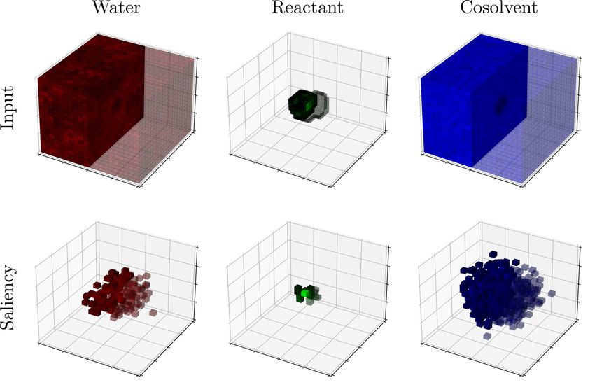
5.4 Saliency Maps
Saliency maps is a useful technique used to determine features that best explain a prediction; in
other words, these techniques seek to highlight what the CNN searches for in the data. The most
basic version of the saliency map is based on gradient information for the loss (with respect to the
input data) [30]. Recall that the forward propagation function is given by F (V; θ), where the input is
V ∈ RnV ×nV ×p , and the parameter vector is θ. We express the loss function as L (F (V; θ)) (for input
sample V); the saliency map is a tensor S ∈ RnV ×nV ×p of the same dimension as the input V and is
given by:
∂L (F (V; θ))
S = abs . (50)
∂V
If we are only interested in the location of the most important regions, we can take the maximum
value of S over all channels p and generate the saliency mask S ∈ RnV ×nV (a matrix). In some cases,
we can also study the saliency map for each channel, as this may have physical significance. Saliency
maps are easy to implement (can be obtained via back-propagation) but suffer from vanishing gra-
dients effects. The so-called integrated gradient (IG) seeks to overcome vanishing gradient effects [34];
the IG is defined as:
Z 1 !
∂L F V̄ + β V − V̄ ; θ
SIG = abs V − V̄ · dβ , (51)
0 ∂V
22http://zavalab.engr.wisc.edu
where V̄ is a baseline input that represents the absence of a feature in the input V. Typically, V̄ is a
sparse object (few non-zero entries).
6 Applications
CNNs have been applied to different problems arising in chemical engineering (and related fields)
but have been applied mostly to image data. In this section, we present different case studies to high-
light the broad versatility of CNNs; specifically, we show how to use CNNs to make predictions from
grid data objects that are general vectors (in 1D), matrices (in 2D), and tensors (in 3D). Our discussion
also seeks to highlight the different concepts discussed. The scripts to reproduce the results for the
optimal control (1D), the multivariate process monitoring (2D) and the molecular simulations (3D)
case studies can be found here https://github.com/zavalab/ML/tree/master/ConvNet.
6.1 Optimal Control (1D)
Optimal control problems (OCP) are optimization problems that are commonly encountered in engi-
neering. The basic idea is to find a control trajectory that drives a dynamical system in some optimal
sense. A common goal, for instance, is to find a control trajectory that minimizes the distance of the
system state to a given reference trajectory. Here, we study nonlinear OCPs for a quadrotor system
[11]. In this problem, we have an inverted pendulum that is placed on a quadrotor, which is required
to fly along a reference trajectory. The governing equations of the quadrotor-pendulum system are:
d2 X
= a (cos γ sin β cos α + sin γ sin α)
dt2
d2 Y
= a (cos γ sin β sin α − sin γ cos α)
dt2
d2 Z
= a cos γ cos β − g
dt2 (52)
dγ
= (ωX cos γ + ωY sin γ) / cos β
dt
dβ
= −ωX sin γ + ωY cos γ
dt
dα
= ωX cos γ tan β + ωY sin γ tan β + ωZ .
dt
where X, Y, Z are the positions and γ, β, α are angles. We define v = (X, Ẋ, Y, Ẏ , Z, Ż, γ, β, α) as state
variables, where Ẋ, Ẏ , Ż are velocities. The control variables are u = (α, ωX , ωY , ωZ ), where α is the
vertical acceleration and ωX , ωY , ωZ are the angular velocities of the quadrotor fans. Our goal is to
find a control trajectory that minimizes the cost:
T
1 2 1
Z
y = min v(t) − v ref (t) + ku(t)k2 dt, (53)
u,v 0 2 2
where v ref is a time-varying reference trajectory (changes every 30 seconds) and uref is assumed to be
zero. Minimization of this cost seeks to keep the quadrotor trajectory close to the reference trajectory
23http://zavalab.engr.wisc.edu
with as little control action (energy) as possible. An example reference trajectory v ref is shown in
Figure 12; here, we show the reference trajectories for X, Y and Z and the trajectories for the rest of
the states are assumed to be zero.
In this case study, we want to train a 1D CNN to predict optimal cost values y based on a given
reference trajectory v ref for the states (without the need of solving the OCP). This type of capability
can be used to determine reference trajectories that are least/most impactful on performance (i.e.,
trajectories that are difficult or easy to track). To train the CNN, we generated 200 random trajectories
v ref and solved the corresponding OCPs. Each OCP was discretized, modeled with JuMP [7], and
solved with IPOPT [36] [1]. After solving each OCP, we obtained the optimal states and controls v
and u (shown in Figure 12) and the optimal cost y.
Figure 12: Grid representation of time-series data. (a) Reference time-series data of state variable
X, Y and Z. The variables are normalized with a zero mean and a unit variance. Other reference
state variables Ẋ, Ẏ , Ż, γ, β and α are all zero. (b) A 240 × 9 image, where the row dimension is the
number of state variables and the column dimension is the number of time points. Each row of the
image represents one of the time series in (a). (c) Optimal solution for state variables. (d) Optimal
solutions for control variables.
The cost is the output of the 1D CNN; to obtain the input, we need to represent the reference
trajectory v ref (which includes multiple state variables) as a 1D grid object that the CNN can analyze.
Here, we represent v ref as a multi-channel 1D grid object. The data object is denoted as V; this object
24You can also read