Coupled afterslip and viscoelastic flow following the 2002 Denali Fault, Alaska earthquake
←
→
Page content transcription
If your browser does not render page correctly, please read the page content below

Geophys. J. Int. (2009) 176, 670–682                                                                           doi: 10.1111/j.1365-246X.2008.04029.x
GJI Geodesy, potential field and applied geophysics

                                                     Coupled afterslip and viscoelastic flow following the 2002 Denali
                                                     Fault, Alaska earthquake

                                                     Kaj M. Johnson,1 Roland Bürgmann2 and Jeffrey T. Freymueller3
                                                     1 Department of Geological Sciences, Indiana University, IN, USA. E-mail: kajjohns@indiana.edu
                                                     2 Department of Earth and Planetary Science, University of California, Berkeley, CA, USA
                                                     3 Department of Geology and Geophysics, University of Alaska, Fairbanks, AK, USA

                                                     Accepted 2008 November 4. Received 2008 November 4; in original form 2008 May 20

                                                                                            SUMMARY
                                                                                            Models of postseismic deformation following the 2002 M 7.9 Denali Fault, Alaska earthquake
                                                                                            provide insight into the rheologic structure of the Alaskan lithosphere and the physical pro-
                                                                                            cesses activated following a large earthquake. We model coseismic GPS displacements and

                                                                                                                                                                                                              Downloaded from http://gji.oxfordjournals.org/ by guest on February 4, 2015
                                                                                            4 yr of postseismic GPS position time-series with a coupled model of afterslip on the fault in
                                                                                            the lithosphere and distributed viscous flow in the asthenosphere. Afterslip is assumed to be
                                                                                            governed by a simplified version of a laboratory-derived rate-strengthening friction law that
                                                                                            is characterized with a single parameter, σ (a − b), where σ is the effective normal stress on
                                                                                            the fault and a − b is a dimensionless empirical parameter. Afterslip is driven by coseismic
                                                                                            stress changes on the fault generated by the main shock. The lithosphere is modelled as an
                                                                                            elastic plate overlying a linear, Maxwell, viscoelastic asthenosphere. We devise a scheme to
                                                                                            simultaneously estimate the distributions of coseismic slip and afterslip, friction parameters,
                                                                                            lithosphere thickness and asthenosphere viscosity. The postseismic GPS time-series are best
                                                                                            reproduced with a 45–85 km thick elastic lithosphere overlying an asthenosphere of viscosity
                                                                                            0.6–1.5 × 10¹⁹ Pa s. The 45–85 km elastic lithosphere thickness is greater than or equal to
                                                                                            the average crustal thickness in the region suggesting that distributed postseismic flow occurs
                                                                                            largely within the mantle while postseismic deformation in the crust is confined largely to
                                                                                            slip on a discrete fault penetrating the entire crust and perhaps into the uppermost mantle. For
                                                                                            typical laboratory values of a − b of order 10−2 at temperatures corresponding to the inferred
                                                                                            depth of afterslip, the estimated effective normal stress on the fault is ∼50 MPa, which is
                                                                                            about an order of magnitude lower than effective normal stresses at hydrostatic pore pressure.
                                                                                            Previous studies showed that models with linear Newtonian rheology cannot reproduce the
                                                                                            observed GPS time-series but that models incorporating non-linear or biviscous flow of the
                                                                                            mantle do fit the data. We show that a model with afterslip governed by a non-linear fault zone
                                                                                            rheology coupled to Newtonian mantle flow is sufficient to reproduce the GPS time-series.
                                                                                            Key words: Satellite geodesy; Transient deformation; Friction; Dynamics and mechanics of
                                                                                            faulting; Rheology: crust and lithosphere; Rheology and friction of fault zones.

                                                                                                                                    quake ruptured three fault segments shown in Fig. 1 including the
                                                     1 I N T RO D U C T I O N
                                                                                                                                    Susitna Glacier thrust and the Denali and Totschunda right-lateral
                                                     Measurements of transient deformation following earthquakes can                strike–slip faults. The Denali Fault is a large active intraplate fault
                                                     be used to probe the rheologic structure of the lithosphere. GPS               that accommodates westward rotation of the crustal block bounded
                                                     measurements of the temporal evolution of positions of points on               by the Aleutian megathrust to the south and the Denali Fault to the
                                                     the surface of the Earth have been utilized to identify multiple de-           north.
                                                     formation processes following earthquakes including viscous flow                  Previous studies demonstrate that at least two deformation mech-
                                                     in the lower crust and/or upper mantle, afterslip at crustal depths            anisms are needed to explain the Denali postseismic GPS data and
                                                     on the fault, and poroelastic response to fluid flow in the crust              that flow in the mantle below at least 40 km depth contributes sig-
                                                     (see Bürgmann & Dresen 2008, for a review). The 2002 Denali                   nificantly to the observed postseismic surface deformation. Pollitz
                                                     Fault, Alaska earthquake and 4 yr of continued postseismic defor-              (2005) showed that the GPS time-series positions for the first 1.5 yr
                                                     mation were well recorded with campaign and continuous GPS data                following the earthquake are consistent with viscous flow below
                                                     (e.g. Freed et al. 2006b) that allow us to infer rheologic properties          an elastic upper crust assuming a two-component biviscous rhe-
                                                     of the central and southern Alaskan lithosphere. The Denali earth-             ology (Burgers body) for the mantle characterized by steady-state

                                                     670                                                                                                                              C 2009 The Authors

                                                                                                                                                                           Journal compilation
                                                                                                                                                                                               C 2009 RAS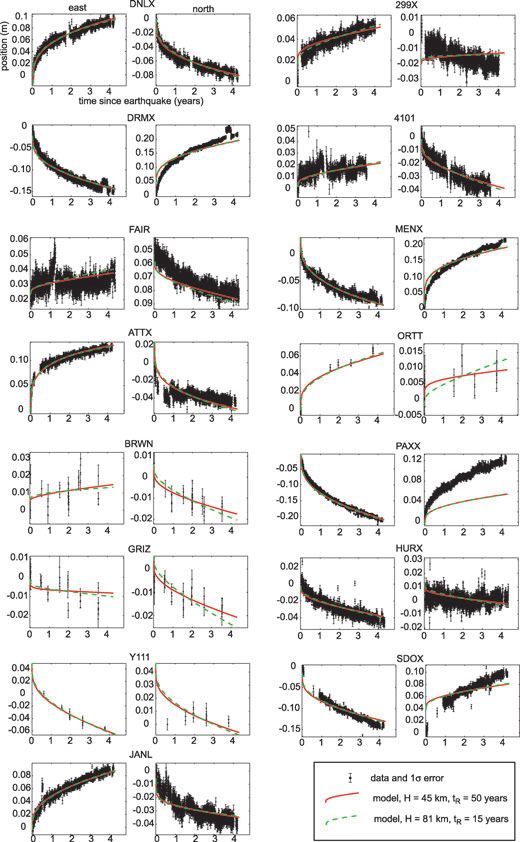
Coupled afterslip and viscoelastic flow               671

                                                                                                                                                                  Downloaded from http://gji.oxfordjournals.org/ by guest on February 4, 2015
Figure 1. Tectonic setting after Eberhart-Phillips et al. (2006) showing inferred extent of Pacific and Yakutat slab and depth contours of the plate interface.
The Denali Fault earthquake ruptured the Susitna Glacier thrust and sections of the Denali and Totschunda Faults.

viscosity of 2.8 × 10¹⁸ Pa s and a transient viscosity of 1.0 ×                    that, as suggested by Freed et al. (2006a), combined mechanisms
1017 Pa s. Pollitz (2005) modelled the lower crust as a single-                    of afterslip and deep viscous flow are needed to explain the GPS
component (Maxwell) viscous layer between 15 and 40 km depth                       data. We also show that a non-linear viscous or biviscous rheology
with viscosity of order 1019 Pa s. Freed et al. (2006a) showed that                for the mantle is not required by the data; flow of a linear Maxwell
significant postseismic flow below a depth of about 60 km is re-                   viscous mantle coupled to rate-strengthening afterslip is sufficient
quired to explain the displacements of GPS sites located far from                  to explain the observations.
the fault. Freed et al. (2006b) showed that the GPS time-series data
cannot be explained with flow of a Newtonian viscous mantle but
can be explained by flow of a mantle with non-linear, power-law de-
                                                                                   2 D ATA
pendence of strain rate on stress. Freed et al. (2006a) showed that the
GPS data and models cannot distinguish between distributed lower                   The GPS time-series used here span the time from the day after
crustal flow (between 30 and 60 km depth) and localized afterslip                  the earthquake (2002 November 4) through the end of 2007 March,
on the fault, but it is clear from Freed et al. (2006b) that shallow               approximately 4.5 yr after the earthquake. Each day of GPS data
afterslip (less than 30 km depth) on the fault is required to fit the              from sites in Alaska and the surrounding area was analysed using the
displacements at sites nearest the fault. The main conclusions from                GIPSY-OASIS version 4 software and the JPL non-fiducial orbits.
these studies regarding the rheology of the Alaskan lithosphere in-                Details of the data analysis are given in Freymueller et al. (2008).
clude: (1) flow in the mantle below at least 40 km depth is required               Each daily solution is then transformed into the ITRF2000 reference
to explain the motions of sites located far from the fault (>100 km);              frame (IGb00 realization) using roughly 20 sites distributed across
(2) a shallower source (likely afterslip) in the crust is necessary to             about 25 per cent of the surface of the Earth. This results in time-
explain motions of sites near the fault; (3) it is not possible to repro-          series of station positions in ITRF2000.
duce the observed GPS time-series either near or far from the fault                   Because we are interested primarily in modelling the transient be-
with models consisting of strictly Newtonian rheology (mantle flow                 haviour following the earthquake, we modified the post-earthquake
and/or flow within a crustal viscous shear zone) and (4) the GPS                   time-series by subtracting the pre-earthquake velocity of the site
time-series at sites far from the fault can be reproduced with models              from the post-earthquake time-series, giving a time-series that
consisting of flow in a non-linear, power-law viscous mantle or a                  should reflect only the transient deformation. We used the pre-
linear biviscous body.                                                             earthquake velocities of Freymueller et al. (2008) for sites that
   None of the above studies attempt to match GPS time-series data                 were measured before and after the earthquake. In some cases, we
with models that incorporate the coupled processes of afterslip and                have extensive post-earthquake observations from sites that had no
distributed viscous flow. Here, we investigate the relative contri-                pre-earthquake data, or only limited pre-earthquake data. In such
butions of afterslip on the fault and viscous flow in the mantle to                cases, we used either the pre-earthquake velocity of a nearby site,
the observed GPS time-series for 4 yr following the 2002 Denali                    or interpolated between sites, or used the estimated velocity based
earthquake. We model postseismic deformation with afterslip on                     on a tectonic model. The model used for this is an updated version
a fault in an elastic upper crust coupled to distributed flow in a                 of the model presented in Fletcher (2002). We only used time-series
linear Maxwell viscoelastic lower crust and/or upper mantle. The                   from sites where we could determine a pre-earthquake velocity with
afterslip is governed by a rate-strengthening friction law. We show                an estimated precision of better than 3–4 mm yr−1 . Because the


C 2009 The Authors, GJI, 176, 670–682
Journal compilation
                    C 2009 RAS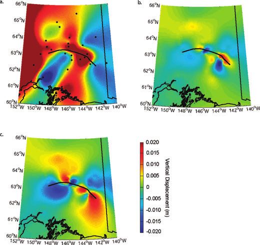
672      K. M. Johnson, R. Bürgmann and J. T. Freymueller

postseismic deformation for most sites is an order of magnitude                     by coseismic slip are then relaxed by localized afterslip on the fault
more rapid, this represents only a small error in the time-series data.             and distributed viscous flow at depth. We assume that afterslip is
   The main advantage of this approach is that it frees us from                     governed by a rate-strengthening friction law that relates the strike-
having to model the complex deformation of much of southern                         parallel shear stress, τ , and normal stress, σ , on the fault to the
Alaska. The pre-earthquake velocities in southern Alaska result                     strike-parallel component of slip rate, v,
from the superposition of several separate deformation sources
                                                                                    τ = σ {μ + (a − b) ln(v/v ∗ )} ,                                          (1)
(Freymueller et al. 2008), and by removing the pre-earthquake
velocities we need only to model what has changed as a re-                          where μ is the nominal coefficient of friction, v ∗ is a reference
sult of the earthquake. We make the assumption here that all                        sliding velocity and a − b is a dimensionless friction parameter that
of the pre-earthquake deformation sources do not change with                        is found in lab experiments to be typically of order 10−3 to 10−2 .
time, except for the afterslip and viscoelastic relaxation model                    This formulation is a simplified version of a more general rate-
described in the next section. We later relax that assumption                       and-state-dependent frictional behaviour inferred from laboratory
by estimating an additional component in the model due to                           experiments (e.g. Dieterich 1981) that has also been adopted by a
changes in the slip deficit distribution on the subducting plate                    number of previous afterslip studies (e.g. Marone et al. 1991; Linker
interface.                                                                          & Rice 1997; Hearn et al. 2002; Perfettini & Avouac 2007a).
                                                                                        We need the stress on a patch at any time to compute the slip
                                                                                    rate using eq. (1). Let g i (t − t 0 ) be a 1 × m vector of Green’s
3 MODEL AND INVERSION
                                                                                    functions that relates the shear stress, τ i , on the ith patch at time
                                                                                    t to unit slip on m patches at time t 0 . The g i are time-dependent
3.1 Afterslip model
                                                                                    because viscous flow in the asthenosphere varies with time. The

                                                                                                                                                                     Downloaded from http://gji.oxfordjournals.org/ by guest on February 4, 2015
We idealize the Alaskan lithosphere and asthenosphere with a ho-                    g i are computed using semi-analytical propagator matrix methods
mogeneous elastic plate overlying a Maxwell viscoelastic half-space                 (e.g. Fukahata & Matsu’ura 2006). Let τ ic (t) be the shear stress
with uniform viscosity, η, and shear modulus, μ (uniform relaxation                 induced on the ith patch by coseismic slip and associated viscous
time, t R = 2η/μ) as illustrated in Fig. 2. The fault cuts through the              flow. Then, the stress on the ith patch at time t, due to coseismic
entire elastic plate but does not penetrate into the viscoelastic sub-              slip and postseismic slip-rate history v (t), where v (t) is a m × 1
strate. The fault is discretized into 5.5 × 1.5 km rectangular patches.             vector of slip rates, is
For now, we ignore the complexities introduced by the presence of                                      t
the subducting slab and lateral variations in crustal properties, but               τi (t) = τi (t) +
                                                                                               c
                                                                                                          gi (t − t  )v(t  ) dt  .                    (2)
in the discussion we address the possible influences of these lateral                                  0

variations on our results.                                                          We approximate the integral by discretizing time into N discrete
   For simplicity, we only consider the strike–slip component of                    steps with duration δ 1 , δ 2 , . . . , δ N where N and δ k will be determined
fault slip. To induce coupled afterslip and viscoelastic flow, we                   in the integration scheme. Stress and slip rate is computed at the
impose coseismic slip on fault patches above 18 km depth. The                       midpoint of timeincrements. The midpoint of the jth time increment
                                                                                                       j−1
stresses on the fault and within the viscoelastic substrate induced                 is t j = 0.5δ j + k=1    δk . Then, the stress on the ith patch during the

Figure 2. Illustration of model showing discretized fault surface in elastic lithosphere overlying viscoelastic asthenosphere. Coseismic slip is allowed to occur
from the surface to 18 km depth. The entire discretized fault surface is allowed to creep following the earthquake. The velocity-strengthening slip law is
employed to model afterslip. Uniform frictional properties are assigned to the fault.


                                                                                                                       C   2009 The Authors, GJI, 176, 670–682
                                                                                                                               Journal compilation
                                                                                                                                                   C 2009 RAS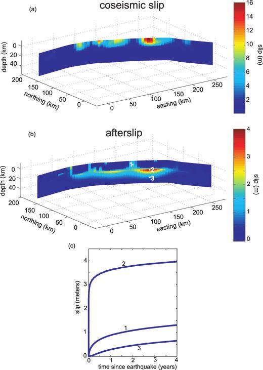
Coupled afterslip and viscoelastic flow              673

jth time increment is                                                            is assumed to be a diagonal matrix). We conduct the traditional slip
                                                                                 inversion by minimizing the objective function

                           j−1
τi (t j ) ≈ τic (t j ) +         gi (t j − tk )sk ,                       (3)            −1/2
                                                                                 1 = ||co           −1/2
                                                                                              Gsco − co   dco ||2 + γ 2 ||∇ 2 sco ||2 ,   sco ≥ 0,     (7)
                           k=1
                                                                                 where ∇ 2 is the discrete Laplacian operator, || || denotes the L-2
where the s k are m × 1 vectors of average slip during the kth time              norm and s co ≥ 0 indicates that slip is constrained to be right-lateral
step. We assume that the fault is slipping at steady-state velocity, v 0 ,       (positive). This is the standard damped least-squares inversion with
before the earthquake. Fletcher (2002) and Matmon et al. (2006)                  positivity constraints for slip, where γ is a so-called smoothing
estimated a slip rate of 0.008–0.012 m yr−1 for the Denali Fault,                parameter that determines the relative weight placed on fitting the
so we assume v 0 = 0.01 m yr−1 for depths greater than 18 km and                 data versus smoothing the coseismic slip distribution (e.g. Du et al.
v 0 = 10−4 m yr−1 (effectively, locked) for depths less than 18 km.              1992).
Letting v ∗ in eq. (1) be equal to v 0 , such that the initial stress before        For the postseismic part of the problem, we assume that the time-
the earthquake is τ 0 = σ μ, then from eq. (1), the average afterslip            series positions of GPS sites relative to pre-earthquake positions,
rate on the ith patch during the jth time interval is                            d post (t), are related to afterslip on the fault (total accumulated slip
                                                                               minus slip accumulated at the pre-earthquake rate), s post (t), coseis-
                     τi (t j ) − τ0
vi (t j ) = v0 exp                    ,                                  (4)     mic slip, s co , and surface displacements associated with distortion
                      σ (a − b)
                                                                                 of the elastic crust coupled to flow in the mantle, d visco (t), through
where τ i (t j ) is given by eq. (3). Here, v > 0 indicates right-lateral        the observation equation,
sense of slip. It is clear from eq. (4) that τ > τ 0 generates slip
at a higher rate than v 0 and τ < τ 0 generates slip at a lower rate             dpost (t) = doffset + Gsco + dvisco (t) + Gspost (t)
than v 0 . Eq. (4) does not permit left-lateral slip and therefore areas                    +     (ψ1 , ψ2 , ψ3 , ψ4 ) + post ,

                                                                                                                                                               Downloaded from http://gji.oxfordjournals.org/ by guest on February 4, 2015
                                                                                                                                                        (8)
of the fault that slip coseismically and experience a drop in shear
                                                                                 where G is the same kernel matrix as in (6) and d offset is a vector
stress will essentially stop sliding following the earthquake. The slip
                                                                                 of constants that account for unknown pre-earthquake positions for
during the jth time interval on the ith patch is determined by a simple
                                                                                 campaign sites or new continuous GPS sites that do not have mea-
numerical integration, s i (t j ) = v i (t j ) δ j , where the duration of the
                                                                                 surements before the earthquake. The data errors,  post , are assumed
time interval, δ j , is inversely proportional to v i (t j ) and is tuned to
                                                                                 to be Gaussian with covariance matrix,  post (this is assumed to be
give sufficient integration accuracy. Let s (t j ) be the m × 1 vector of
                                                                                 a diagonal matrix).     is a vector of sinusoidal terms that model
average slip on all m patches during the jth time increment. Because
                                                                                 non-tectonic seasonal variations in the time-series positions of con-
we have removed a pre-earthquake trend from the GPS time-series
                                                                                 tinuous GPS sites
data, we compute the slip during the jth time interval in excess of
the slip that would accumulate at the pre-earthquake slip rate,                    (ψ1 , ψ2 , ψ3 , ψ4 ) = ψ1 sin(2π t) + ψ2 cos(2π t)

spost (t j ) = s(t j ) − v0 δ j .                                         (5)                             + ψ3 sin(4π t) + ψ4 cos(4π t),                (9)
                                                                                 where the ψ i are different for each continuous GPS site and both east
We emphasize that although s post is strictly postseismic slip that
                                                                                 and north components. This is a standard approach for accounting
occurs in excess of the pre-earthquake slip rate, s post does depend
                                                                                 for unknown cyclic fluctuations in GPS measurements (e.g. Freed
on the interseismic slip rate, v 0 and shear stress, τ 0 , through eq. (4).
                                                                                 et al. 2006a).
   In this model, the entire fault is assumed to be velocity-
                                                                                    Eq. (8) is a highly non-linear relationship between the observ-
strengthening and is assigned uniform value of σ (a − b). Any
                                                                                 ables, d post (t), and the model parameters because: (1) s co depends
part of the fault that experiences a large coseismic shear stress in-
                                                                                 non-linearly on γ ; (2) s post (t) depends non-linearly on s co , σ μ,
crease will slip rapidly following the earthquake and regions the
                                                                                 σ (a − b), H and t R and (3) d visco (t) depends in turn on s co and s post
slip coseismically will experience a large shear stress decrease and
                                                                                 as well as non-linearly on H and t R . We seek values of these param-
effectively lock up after the earthquake. We therefore conceptual-
                                                                                 eters, through an inversion, that reproduce the observed GPS time-
ize a fault with velocity-weakening patches that are stuck during
                                                                                 series. The complete inverse solution would be the joint posterior
the interseismic period and rupture during earthquakes surrounded
                                                                                 probability distribution for all of the unknown parameters, which
by velocity-strengthening regions that creep during the interseismic
                                                                                 contains all information about the solution including the most likely
period and exhibit rapid afterslip following earthquakes. However,
                                                                                 solution and a description of the model uncertainties. However, it
we do not explicitly model the velocity-weakening patches.
                                                                                 would be computationally burdensome to estimate the posterior
                                                                                 probability distributions of the model parameters because a for-
                                                                                 ward model computation of the postseismic displacements (eq. 8)
3.2 Inversion method
                                                                                 requires computing a non-negative least-squares inversion for co-
In this work, we jointly invert coseismic and postseismic GPS data               seismic slip, a numerical computation of displacements and stresses
for coseismic slip, friction parameter, σ (a − b), elastic thickness, H,         at many time intervals using a propagator matrix code, and a nu-
and asthenosphere relaxation time, t R . The observation equation for            merical computation for the afterslip evolution with time. We take
the coseismic part of the problem relates a vector of coseismic                  a less exhaustive approach and seek a set of optimal model param-
offsets, d co , to a vector of slip on fault patches, s co ,                     eters. The optimal solution is the set of parameters that minimizes
                                                                                 the objective function
dco = Gsco + co ,                                                        (6)

where we relate slip to surface displacements through the kernel                                  −1/2
                                                                                 2 = 1 + ||post (d̂ − dpost )||2 ,                                  (10)
matrix, G, which is derived from the solution for a rectangular
dislocation in an elastic half-space (Okada 1992). The data errors,              where d̂ is a vector of predicted postseismic time-series positions
 co , are assumed to be Gaussian with covariance matrix,  co (this             and  1 is the objective function defined in (7). In the standard


C 2009 The Authors, GJI, 176, 670–682
Journal compilation
                    C 2009 RAS
674 K. M. Johnson, R. Bürgmann and J. T. Freymueller
slip-inversion method, the value for γ in the objective function, 1 , t R space, or σ (a − b) space, and then sampling the distributions
must be specified and a separate technique must be introduced to using a Monte Carlo-Metropolis algorithm (e.g. Fukuda & Johnson
select an optimal value for this parameter (e.g. Fukuda & Johnson 2008), interpolating at values between the regularly spaced values.
2008). However, following Johnson et al. (2006), we have set up this We also consider a double-exponential error model for the data, in
problem so that we simultaneously invert coseismic and postseismic which the joint posterior probability distribution is
data such that the smoothing parameter, γ , can be optimized with 1
this objective function. The objective function (10) is a function of p(α, H, tR , σ (a − b)|dpost , γ 2 ) =
(2α) N
all the unknown parameters in this problem,
−1 k
N
2 = 2 (γ , aσ, H, tR , ψ1 , ψ2 , ψ3 , ψ4 ). (11) exp |(d − d̂ k )| , (13)
2α k=1 post
We minimize the objective function, 2 , (10) using the following
procedure: (1) select a value for γ and invert coseismic GPS dis- where d kpost and d̂ k denote the kth measured and predicted time-
placements for fault slip using the standard, damped least-squares series position, respectively. The posterior distributions for fixed
slip-inversion method with positivity constraints to minimize 1 ; H and t R or σ (a − b) are determined similarly as above for the
(2) select values for σ (a − b), H and t R , compute the coseismic Gaussian error model.
stress change from the coseismic slip distribution to use as the ini-
tial stress condition for the numerical integration of (1) to obtain
the evolution of afterslip, s post (t); (3) compute the predicted surface 4 R E S U LT S
positions, Gs post (t) +d visco (t) and use least squares to invert eq. (8) The objective function (10) is minimized with values of H =
for the seasonal terms (ψ 1 , ψ 2 , ψ 3 , ψ 4 ) and offsets (d offset ) with 81 km, t R = 15 yr (corresponding to η = 6 × 10¹⁸ Pa s), and
σ (a − b) = 0.48 MPa. The estimates of the posterior probabil-
Downloaded from http://gji.oxfordjournals.org/ by guest on February 4, 2015
Gs co , d visco (t) and Gs post (t) fixed and (4) compute the value for the
objective function, 2 , (10). A minimum value for 2 is found us- ity distributions, using the method described above, are shown in
ing a simple downhill search method, computing steps 1–4 for each Fig. 3. The double-exponential and Gaussian error models for the
set of model parameters until 2 does not change within a specified data result in very different estimates of elastic thickness and re-
tolerance. laxation time, although the 95 per cent confidence regions for both
To provide an estimate of the uncertainties of the most impor- error models are relatively small. The small formal model parameter
tant posterior model parameters, we approximate the posterior joint uncertainties are probably not representative of the true uncertainty
marginal distribution of H and t R and marginal posterior distribu- in parameters, however. Fig. 4 shows the fit to the data for the best-
tion of σ (a − b). Assuming Gaussian data errors with covariance fitting models for the two data error structures. The model with
matrix, d , the posterior distribution of model parameters given N elastic thickness of 45 km and asthenosphere relaxation time of
data and fixed coseismic slip distribution (fixed γ 2 ) is 50 yr fits the data qualitatively as well as the model with an 81 km
1 thick elastic layer and asthenosphere relaxation time of 15 yr. The
p(α 2 , H, tR , σ (a − b)|dpost , γ 2 ) = formal uncertainties on model parameters as shown in Fig. 3 are
(2π α 2 ) N /2
probably excessively small because the inversion does not properly
−1 T −1
exp (d post − d̂) d (d post − d̂) , (12) take into consideration uncertainty in the earth model and perhaps
2α 2 because of systematic misfit to the data. The estimated elastic layer
where α 2 is an unknown scalar multiplier of the data variance ma- thickness of about 45–85 is similar to or larger than the average
trix and will be estimated (e.g. Fukuda & Johnson 2008). It is crustal thickness of 50 km in central Alaska (Brocher et al. 2004)
computationally intensive to estimate the distribution (12), so we suggesting that viscous flow dominantly occurs in the upper mantle
instead estimate the distributions p(α 2 , H, tR |dpost , γ 2 , σ̂ (a − b)) and not in the lower crust.
and p(α 2 , σ (a −b)|dpost , γ 2 , Ĥ , tˆR ) with H and t R or σ (a − b) fixed The coseismic slip and cumulative afterslip distributions are
to the values determined using the optimization scheme described shown in Figs 5(a) and (b) for H = 45 km and t R = 50 yr. The mag-
above (hat symbol denotes optimal value). These distributions are nitude of right-lateral slip is shown on each patch. The coseismic
estimated by first computing d̂ at regularly spaced points in H – slip is concentrated in five patches, similar to that inferred by others
Figure 3. (a) Contours of posterior probability for Gaussian and double-exponential data error models. Outer contour corresponds approximately with the
boundary of the 99 per cent confidence region. Joint distribution of relaxation time and elastic thickness assuming optimized values (Gaussian data error
model) for σ (a − b) and smoothing parameter, γ 2 . (b) Marginal posterior probability distribution for σ (a − b) assuming optimized values (Gaussian data
error model) for elastic thickness and relaxation time.
C 2009 The Authors, GJI, 176, 670–682
Journal compilation
C 2009 RASCoupled afterslip and viscoelastic flow 675
Downloaded from http://gji.oxfordjournals.org/ by guest on February 4, 2015
Figure 4. GPS time-series and 1σ errors. A pre-earthquake linear trend has been removed from the data. Axes labels are shown only for the first plot and are
the same for all plots (vertical axis is position in metres and horizontal axis is time since the earthquake in years). For each pair of plots, the east component of
position is shown on the left-hand side and the north component of position on the right-hand side. Red, solid curves show best-fitting model for the case of
Gaussian data errors. Dashed, green curves show best-fitting model for the case of double-exponential data errors. Periodic seasonal variations in the time-series
are estimated in the inversions but are not shown in the plots.
(e.g. Wright et al. 2004; Hreinsdóttir et al. 2006; Elliot et al. 2007). in Fig. 5(c). The slip on patch 2 (patch with maximum cumulative
Most of the afterslip is concentrated between 18 and 30 km depth afterslip) exhibits the most rapid afterslip in the first days following
below the three largest coseismic slip patches. Smaller amounts the earthquake, while the shallowest patch (patch 1) exhibits much
of afterslip occur at shallower depths between the coseismic slip lower slip rates during this time and afterslip on the deepest patch
patches. The inferred patches of afterslip above 18 km depth is (patch 3) actually accelerates slowly for the first 3 months before
similar to that imaged in a kinematic slip inversion in Freed et al. decelerating. After about half a year following the earthquake, the
(2006a) which shows a patch of afterslip consistent with the patch afterslip decelerates at similar rates on all three patches. After 4.5 yr,
at a distance of about 200 km from the west end of the fault in the slip rate over much of the fault below 18 km depth is about 0.009
Fig. 5(b). The time evolution of afterslip on three patches is shown m yr−1 faster than the pre-earthquake rate of 0.01 m yr−1 .
C 2009 The Authors, GJI, 176, 670–682
Journal compilation
C 2009 RAS676 K. M. Johnson, R. Bürgmann and J. T. Freymueller
Downloaded from http://gji.oxfordjournals.org/ by guest on February 4, 2015
Figure 5. Slip distributions for optimal solution determined assuming double-exponential data errors (H = 45 km, t R = 50 yr, σ (a − b) = 0.5 MPa).
(a) Coseismic slip distribution showing magnitude of right-lateral slip. Coseismic slip is constrained to depths of 0–18 km in the inversion although fault is
shown to extend to depth of 45 km. (b) 4-yr cumulative afterslip showing magnitude of right-lateral slip. Afterslip extends to the bottom of the elastic plate
(bottom of shown fault surface) and is concentrated immediately below and between large coseismic slip patches. (c) Slip evolution with time on three patches
labelled in (b).
The fit to the time-series is shown in Fig. 4 without the sinusoidal side of the Denali Fault are fit within the 2σ error ellipses, but there
seasonal terms. The fit is generally better in the east component are significant misfits on the southern side of the fault. As men-
than the north component. Most of the east component time-series tioned above, the misfit is especially large in the north component
positions are fit within the uncertainties. There is a systematic misfit of the displacements such as seen at sites clustered near latitude
in the north component that we discuss below. The observed high 62◦ N. Significant misfits near the Totschunda segment (between
surface velocities in the first few months after the earthquake and the 142◦ and 144◦ W and 62◦ and 63◦ N) may be due to mismodelled
lower velocities at later times are reproduced well at both near-fault shallow afterslip. It is important to note that although it is illustra-
sites (e.g. DNLX) and sites far from the fault (e.g. FAIR). However, tive to look at the residuals in Fig. 6, we did not minimize the misfit
the rapid postseismic signal in the first few months is underpredicted between observed and computed cumulative displacements, rather,
at a few of the sites located 100–300 km from the fault (e.g. sites we modelled the time-series positions.
299X and 4101) suggesting a possible missing postseismic source We did not invert the vertical component of GPS data because
in our model such as afterslip deeper on the fault or distributed, the vertical time-series are relatively noisy and there are system-
non-linear viscous flow at depth (Freed et al. 2006b). atic misfits between the vertical displacements and postseismic
Fig. 6 shows the observed and computed cumulative 4-yr post- models (e.g. Freed et al. 2006a, fig. 17), suggesting that hydro-
seismic displacements. Most of the displacements on the northern logic, ice-unloading, or other processes not considered in our study
C 2009 The Authors, GJI, 176, 670–682
Journal compilation
C 2009 RASCoupled afterslip and viscoelastic flow 677
Downloaded from http://gji.oxfordjournals.org/ by guest on February 4, 2015
Figure 6. Observed and predicted cumulative 4-yr postseismic displacements. Time-series for labelled sites are shown in Fig. 4. Box north of fault outlines
sites used for profile in Fig. 9.
may contribute to the vertical motions. We show a smoothed, con- different at the farthest sites (FAIR and 4101). Fig. 9 also plots the
toured version of the measured cumulative vertical displacements cumulative, 4 yr displacements at sites located in the box north of
in Fig. 7(a) along with model predictions of the vertical displace- the fault shown in Fig. 6. Both models systematically underpredict
ments. The displacements in Fig. 7 are relative to site WHIT which cumulative displacements and the afterslip-only model underpre-
is located in western Canada (just east of the figure). Fig. 7(b) shows dicts displacements slightly worse than the coupled afterslip/flow
the predicted vertical displacements for the optimized coupled after- model.
slip/flow model. Fig. 7(c) combines the optimized predicted vertical
displacements with the predicted vertical displacements in a fully
drained poroelastic half-space (assuming ν = 0.29 and 0.25 for
5 DISCUSSION
undrained and drained Poisson’s ratio, respectively). Although the
correspondence between the smoothed vertical displacement field For typical laboratory values of a − b of order 10−2 at temperatures
in Fig. 7(a) and the prediction in Fig. 7(c) is not exact, the pat- corresponding to depths greater than 18 km (e.g. Blanpied et al.
terns are similar with a four-quadrant distribution of uplifted and 1995), our estimate of σ (a − b) = 0.48 implies effective normal
subsided regions. stress of about 50 MPa which is lower than effective normal stress
Fig. 8 shows the fit to the data for H = 45 km and t R = 50 yr of 360–800 MPa under hydrostatic pore pressures between 18 and
with and without the contribution to surface displacements from 40 km depth. Therefore, either the value of a − b for the Denali
viscous flow in the asthenosphere. The predicted time-series for the Fault is about an order of magnitude lower than laboratory values or
case without the contribution from viscous flow is simply computed elevated pore pressure in the fault zone reduces σ (a − b). This value
by setting the term d visco (t) in eq. (8) equal to zero. The compar- of σ (a − b) is comparable to values obtained using similar models
ison illustrates the relative contributions to surface displacement of afterslip for other earthquakes. Hearn et al. (2002) estimated a
from mantle flow and afterslip. The contribution to surface dis- value of 0.2–0.4 MPa using postseismic data from the 1999 Izmit,
placement from deep viscous flow is insignificant at sites near the Turkey earthquake and Perfettini & Avouac (2007a) estimated a
fault (e.g. ATTX, Fig. 6) and small but significant at sites far from value of 0.5 MPa using postseismic data from the 1992 Landers,
the fault (e.g. FAIR and 4101, Fig. 6). California earthquake. Several other studies also infer values of
Fig. 9 shows the fit to the data for the case H = 45 km and σ (a − b) in the range 0.2–0.7 MPa from postseismic geodetic data
t R = 50 yr and for a the best-fitting model with afterslip only (no (Miyazaki et al. 2004; Hsu & Bock 2006; Perfettini & Avouac
viscous flow in the asthenosphere). The afterslip-only inversion was 2007b). Consistent with our estimate of small σ , Wesson & Boyd
conducted by minimizing the objective function (10) using eq. (8) (2007) infer low absolute shear stress (1–4 MPa) at a depth of about
without the term d visco (t). The fit is nearly identical for the two mod- 5 km in the vicinity of the Denali Fault using stress tensor inversion
els at the two sites nearest the fault (DNLX and JANL) and slightly of focal mechanisms before and after the Denali Fault earthquake.
C 2009 The Authors, GJI, 176, 670–682
Journal compilation
C 2009 RAS678 K. M. Johnson, R. Bürgmann and J. T. Freymueller
Downloaded from http://gji.oxfordjournals.org/ by guest on February 4, 2015
Figure 7. (a) Contoured 4-yr cumulative vertical displacements measured with GPS. Displacements are relative to site WHIT which is located in western
Canada. Contour algorithm forces the surface to go through data (block dots) and interpolates between points with splines. (b) Modelled vertical displacements
assuming H = 45 km and t R = 50 yr. (c) Same as (b) but with additional vertical displacement predicted by a model for a fully drained poroelastic half-space.
The observed gross uplift/subsidence pattern is similar to the predicted pattern and the magnitude of uplift/subsidence is better predicted in (c) with the
additional contribution from poroelasticity.
Assuming a coefficient of friction of 0.6, the 1–4 MPa shear stress is terslip/viscous flow model that incorporates non-linear or biviscous
consistent with an effective normal stress on the fault at 5 km depth asthenosphere flow could reproduce the data with a larger contri-
of less than 10 per cent of the lithostatic load minus hydrostatic pore bution from viscous flow. The plot of cumulative displacements
pressure, similar to our independent estimate. with distance from the fault in Fig. 9 shows that both the coupled
There is much discussion in the literature regarding the nature of afterslip/viscous flow model and the afterslip-only model systemat-
deformation in the lower crust. For example, there is evidence that ically underpredict displacements. The afterslip-only model under-
the lower crust deforms as a broad zone of distributed shear and other predicts cumulative displacements slightly worse than the coupled
evidence that deformation in the crust is largely confined to narrow model indicating that the additional contribution of asthenosphere
shear zones that are the ductile downward extension of brittle faults flow to surface displacements improves the fit some. The systematic
in the upper crust (e.g. Bürgmann & Dresen 2008). Unfortunately, underprediction of displacements might be reconciled with a con-
it is not yet possible to distinguish between these two possibilities tribution to surface displacements from flow in the asthenosphere
for the Alaskan crust using only postseismic data from the Denali of a material with an effective viscosity that varies with time.
Fault earthquake. Our results demonstrate that horizontal postseis- Although the general patterns observed in the time-series and
mic GPS time-series data are consistent with models in which lower cumulative displacements are reproduced well in a qualitative sense
crustal deformation is confined to afterslip on a discrete fault or by this fairly simple model of postseismic deformation, there is a
narrow shear zone. However, Freed et al. (2006b) demonstrate that systematic, asymmetric pattern of misfit shown in Fig. 10 between
these data are also consistent with models of distributed flow in the the measured 4-yr cumulative postseismic displacements and the
lower crust without afterslip on a discrete, through-going fault in model. On the north side of the Denali Fault, the residual vectors
the lower crust. This ambiguity has arisen in models of postseis- are mostly within the 2 σ uncertainty ellipses and nearly randomly
mic deformation following other large earthquakes. For example, oriented. But on the south side of the Denali Fault, the residual
postseismic deformation of the lower crust following the Landers, displacements are systematically oriented to the northwest, similarly
California earthquake has been attributed to afterslip (e.g. Savage to the plate convergence direction (Fig. 1). As our data set has
& Svarc 1997; Fialko 2004) and distributed viscous flow (e.g. Deng been corrected for interseismic deformation based in large part on
et al. 1998). GPS rates determined at these sites during the years prior to the
Our inversions attribute most of the postseismic signal to afterslip earthquake, this cannot be attributed to background elastic plate
on the fault. However, models with non-linear (Freed et al. 2006b) boundary strain.
or biviscous (Pollitz 2005) asthenosphere viscosity can reproduce We consider the possibility that lateral variations in
time-series observations at far-field sites. Presumably a coupled af- crustal/lithosphere rheology could account for the observed
C 2009 The Authors, GJI, 176, 670–682
Journal compilation
C 2009 RASCoupled afterslip and viscoelastic flow 679
Downloaded from http://gji.oxfordjournals.org/ by guest on February 4, 2015
Figure 8. GPS time-series and 1σ errors. A pre-earthquake linear trend has been removed from the data. Axes labels are shown only for the first plot and are
the same for all plots (vertical axis is position in metres and horizontal axis is time since the earthquake in years). For each pair of plots, the east component
of position is shown on the left-hand side and the north component of position on the right-hand side. Plot compares model prediction with and without the
contribution to surface displacements from viscous flow in the asthenosphere. Red, solid curves show best-fitting coupled afterslip/viscous flow model for the
case of Gaussian data errors. Dashed, green curves show predictions from the same model, but without the contribution to surface displacements from viscous
flow. Periodic seasonal variations in the time-series are estimated in the inversions but are not shown in the plots.
asymmetric pattern in surface displacements. The subducting slab tions using a boundary element technique. We extend the popular
beneath southern Alaska is one obvious source of lateral varia- displacement-discontinuity boundary element method for elasticity
tion in lithosphere structure (e.g. Eberhart-Phillips et al. 2006). (e.g. Crouch & Starfield 1983) to incorporate linear Maxwell vis-
Also, tomographic inversions by Eberhart-Phillips et al. (2006) in- coelastic domains. Figs 11(a) and (b) show the assumed geometry
dicate that the crust is thicker on the southern side of the Denali for the two cases and Fig. 11(c) shows the velocity profiles across
Fault than the northern side. We constructed simplified 2-D models the fault. In the model, we impose 6 m of sudden slip on the locked
of a strike–slip fault that crudely incorporate these lateral varia- portion of the fault and allow the viscoelastic substrate below to
C 2009 The Authors, GJI, 176, 670–682
Journal compilation
C 2009 RAS680 K. M. Johnson, R. Bürgmann and J. T. Freymueller
east DNLX north FAIR
east north
0.10 0 0.06
displacement (m)
displacement (m)
-0.01
-0.02 0.05
-0.02
0.05 -0.04 0.04
-0.03
-0.06 0.03
-0.04
0 -0.08 0.02
-0.05
0 1 2 3 4 0 1 2 3 4 0 1 2 3 4 0 1 2 3 4
time since earthquake (years) time since earthquake (years)
JANL 0.16
0
0.08
0.14
0.06 -0.01 DNLX
displacement (m)
0.04 -0.02 0.12
coupled afterslip/flow
0.02 -0.03
0.10 JANL afterslip only
0 -0.04
0 1 2 3 4 0 1 2 3 4
0.08
4101
0.05 0.06
0
0.04 4101
-0.01 FAIR
0.03 0.04
0.02 -0.02
0.01 -0.03 0.02
0 -0.04
0
0 1 2 3 4 0 1 2 3 4 0 50 100 150 200 250 300
distance from fault (km)
Figure 9. GPS time-series and 1σ errors for selected sites within the box in Fig. 6. Red, solid curves show best-fitting coupled afterslip/viscous flow model for
Downloaded from http://gji.oxfordjournals.org/ by guest on February 4, 2015
the case of Gaussian data errors. Dashed, green curves show best-fitting model assuming no asthenosphere flow (afterslip only) for the case of Gaussian data
errors. Also shown is plot of observed and predicted cumulative 4 yr displacements at sites within the box in Fig. 6. Both models systematically underpredict
the cumulative displacements.
cannot account for the observed asymmetry in the displacement
residuals.
The residual displacement field actually resembles the interseis-
mic velocity field in this region (e.g. Ohta et al. 2006) due to locking
of the plate interface and accumulating elastic strain in the overrid-
ing plate. Therefore, we consider the possibility that the residuals
are due to transiently increased coupling of the plate interface. We
model interface coupling with backslip of elastic dislocations in an
elastic half-space following the now-standard approach introduced
by Savage (1983). We invert for the distribution of backslip using
the same slip-inversion scheme adopted for the coseismic slip in-
version described previously. The smoothing parameter is selected
subjectively to give a qualitatively smooth backslip distribution.
The backslip is shown in Fig. 11(d) and the fit to the residual dis-
placements is shown in Fig. 10. The fully locked region of the plate
interface inferred by Ohta et al. (2006) is shown in Fig. 11(d). Ohta
et al. (2006) infer the region immediately surrounding this fully
locked patch to be partly locked (non-zero sliding but at a rate
lower than plate convergence). The general residual displacement
pattern is reproduced by backslip on the interface in the areas sur-
rounding the fully locked patch. This result hints at the possibility
Figure 10. Black vectors are residual cumulative 4-yr displacement vectors that some of the increased velocities south of the Denali Fault fol-
(observed—model) centred on the 95 per cent data uncertainty ellipses. lowing the earthquake could be due to decreased creep rate of the
Model is the case H = 45 km and t R = 50 yr. Note the systematic misfit
plate interface below the locked section, but it is difficult to identify
pattern to the south of the fault, with residual vectors pointing to the NW,
a mechanism for such widespread reduction in creep rate. Further
suggesting a missing source of deformation. Residual vectors north of the
fault are largely within the error ellipses and randomly oriented suggesting more, the imaged backslip rate on the far right-hand side (Yakutat
the model satisfactorily accounts for this part of the signal. Heavy grey Slab, Fig. 1) is considerably higher than the plate convergence rate.
arrows show predicted surface displacements for the slip inversion shown The effect of the Denali Fault earthquake is to increase the downdip
in Fig. 11. component of shear stress on the subduction interface near 144◦ W,
61◦ N, which would promote decreased creep rate at the interface.
flow in response to the sudden load. The plots show the surface The maximum shear stress change in this region is about 50 kPa,
velocities 4 yr after the imposed earthquake. The asymmetry in the which according to spring-slider calculations with rate-state fric-
model surface displacements is opposite to the observed asymmetry tion (e.g. Johnson et al. 2006), is sufficient to cause the interface
in surface displacements. The models display higher velocities on to locally lock up for several years for a narrow range of friction
the north side of the fault, whereas the displacements (velocities) parameters. However, the shear stress changes over most of the in-
are observed to have been larger on the south side of the fault. terface are too small to generate appreciable widespread reduction
Therefore, a contrast in effective elastic thickness across the fault in creep rate.
C 2009 The Authors, GJI, 176, 670–682
Journal compilation
C 2009 RASCoupled afterslip and viscoelastic flow 681
Downloaded from http://gji.oxfordjournals.org/ by guest on February 4, 2015
Figure 11. (a) Illustration of geometry of 2-D boundary element model of a vertical strike–slip fault in elastic lithosphere with variable thickness overlying a
viscoelastic asthenosphere. (b) Illustration of 2-D boundary element model of simplified geometry of a strike–slip fault in an elastic lithosphere with variable
thickness overlying an elastic subducting slab in a viscoelastic asthenosphere. (c) Velocity profiles for 2-D models in (a) and (b) after a sudden displacement
discontinuity of 6 m is imposed on the fault. Note that the asymmetry in the predicted velocity profiles is opposite to the observed asymmetry in the residual
displacement pattern in Fig. 10. (d) Inversion for backslip on subducting plate interface. The backslip might represent reduced forward slip on the subduction
interface following the earthquake. The geometry and location of the locked asperity is from Ohta et al. (2006). Backslip is assumed to be zero within the
asperity.
6 C O N C LU S I O N S displacements while models that include mantle flow improve the
fit but still systematically underpredict cumulative surface displace-
We model coseismic GPS displacements and 4 yr of postseismic
ments. It is clear from several previous studies that the postseismic
GPS time-series positions with a coupled model of afterslip on the
GPS time-series cannot be reproduced with models incorporating
fault in the lithosphere and distributed viscous flow in the astheno-
strictly Newtonian viscosity for the mantle and/or a crustal shear
sphere. Afterslip is assumed to be governed by a laboratory-derived
zone. Previous studies showed that models that incorporate either
rate-strengthening friction law. The postseismic GPS time-series are
non-linear power-law mantle flow or linear biviscous mantle flow
best reproduced with a 45–85-km-thick elastic lithosphere overlying
can reproduce the GPS time-series at sites far enough from the fault
asthenosphere with viscosity of 0.6–1.5 × 10¹⁹ Pa s. The inferred
that are not highly influenced by shallow afterslip. Our results show
45–85 km lithosphere thickness is equal to or larger than the crustal
that it is possible that the non-Newtonian behaviour that is inferred
thickness in the region inferred from seismology suggesting that
from the GPS time-series may occur at crustal depths as afterslip
deformation in the lower crust is confined largely to slip on a dis-
within a shear zone with velocity-strengthening friction.
crete fault penetrating the entire crust with distributed viscous flow
occurring largely below the crust in the upper mantle. However, this
is not a unique result as previous studies using a shorter time span AC K N OW L E D G M E N T S
of data have shown that the postseismic GPS data can also be ex- The authors are grateful to the associate editor, Jim Savage, and
plained with distributed flow in the lower crust. For our best-fitting Hugo Perfettini for thoughtful reviews. The work was supported by
value of σ (a − b) = 0.48 MPa and typical laboratory values of NSF grant EAR-0309946.
a − b of order 10−2 , the effective normal stress on the fault is
50 MPa, which is about an order of magnitude lower than lithostatic
confining pressure minus hydrostatic pore pressure. We find that at REFERENCES
least two mechanisms, afterslip at crustal depths on the fault and
Blanpied, M.L., Lockner, D.A. & Byerlee, J.D., 1995. Frictional slip of
distributed viscous flow in the mantle, are probably necessary to re-
granite at hydrothermal conditions, J. geophys. Res., 100(B7), 13 045–
produce the postseismic time-series data at sites located more than 13 064.
100 km from the fault, although our inversions attribute most of the Brocher, T., Fuis, G., Lutter, W., Christensen, N. & Ratchkovski, N., 2004.
postseismic deformation to afterslip on the fault. Models that do not Seismic velocity models for the denali fault zone along the richardson
incorporate mantle flow (afterslip only) underpredict the far-field highway, alaska, Bull. seism. Soc. Am., 94(6B), S85–S106.
C 2009 The Authors, GJI, 176, 670–682
Journal compilation
C 2009 RAS682 K. M. Johnson, R. Bürgmann and J. T. Freymueller
Bürgmann, R. & Dresen, G., 2008. Rheology of the lower crust and upper Hreinsdóttir, S., Freymueller, J., Bürgmann, R. & Mitchell, J., 2006.
mantle: Evidence from rock mechanics, geodesy and field observations, Coseismic deformation of the 2002 denali fault earthquake: in-
Rev. Earth Plan. Sci., 36, doi:10.1146/annurev.earth.36.031207.124326, sights from gps measurements, J. geophys. Res., 111(B03308),
531–567. doi:10.1029/2005JB003676.
Crouch, S.L. & Starfield, A.M., 1983. Boundary Element Methods in Solid Hsu, Y.-J. et al. 2006. Frictional afterslip following the 2005 nias-simeulue
Mechanics, Allen & Unwin Inc., Winchester, MA. earthquake, sumatra, Science, 312, doi:10.1126/science.1126960.
Deng, J., Gurnis, M., Kanamori, H. & Hauksson, E., 1998. Viscoelastic flow Johnson, K., Bürgmann, R. & Larson, K., 2006. Frictional properties on
in the lower crust after the 1992 landers, california earthquake, Science, the san andreas fault near parkfield, california, inferred from models of
282, 1689–1692. afterslip following the 2004 earthquake., Bull. seismol. Soc. Am., 96(4B),
Dieterich, J.H., 1981. Constitutive properties of faults with simulated gouge, doi:10.1785/0120050808.
in Mechanical Behavior of Crustal Rocks (Geophys. Monogr. Ser.),Vol. Linker, M. & Rice, J., 1997. Models of postseismic deformation and stress
24, pp. 103–120, ed. Carter, N.L. et al., American Geophysical Union, transfer associated with the loma prieta earthquake, in U.S. Geolog-
Washington, DC. ical Survey Paper 1550-D: The Loma Prieta, California Earthquake
Du, Y., Aydin, A. & Segall, P., 1992. Comparison of various inversion of October 17, 1989: Aftershocks and Postseismic Effects, pp. D253–
techniques as applied to the determination of a geophysical deformation D275, US Government Printing Office, Washington, DC.
model for the 1983 borah peak earthquake, Bull. seism. Soc. Am., 82, Marone, C., Scholtz, C. & Bilham, R., 1991. On the mechanics of earthquake
1840–1866. afterslip, J. geophys. Res., 96(B5), 8441–8452.
Eberhart-Phillips, D., Christensen, D. & Brocher, T., 2006. Imaging the tran- Matmon, A., Schwartz, D., Haeussler, P., Finkel, R., Lienkaemper, J., Sten-
sition from aluetian subduction to yakutat collision in central alaska, with ner, H. & Dawson, T., 2006. Denali fault slip rates and holocene-late
local earthquakes and active source data, J. geophys. Res., 111(B11303), pleistocene kinematics of central alaska, Geology, 34(8), 645–648.
doi:10.1029/2005JB004240. Miyazaki, S., Segall, P., Fukuda, J. & Kato, T., 2004. Space time distribu-
Elliot, J., Freymueller, J.T. & Rabus, B., 2007. Coseismic deformation of tion of afterslip following the 2003 tokachi-oki earthquake: implications
Downloaded from http://gji.oxfordjournals.org/ by guest on February 4, 2015
the 2002 denali fault earthquake: contributions from sar range offsets, J. for variations in fault zone frictional properties, Geophys. Res. Lett.,
geophys. Res., 112(B06421), doi:10.1029/2006JB004428. 31(L06623), doi:10.1029/2003GL019410.
Fialko, Y., 2004. Evidence of fluid-filled upper crust from observations of Ohta, Y., Freymueller, J., Hreinsdóttir, S. & Suito, H., 2006. A large slow
post-seismic deformation due to the 1992 mw7.3 landers earthquake, J. slip event and the depth of the seismogenic zone in the south central alaska
geophys. Res., 109(B08401), doi:10.1029/2003JB002985. subduction zone, Earth planet. Sci. Lett., 247, 108–116.
Fletcher, H.J., 2002. Crustal deformation in alaska measured using the global Okada, Y., 1992. Internal deformation due to shear and tensile faults in a
positioning system, Technical report, PhD thesis, University of Alaska half-space., Bull. seism. Soc. Am., 82, 1018–1040.
Fairbanks, Fairbanks. Perfettini, H. & Avouac, J.-P., 2007a. Modeling afterslip and aftershocks
Freed, A., Bürgmann, R., Calais, E., Freymueller, J. & Hreinsdóttir, S., following the 1992 landers earthquake, J. geophys. Res., 112(B07409),
2006a. Implications fo deformation following the 2002 denali, alaska, doi:10.1029/2006JB004399.
earthquake for postseismic relaxation processes and lithospheric rheol- Perfettini, H. & Avouac, J.-P., 2007b. Postseismic relaxation driven by brittle
ogy, J. geophys. Res., 111(B01401), doi:10.1029/2005JB003894. creep: a possible mechanism to reconcile geodetic measurements and the
Freed, A., Bürgmann, R., Calais, E. & Freymueller, J., 2006b. Stress- decay rate of aftershocks, application to the chi-chi earthquake, taiwan, J.
dependent power-law flow in the upper mantle following the 2002 denali, geophys. Res., 109(B02304), doi:10.1029/2003JB002488.
alaska, earthquake, Earth planet. Sci. Lett., 252, 481–489. Pollitz, F.F., 2005. Transient rheology of the upper mantle beneath central
Freymueller, J.T., Cohen, S.C., Cross, R., Elliott, J., Fletcher, H.J., Larsen, alaska inferred from the crustal velocity field following the 2002 denali
C., Hreinsdóttir, S. & Zweck, C., 2008. Active deformation processes earthquake, J. geophys. Res., 110(B08407), doi:10.1029/2005JB003672.
in alaska, based on 15 years of gps measurements, in AGU Geophysi- Savage, J., 1983. A dislocation model of strain accumulation and release at
cal Monograph. eds Freymueller, J.T., Haeussler, P.J., Wesson, R.W. & a subduction zone, J. geophys. Res., 88, 4984–4996.
Ekström, G., American Geophysical Union, 179, 350 pp. Savage, J. & Svarc, J., 1997. Postseismic deformation associated with the
Fukahata, Y. & Matsu’ura, M., 2006. Quasi-static internal deformation due 1992 m=7.3 landers earthquake, southern california, J. geophys. Res.,
to a dislocation source in a multilayered elastic/viscoelastic half-space 102(B7), 7565–7577.
and an equivalence theorem, Geophys. J. Int., 166, 418–434. Wesson, R.L. & Boyd, O.S., 2007. Stress before and after the
Fukuda, J. & Johnson, K.M., 2008. A fully bayesian inversion for spatial 2002 denali fault earthquake, Geophys. Res. Lett., 34(L07303),
distribution of fault slip with objective smoothing, Bull. seismol. Soc. doi:10.1029/2007GL029189.
Am., 98, doi:10.1785/0120070194. Wright, T., Lu, Z. & Wicks, C., 2004. Constraining the slip distribution
Hearn, E., Burgmann, R. & Reilinger, R., 2002. Dynamics of izmit earth- and fault geometry of the mw 7.9, 3 november 2002, denali fault earth-
quake postseismic deformation and loading of the duzce earthquake quake with interferometric synthetic aperture radar and global positioning
hypocenter, Bull. seis. Soc. Am., 92(1), 172–193. system data, Bull. seism. Soc. Am., 94(6B), S175–S189.
C 2009 The Authors, GJI, 176, 670–682
Journal compilation
C 2009 RASYou can also read