Coupling threshold theory and satellite-derived channel width to estimate the formative discharge of Himalayan foreland rivers
←
→
Page content transcription
If your browser does not render page correctly, please read the page content below
Earth Surf. Dynam., 9, 47–70, 2021
https://doi.org/10.5194/esurf-9-47-2021
© Author(s) 2021. This work is distributed under
the Creative Commons Attribution 4.0 License.

        Coupling threshold theory and satellite-derived channel
        width to estimate the formative discharge of Himalayan
                            foreland rivers
                 Kumar Gaurav1 , François Métivier2 , A V Sreejith3 , Rajiv Sinha4 , Amit Kumar1 , and
                                            Sampat Kumar Tandon1
                 1 Indian
                        Institute of Science Education and Research, Bhopal, Madhya Pradesh 462066, India
                   2 Institute
                            de Physique du Globe de Paris, 1 Rue Jussieu, 75005 Paris CEDEX 05, France
          3 School of Mathematics and Computer Science, Indian Institute of Technology, Ponda 403401, Goa, India
             4 Department of Earth Sciences, Indian Institute of Technology, Kanpur, Uttar Pradesh 208016, India

                                   Correspondence: Kumar Gaurav (kgaurav@iiserb.ac.in)

                                    Received: 12 July 2020 – Discussion started: 10 August 2020
                        Revised: 8 December 2020 – Accepted: 9 December 2020 – Published: 4 February 2021

       Abstract. We propose an innovative methodology to estimate the formative discharge of alluvial rivers from
       remote sensing images. This procedure involves automatic extraction of the width of a channel from Landsat
       Thematic Mapper, Landsat 8, and Sentinel-1 satellite images. We translate the channel width extracted from
       satellite images to discharge using a width–discharge regime curve established previously by us for the Hi-
       malayan rivers. This regime curve is based on the threshold theory, a simple physical force balance that explains
       the first-order geometry of alluvial channels. Using this procedure, we estimate the formative discharge of six
       major rivers of the Himalayan foreland: the Brahmaputra, Chenab, Ganga, Indus, Kosi, and Teesta rivers. Except
       highly regulated rivers (Indus and Chenab), our estimates of the discharge from satellite images can be compared
       with the mean annual discharge obtained from historical records of gauging stations. We have shown that this
       procedure applies both to braided and single-thread rivers over a large territory. Furthermore, our methodology
       to estimate discharge from remote sensing images does not rely on continuous ground calibration.

1   Introduction                                                   more and Sauks, 2006). Therefore, braided rivers are often
                                                                   not gauged; when this does occur, the gauging stations are
The measurement of river discharge is necessary to inves-          located in places like dams with artificially regulated flow.
tigate channel morphology, sediment transport, flood risks,        This hinders our ability to assess discharge in the individual
and to assess water resources. Despite this, the discharge of      threads of a braided river.
many rivers remains unknown, especially those located in              To overcome this problem, as well as to minimise the costs
sparsely populated regions, at high latitudes, or in developing    related to discharge measurement, methodologies have been
countries. Even now, the discharge is measured at sparsely         developed to use remotely sensed images to estimate the in-
located stations along a river’s course (Smith and Pavelsky,       stantaneous discharge of rivers (Smith et al., 1996; Smith,
2008; Andreadis et al., 2007). Between measurement sta-            1997; Alsdorf et al., 2000, 2007; Ashmore and Sauks, 2006;
tions, the discharge is interpolated using routine techniques      Marcus and Fonstad, 2008; Papa et al., 2010, 2012; Gleason
(Smith and Pavelsky, 2008). Furthermore, these local mea-          and Smith, 2014; Durand et al., 2016; Gleason et al., 2018;
surement stations are installed where the river flows as a         Allen and Pavelsky, 2018; Moramarco et al., 2019; Kebede
single-thread channel and has a stable boundary. This is often     et al., 2020). These studies establish rating relationships be-
not the case for braided rivers, where the flow is distributed     tween some image-derived parameters (width and water level
through multiple and mobile threads (Smith et al., 1996; Ash-      or stage and slope) and the instantaneous discharge measured

Published by Copernicus Publications on behalf of the European Geosciences Union.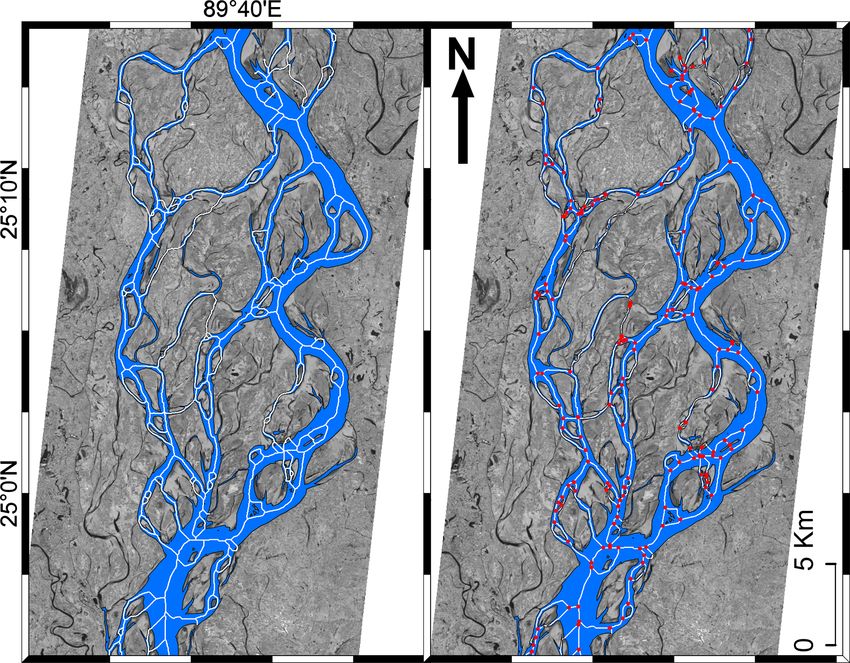
48                                                                                 K. Gaurav et al.: Coupling threshold theory

in the field (Leopold and Maddock, 1953). Equations that de-       established at 88 different gauging stations along six rivers in
fine the hydraulic geometry of a channel relate the width (W ),    the US and found that the exponents and coefficients are cor-
average depth (H ), and slope (S) of a channel to the bankfull     related. Recently, Kebede et al. (2020) used Landsat images
discharge (Q) according to                                         to estimate daily discharge of the Lhasa River in the Tibetan
                                                                   Plateau. They utilised image-derived hydraulic variables to
W = aQe ,                                                   (1)    compute the discharge using a modified Manning equation
         f                                                         and rating curves established from the in situ measurement
H = bQ ,                                                    (2)
S = cQ   −g
              ,                                             (3)    of width and discharge.
                                                                      The studies discussed above attempt to address the issue
where a, b, c, e, f , and g are site-specific constants and        of site-specificity, and they propose methods to estimate dis-
exponents. Therefore, the available methods (based on re-          charge without empirical calibration. However Bjerklie et al.
mote sensing data) to estimate the discharge of a river cannot     (2005), and Sun et al. (2010) also show that a better accu-
be extrapolated to other rivers or even to other locations on      racy in discharge prediction can only be achieved with some
the same river. Moreover, as these rating curves vary signif-      calibration to ground measurements. Therefore, a physically
icantly between locations, they must be established for each       robust method to resolve the site-specificity of rating curves
location independently. For example, Smith et al. (1995),          remains to be described.
Smith (1997), Smith and Pavelsky (2008), and Ashmore                  To address this issue of site-specificity, we have de-
and Sauks (2006) used synthetic aperture radar and ortho-          veloped a semi-empirical width–discharge regime relation
rectified aerial images to estimate discharge in braided rivers.   based on the threshold theory and field measurement of
They related the image-derived effective width of a braided        various braided and meandering rivers on the Ganga and
river to the discharge at a nearby gauging station to establish    Brahmaputra plains (Seizilles et al., 2013; Métivier et al.,
a relationship in the form of Eqs. (1)–(3). Their approach pro-    2016; Gaurav et al., 2017). According to this relation, threads
vides an estimate of the total discharge in a braided river, at    of braided and meandering rivers share a common width–
a given section. However, this technique is site-specific and      discharge regime relationship. Therefore, we hypothesise
assumes that the riverbed does not change over time.               that this regime equation can be used to estimate the first-
   Few attempts have been made to overcome these limi-             order discharge of any river (braided or meandering) flowing
tations; for example, Bjerklie et al. (2005) used aerial or-       on the Ganga and Brahmaputra plains (and perhaps on the
thophotographs and synthetic aperture radar (SAR) images           entire Himalayan foreland) if the wetted width of the river
to estimate discharge in various single-thread and braided         channels is known. This study can also be used for various
rivers. To estimate the discharge, they extracted the maxi-        applications such as (i) monitoring the downstream evolu-
mum water width at a given river reach. They then combined         tion of discharge, (ii) filling the data gap between the gauging
the image-derived channel widths with channel slopes ob-           stations separated over a long distance, (iii) constructing the
tained from topographic maps and a statistical hydrologic          time series and trend analysis of discharge variation, and (iv)
model. They reported standard errors of 50 %–100 %. How-           identifying the critical reaches in rivers that are under stress
ever, after using a calibration function based on field ob-        due to excessive extraction of water for agriculture, indus-
servation, the error decreased to values as low as 10 %.           trial, or domestic supply.
Later, Sun et al. (2010) used Japan Earth Resource Satellite-
1 (JERS-1) SAR images to measure the effective width of
the Mekong River at the Pakse gauging station in Laos. They        2   Hydrology of the Himalayan rivers
used a rainfall–runoff model to estimate the discharge from
the image-derived width and suggested that, using this pro-        Many rivers flowing on the Indus–Ganga–Brahmaputra al-
cedure, the discharge could be estimated in any ungauged           luvial plains are perennial and have their source in the Hi-
river basin within an acceptable level of accuracy. They es-       malayas and Tibetan Plateau. Flow of these rivers is primar-
tablished a close agreement between the measured discharge         ily determined by snowmelt and rainfall during the Indian
of the Mekong River at Pakse station and the model estimate        summer monsoon (Singh and Jain, 2002; Thayyen and Ger-
to the 90 % uncertainty level. As discussed earlier by Bjerklie    gan, 2010; Bookhagen and Burbank, 2010; Andermann et al.,
et al. (2005), Sun et al. (2010) subsequently indicated that the   2012; Khan et al., 2017). However, the contribution of rain-
precision can be improved by calibrating the rainfall–runoff       fall and snowmelt to the discharge of the Himalayan rivers
model with a hydraulic geometry relation and that a cali-          can vary significantly along the orogenic strike. For example,
brated rainfall–runoff model can be used to estimate the dis-      on an annual timescale, snowmelt contributes about 15 %–
charge in any ungauged river using the measured width only.        60 % of discharge in the western Himalayan rivers, whereas
Gleason and Smith (2014) have suggested that the discharge         it is less than 20 % in the eastern Himalayan rivers (Bookha-
of a single-thread river can be estimated from satellite im-       gen and Burbank, 2010). These rivers experience a strong
ages only, without any ground measurements. They plotted           seasonal variability in their discharge – for instance, rain-
the exponents and coefficients of hydraulic regime equations       fall during the Indian summer monsoon (June–September)

Earth Surf. Dynam., 9, 47–70, 2021                                                     https://doi.org/10.5194/esurf-9-47-2021
K. Gaurav et al.: Coupling threshold theory 49
constitutes about 60 %–85 % of the annual discharge of the Equation (4) is the theoretical equivalent to Lacey’s law.
eastern Himalayan catchments and about 50 % of the annual This theory explains the mechanism of how single-thread al-
discharge of the western Himalayan catchments. luvial rivers, at threshold of sediment transport, adjust their
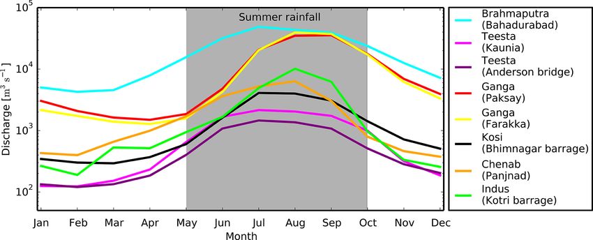
A closer look into the hydrographs of the Himalayan rivers geometry in response to the imposed water discharge. Strictly
reveals two distinct flow regimes (Fig. 1): a clear separation speaking, the mean equilibrium geometry of a natural allu-
of discharge during the summer monsoon and the rest of the vial channel is not set by a single discharge; rather, a range of
period can be observed. From May to October, most of the discharges are responsible for determining the channel form
Himalayan rivers flow at their peak discharge due to intense (Leopold and Maddock, 1953; Wolman and Miller, 1960;
and prolonged rainfall and glacier melt in the catchment; in Blom et al., 2017; Dunne and Jerolmack, 2020). However,
contrast, in the lean period (November–April), they carry rel- the value that corresponds to the channel-forming discharge
atively less discharge. of an alluvial river remains a matter of debate. Wolman and
Miller (1960); Wolman and Leopold (1957); Phillips and
3 Morphology of alluvial river Jerolmack (2016) proposed that the bankfull discharge and
discharge associated with a certain frequency distribution can
Lacey (1930) was the first to observe a dependency of the be used to define the channel-forming discharge.
width of an alluvial river on its discharge. Based on mea- As threshold theory predicts the scaling relationship of a
surements in various single-thread alluvial rivers and canals single-thread channel, one may consider applying it to assess
in India and Egypt, Lacey (1930) found that the width of the discharge that relates to the present-day geometry of nat-
a regime channel scales as the square root to the discharge ural alluvial channels. To test this, we use the regime curve
(e ∼ 0.5 in Eq. 1). that we established from threshold theory and the measure-
To explore the physical basis of the above-mentioned ob- ment of hydraulic geometry of various sandy alluvial rivers
servation, Glover and Florey (1951) and Henderson (1963) in the Himalayan foreland (Gaurav et al., 2014, 2017). In
developed a theory based on the concept of a threshold chan- field campaigns during 2012, 2013, 2014, and 2018, we mea-
nel. According to this theory, with a constant water dis- sured the geometry (width, depth, velocity, and median grain
charge, the balance between gravity and fluid friction main- size) of individual threads of braided and meandering rivers
tains the sediment at a threshold of motion, everywhere spanning the Ganga and Brahmaputra plains. To measure the
on the bed surface. This mechanism sets the cross-section channel geometry, we used an acoustic Doppler current pro-
shape and size of a channel. The resulting W –Qw (width– filer (ADCP) on an inflatable motor boat. Close to the loca-
discharge) relationship in dimensionless form reads as fol- tion of our ADCP-measured transects, we collected a sedi-
lows (Gaurav et al., 2014, 2017; Métivier et al., 2016, 2017): ment sample from the channel. We sieved the sediment sam-
" s # ple in the laboratory to calculate the median grain size (d50 ).
W π θt (ρs − ρf ) 0.25 3Cf Detailed descriptions of the measurement can be found in our
= Q0.5 ∗ , (4)
ds µ ρf 23/2 K 1/2 previous publications (Gaurav et al., 2014, 2017).
√ Figure 2 suggests that the individual threads of the Hi-
where Q∗ = Qw /(ds2 gds ) is the dimensionless water dis- malayan foreland rivers share a common width–discharge
charge, ds is the grain size, ρf ≈ 1000 kg m−3 is the den- regime relation, and their morphology can be explained by
sity of water, ρs ≈ 2650 kg m−3 is the density of quartz, threshold theory to the first order. The theoretical exponent
g ≈ 9.81 m s−2 is the acceleration of gravity, Cf ≈ 0.1 is accords with the empirical exponent of the width–discharge
the Chézy friction factor, µ ≈ 0.7 is the Coulomb coeffi- curve. However, the threads are wider than predicted by
cient of friction, K(1/2) ≈ 1.85 is the elliptic integral of the a factor of about 2 (Fig. 2). We now adjust the prefactor
first kind, and θt is the threshold Shields parameter that de- predicted from threshold theory to our data while retain-
pends on the sediments grain size. The typical grain size of ing the theoretical exponent to establish a generalised semi-
the sediments of the Himalayan foreland rivers is of the or- empirical “width–discharge” regime relationship for the Hi-
der of ds = 100–300 µm. Thus, the dimensionless grain size malayan foreland rivers (Fig. 2). We then use this curve to es-
D ∗ = (ds3 gρs2 /η2 )1/3 ' 1–6, where η ≈ 10−3 Pa s is the dy- timate the discharge of various rivers of the Himalayan fore-
namic viscosity of water. In this range of values, the thresh- land by measuring their width from satellite images.
old Shields number is on order of θt ∼ 0.1 with a maxi-
mum around 0.3 (Julien, 1995; Selim Yalin, 1992). Recently,
4 Material and methods
Delorme et al. (2017) obtained an experimental value of
θt ∼ 0.25 for silica sands with a size of 150 µm. Here, we 4.1 Dataset
have taken the upper value of θt = 0.3 as a conservative es-
timate. Taking lower values of the threshold Shields param- To measure the width of a river channel, we use images
eter, such as the classical 0.1, would lead to a slightly better acquired from Landsat Thematic Mapper (TM), Landsat
match between the theoretical prediction and the data, but it 8, and Sentinel-1A satellites (Appendix A1). All images
does not lead to a significant change in our conclusions. of the Landsat and Sentinel satellite missions are freely
https://doi.org/10.5194/esurf-9-47-2021 Earth Surf. Dynam., 9, 47–70, 2021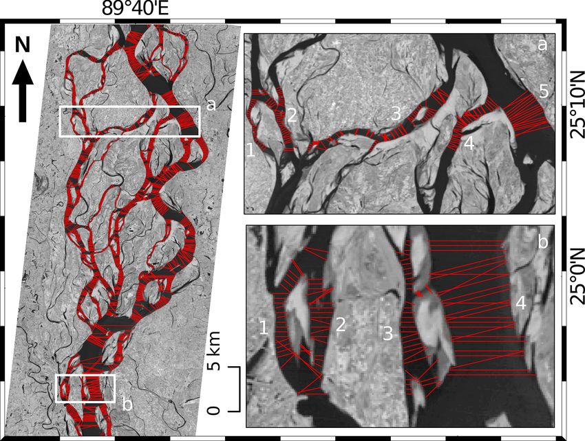
50                                                                                         K. Gaurav et al.: Coupling threshold theory

Figure 1. Hydrograph of the Himalayan rivers.

                                                                           an advanced synthetic aperture radar (ASAR) sensor that
                                                                           operates in the C-band (5.4 GHz) of microwave frequency
                                                                           (Schlaffer et al., 2015; Martinis et al., 2018). The advanced
                                                                           synthetic aperture radar system can operate both day and
                                                                           night and has the capability to penetrate clouds and heavy
                                                                           rainfall. This special characteristic of SAR sensors also en-
                                                                           ables uninterrupted imaging of the Earth’s surface during bad
                                                                           weather conditions.
                                                                              In situ measurements of average monthly discharge for
                                                                           time intervals of varying lengths between 1949 and 1975
                                                                           are available for the Brahmaputra, Teesta, Ganga, Chenab,
                                                                           and Indus rivers of the Himalayan foreland. They can be
                                                                           freely downloaded from http://www.rivdis.sr.unh.edu/maps
                                                                           (last access: July 2015). We obtained discharge data for
Figure 2. Dimensionless width of the individual threads of the Hi-         the 1996–2005 period for the Ganga River at Paksay sta-
malayan foreland rivers as a function of dimensionless water dis-          tion and the Brahmaputra River at Bahadurabad station from
charge (following Gaurav et al., 2017). These data (width, dis-            Bangladesh. Similarly, the Ganga River discharge from 1978
charge, and grain size) were acquired during the different field cam-      to 2007 measured at the Farakka station in India was obtained
paigns in the years 2012, 2013, 2014, and 2018. The measurements           from the Central Water Commission, Ministry of Water re-
were performed during the period when the Himalayan rivers usu-            sources, New Delhi. We also obtained discharge data for the
ally flow at their formative discharge. The solid line (dark) is the       Kosi River for the 2002–2014 period from the Investigation
prediction from threshold theory, and the solid line (light) is ob-        and Research Division, Kosi River Project, Birpur, and from
tained by fitting the prefactor of the threshold relation (Eq. 4) to the   our own field measurements (Appendix A2). We obtained the
data while retaining the theoretical exponent.
                                                                           median grain size of the bed sediments of the Kosi, Teesta,
                                                                           and Ganga rivers from our own field measurements, whereas
                                                                           measurements for the Chenab, Indus, and Brahmaputra rivers
available, and they can be downloaded from the US Ge-                      were obtained from the published literature (Goswami, 1985;
ological Survey (https://earthexplorer.usgs.gov, last access:              Dade and Friend, 1998; Gaurav et al., 2017; Khan et al.,
7 March 2019) and Alaska Satellite Facility (https://www.                  2019). The median grain size (d50 ) of our rivers varies in a
asf.alaska.edu/sentinel, last access: 7 March 2019) websites.              narrow range between 250 and 115 µm.
We downloaded all available cloud-free Landsat satellite im-
ages at the locations that were near the in situ measure-
                                                                           4.2   Width extraction
ment stations for which discharge data were available to us
(Fig. 3). Only a few cloud-free Landsat images are available               Our main objective is to extract the width of individual river
for the period from June to September. This is mainly be-                  channels from satellite images. We have developed an auto-
cause of the strong monsoon that causes intense rainfall and               mated program in Python 3.7 that takes a greyscale image
dense cloud cover. To overcome seasonal effect and fill the                as input to classify the image pixels into binary water and
data gap during the monsoon period, we use the Sentinel-1A                 non-water classes. The pixels classified as water are the fore-
product. The Sentinel-1 satellite mission is equipped with                 ground object and will be used to define river channels. Dry

Earth Surf. Dynam., 9, 47–70, 2021                                                             https://doi.org/10.5194/esurf-9-47-2021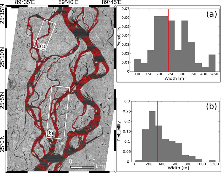
K. Gaurav et al.: Coupling threshold theory 51
Figure 3. Locations of the gauging stations of various rivers in the Indus, Ganga, and Brahmaputra basins for which discharge data are
available (source: © Google Earth).
pixels serve as a background object. To extract the river chan- pixels in size) that appear inside the river network do not cor-
nels, we use the infrared bands of Landsat TM and Landsat 8 respond to bars or islands. We found frequent areas where
images. In Landsat TM, the infrared (0.76–0.90 µm) wave- strong reflection from the bed sediment causes water pixels
length corresponds to band 4, whereas in Landsat 8, it cor- to appear more like sand. Isolated water pixels that do not be-
responds to band 5 (0.85–0.88 µm). The spatial resolution of long to the river are located in waterlogged areas. We identify
the infrared band for both Landsat (TM and 8) missions is these types of errors and reprocess the binary images to re-
30 m (pixel size: 30 m × 30 m). Theoretically, as water ab- move them automatically. Thus, we first identify the isolated
sorbs most of the infrared radiation, it appears dark, with an water patches from the binary images; to do this, we define
associated brightness value close to zero. This typical char- a 7 × 7 pixel search window. We run this window on the im-
acteristic of the infrared signal allows a clear distinction be- age and look for neighbouring water pixels in all surrounding
tween water-covered and dry areas on satellite images (Fra- directions. If a water pixel in the classified image is discon-
zier and Page, 2000). However, in the case of a river, the nected in all directions from the neighbouring water pixels
pixel intensity varies widely because of heterogeneous re- for more than seven pixels, we consider it to be an isolated
flectance of river water due to the presence of sediment and water body. Therefore, we reclassify such pixels as dry. We
organic particles (Nykanen et al., 1998). Because the image reiterate this procedure by applying a region-growing algo-
intensity is not exactly zero or one, we introduce a threshold rithm (Mehnert and Jackway, 1997; Bernander et al., 2013;
intensity to classify the pixels. Based on this criteria, we con- Fan et al., 2005). For this, we initially select a water seed
vert the greyscale image f (x, y) into a binary image g(x, y), pixel inside the river channel. The algorithm uses the initial
which distinguishes between the water-covered and dry ar- water pixels and starts growing. This procedure removes all
eas. This approach takes an object–background image and isolated water patches from the binary image and retains only
selects a threshold value that segments image pixels into ei- water pixels connected to the river network.
ther object (1) or background (0) (Ridler and Calvard, 1978; Once images are reclassified, we reprocess them to merge
Sezgin and Sankur, 2004). the water pixels that were initially classified as dry inside a
( river channel. For this, we define a 3 × 3 pixel search win-
0, if f (x, y) < T
g(x, y) = (5) dow. We choose this size by assuming that dry pixels should
1, if f (x, y) ≥ T be more than 90 m in size to be considered as bars or islands.
We apply the algorithm proposed by Yanni and Horne Otherwise, such pixels are treated as water pixels. We move
(1994) to obtain the threshold value iteratively. Once this op- the search window on the binary image and look for neigh-
timal value is obtained, we apply it to classify our pixels into bouring dry pixels inside the river channel.
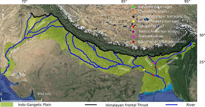
water and dry classes (Fig. 4). The binary classification of Similarly, to identify river pixels from Sentinel-1A im-
satellite images into water and dry pixels can also produce ages, we use the VH (vertical transmission and horizontal re-
spurious features (Fig. 4). ception) polarised band. The Sentinel Application Platform
These consist of wet pixels that get classified as dry or of (SNAP) v6.0 performs the radiometric calibration, speckle
isolated water pixels that appear randomly in the binary im- noise reduction using a refined Lee filter, and terrain cor-
ages (Passalacqua et al., 2013). Clusters (usually two–three rections, and finally generates the backscatter (σ0 ) image.
https://doi.org/10.5194/esurf-9-47-2021 Earth Surf. Dynam., 9, 47–70, 2021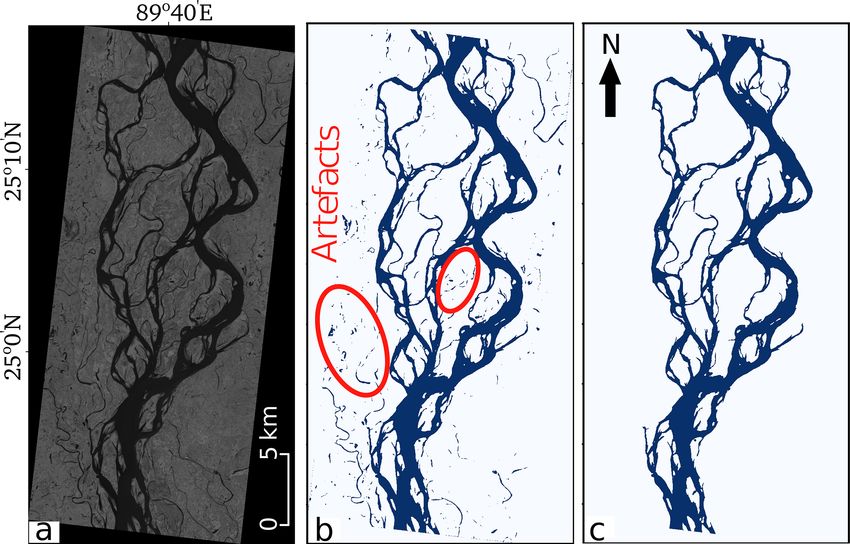
52                                                                                        K. Gaurav et al.: Coupling threshold theory

Figure 4. Histogram showing the distribution of pixel grey level intensity values. The optimal threshold (T ) value (marked with red line) is
obtained from the iterative threshold selection algorithm.

This image has a 60 m × 60 m pixel size that we resampled                are shallow and only a few pixels wide, their pixel intensity
at 30 m × 30 m to be consistent with the pixel size of Landsat           is close to the pixel intensity of dry areas. Therefore, the op-
images. In the microwave region, open and calm water bodies              timal threshold applied to categorise the image pixels does
exhibit low backscatter values due to high specular reflection           not identify these channels as water. Second, although an in-
from the water surface (Schlaffer et al., 2015; Twele et al.,            crease in the classification threshold could force the algo-
2016; Amitrano et al., 2018). We manually set a threshold                rithm to identify these pixels as water, it would also add sig-
value to separate water and dry pixels from Sentinel-1 im-               nificant noise by classifying many dry pixels as water pixels.
ages. Finally, we follow a similar procedure to the procedure            Such a limitation appears to be closely related to the image
that we developed for Landsat images to process the binary               resolution.
image obtained from Sentinel-1.                                             Given this qualitative agreement, we proceed to evaluate
   Once the satellite images are classified, we use the binary           the accuracy of the width extraction procedure. To do this,
images to extract the width of each channel. We do this by               we overlay the transects used by the algorithm to measure
measuring the distance from the centre of a channel to its               the width of a thread on the original image (Fig. 5a).
banks, orthogonal to the flow direction. A detailed automated               We then manually measure the width at randomly selected
procedure of the width extraction of a river channel is given            transects for comparison. For each river, we manually mea-
in Appendix B.                                                           sure the width at more than 15 randomly selected transects.
                                                                         We then compare the automatically extracted and manually
5     Result                                                             measured widths.
                                                                            Figure 6 compares the widths extracted automatically and
5.1    Accuracy assessment                                               manually. Most of the data points cluster on the 1 : 1 line.
                                                                         This indicates that, for the vast majority of threads, the width
To assess the precision with which we can estimate the dis-              computed from our automated procedure is almost equal to
charge of a thread, we need to quantify the accuracy of                  the width measured manually.
our width extraction procedure using Landsat and Sentinel-1                 However, there are some outliers. These outliers corre-
satellite images. To evaluate this, we superimpose the con-              spond to locations along the threads where our automated
tours of river channels, extracted using our algorithm, to the           procedure draws erroneous transects (Fig. 5b). Most of these
original greyscale images used for the extraction. We then               transects are located near highly curved reaches at the con-
carefully check for a match between the contours’ boundary               fluence or diffluence of two or more threads. In such places,
and water boundary in the greyscale image. We observed a                 the width of a thread is overestimated, sometimes by more
good agreement between the automatically extracted chan-                 than 50 %, compared with the manually measured width. At
nel boundary and the edge of the water line in the greyscale             most locations though, our procedure extracts valid transects
image. However, our algorithm fails to extract the contours              (Fig. 5a).
of the smallest channels (60–90 m in width). There are sev-
eral explanations for this limitation. First, as these channels

Earth Surf. Dynam., 9, 47–70, 2021                                                            https://doi.org/10.5194/esurf-9-47-2021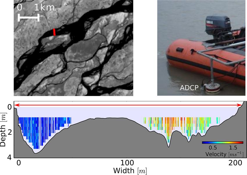
K. Gaurav et al.: Coupling threshold theory                                                                                               53

                                                                          Figure 7. Distribution of the error in the thread widths extracted
                                                                          automatically. The corresponding normal distribution is obtained by
                                                                          removing the 10 % extreme values from the distribution.

Figure 5. Width of the individual threads estimated across differ-
ent transects along a reach of the Brahmaputra River from Landsat         ages, particularly at locations where the curvature of a thread
satellite image. Panels (a) and (b) illustrate the regions of valid and   is high. The resulting skewness will be amplified in the dis-
erroneous transects at different places in the river (image source:       charge histogram because of the non-linear relationship re-
Landsat TM, 29 November 2013).                                            lating the two variables. To take the skewness into account,
                                                                          we have calculated the geometric mean of all of the measured
                                                                          values. The geometric mean is less affected by extreme val-
                                                                          ues in a skewed distribution and can be considered a repre-
                                                                          sentative width (Wr ). However, in meandering rivers where
                                                                          there is not much variability in width within a reach, the
                                                                          arithmetic mean can be considered a representative width.

                                                                          5.3   Discharge estimation
                                                                          We now proceed to estimate discharge (Qw ) for the Hi-
                                                                          malayan rivers based on their channel widths extracted from
                                                                          satellite images. To have a meaningful comparison between
                                                                          the image-derived discharge and the corresponding in situ
                                                                          measurement, we select a reach about 10 times longer than
Figure 6. Thread widths extracted using the automated technique           the width of a river on satellite images. In the case of a
are plotted as function of the manually extracted width.
                                                                          braided river, we consider the widest channel to define the
                                                                          reach length. In the selected reach, we assume that discharge
                                                                          is conserved: there is no significant addition or extraction of
   Furthermore, we assess the distribution of relative discrep-
                                                                          water in the river.
ancies between automatically and manually measured widths
                                                                             To estimate the discharge of the study reach, we use a
(Fig. 7). To quantify the precision of our measurements, we
                                                                          regime relation established by Gaurav et al. (2017) based on
compute the relative error. We observe that the relative er-
                                                                          threshold channel theory (Eq. 4) and field measurements of
ror of 90 % of our measurements is centred around a mean
                                                                          a channel’s width and discharge on the Ganga–Brahmaputra
µ ≈ −0.02 with a standard deviation σ ≈ 0.07. This vali-
                                                                          plains. The resulting regime relation is governed by
dates the width extraction procedure.
                                                                                   2
                                                                                    Wr p
                                                                          Qw =              (gds ),                                   (6)
5.2   Width variability along a thread                                               α
Particularly in a braided river, the width of a thread varies sig-        where α is the best-fit coefficient, an empirical value obtained
nificantly along its course. To quantify this variability, we se-         from fitting the prefactor of the regime curve (Eq. 4), Wr is
lect a reach and plot the probability distribution of the width           the representative width, and ds is the median grain size.
measured across different transects. We observed that the dis-               We use Eq. (6) to calculate the discharge for threads of
tribution of width histograms is skewed (Fig. 8). This skew-              known width. Because the river width scales non-linearly
ness results from the natural variability in width along the              with discharge, the regime relations obtained refer to the to-
course and also due to the error in width extraction from im-             tal width in the case of a braided river, and they will not be

https://doi.org/10.5194/esurf-9-47-2021                                                            Earth Surf. Dynam., 9, 47–70, 2021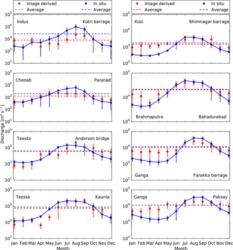
54                                                                                        K. Gaurav et al.: Coupling threshold theory

Figure 8. Spatial distribution of the width measured along the threads of a braided reach of the Ganga River near the Paksay gauging station
in Bangladesh. The vertical line (red) on the histograms in panels (a) and (b) represents the geometric mean that corresponds to the most
probable width (Wm ).

the same as those obtained for individual threads. As most              compares the estimated and measured discharges during the
of the studied rivers are braided, we first calculate the dis-          monsoon period. For most of our rivers, the difference be-
charge for individual threads across a given section. We then           tween measured and estimated discharges is less than 50 %,
sum the discharge of the individual threads across a transect           although this difference is comparatively high for the Indus
to compute the total discharge at a section.                            (72 %–78 %) and Chenab (36 %–67 %) rivers (Table 2).

5.4   Estimated vs. measured discharge
                                                                        6   Discussion
Once monthly discharges for all of the rivers are estimated
from satellite images, we compare them with the average                 It is important to note that the discharge estimated from
monthly discharge measured at the corresponding gauging                 satellite images does not correspond to an instantaneous dis-
stations. To do so, we plot the hydrographs of the estimated            charge. To understand the emergence of a constant hydro-
and measured discharges together (Fig. 9). We observed that             graph from the estimated discharge derived from satellite im-
the estimated discharge of the Kosi, Ganga, and Brahmaputra             ages, we explore the concept of channel-forming (formative)
rivers from satellite images is overestimated and almost con-           discharge, i.e. a discharge that sets the geometry of alluvial
stant throughout during the non-monsoon period (October–                river channels. Several workers, including Inglis and Lacey
May). Conversely, the Indus, Chenab, and Teesta rivers show             (1947), Leopold and Maddock (1953), and Blench (1957),
a clear annual cycle. This observed trend is not entirely clear         have shown that the geometry of an alluvial channel corre-
to us, but it could possibly be related to the flow regulation,         sponds to a formative discharge (see Table A3 in the Ap-
as these river are highly regulated through a series of dams            pendix for the definition of different discharges). They have
and barrages.                                                           discussed how a limited range of flows are responsible for
   Furthermore, we observed that the estimated discharge for            shaping its channel. At low-flow discharge, the water sim-
most of our rivers show a significant rise during the mon-              ply flows through the threads without affecting their geom-
soon period (June–September). To the first order, it appears            etry. Schumm and Lichty (1965) used the concept of time
that our approach is able to capture the rising trend of dis-           span (geologic, modern, and present) in defining the inter-
charges during the monsoon period; however, the estimated               relationship between dependent and independent variables
discharges are lesser than the measured discharges. Table 2             of a river system. According to these authors, the morphol-

Earth Surf. Dynam., 9, 47–70, 2021                                                            https://doi.org/10.5194/esurf-9-47-2021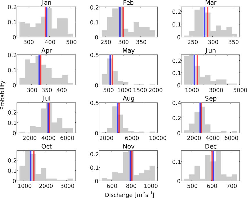
K. Gaurav et al.: Coupling threshold theory                                                                                                55

Figure 9. Hydrograph of satellite-derived reach-averaged discharge against their monthly average discharge recorded at the gauging station.
The error bar in the measured discharge (blue) is the standard deviation calculated from the time series of different months; the error bar in
the estimated discharge represents the standard deviation within the study reach. Dotted red and blue lines are the annual average discharge
obtained from satellite images and in situ measurement respectively.

ogy of a river channel is set in the modern time span (last              the discharge hydrographs estimated from the measurement
1000 years) by the average discharge of water and sediment.              of channels’ width from the satellite images (Fig. 9). Fur-
In the present time span (1 year or less), channel morphology            thermore, Métivier et al. (2017) have recently shown that
can be considered as an independent variable against instan-             non-cohesive streams laden with sediments cannot have a
taneous discharge of water and sediment.                                 width much larger than the width of a threshold stream before
   Similarly, it has been argued by Inglis and Lacey (1947),             they start to braid. They also showed that, for experimental
Leopold and Maddock (1953), and Blench (1957) that it is                 braided rivers, threads are always formed at the bankfull flow
not the highest flows that contribute the most in shaping a              and at the limit of stability. Thus, our hypothesis is that the
river channel. Such high discharges are capable of transform-            formative discharge of threads in the Ganga plain is the bank-
ing the channel, but they occur so infrequently that, on aver-           full discharge. This is probably why our estimated discharge
age, their morphological impact is small. Wolman and Miller              from satellite images remain constant throughout the non-
(1960) highlighted that the bankfull discharge that occurs               monsoon period for most of the rivers and is mostly over-
once each year or every 2 years sets the pattern and chan-               estimated compared with the measured discharge at gauging
nel width of the alluvial rivers. Formative discharge for the            stations.
Himalayan rivers is expected to occur in the monsoon pe-                    According to Inglis and Lacey (1947), rivers approach
riod; thus, during low flow, one may expect that such rivers             their equilibrium geometry for a formative discharge that
maintain their flows without modifying the existing channel              approximately corresponds to the bankfull discharge. They
geometry (Roy and Sinha, 2014). This is clearly reflected in             suggested this discharge lies between half and two-thirds

https://doi.org/10.5194/esurf-9-47-2021                                                            Earth Surf. Dynam., 9, 47–70, 2021
56                                                                                       K. Gaurav et al.: Coupling threshold theory

Table 1. Comparison between the image-derived discharge and the discharge measured in situ for the Himalayan rivers during the Indian
summer monsoon period. The error in the measured discharge is the standard deviation calculated from the time series of different months;
the error in the estimated discharge is the standard deviation within the study reach.

                                                                              Monsoon discharge [m3 s−1 ]
       Rivers                                                       June                July               August        September
       Kosi (Bhimnagar barrage)         In situ              1616 ± 285         4091 ± 530          3998 ± 660          3072 ± 509
                                        Image derived        1515 ± 797         2800 ± 912         3660 ± 1667         2796 ± 1644
                                        Difference (%)              −6                −32                  −8                  −9
       Brahmaputra (Bahadurabad)        In situ           31 717 ± 5536      48 769 ± 9640        43 387 ± 8722       39 320 ± 8071
                                        Image derived    35 335 ± 10 491    39 716 ± 15 914       40 653 ± 9808      37 316 ± 12 580
                                        Difference (%)                11               −19                  −6                   −5
       Ganga (Farakka barrage)          In situ             4260 ± 2989      20 375 ± 6059       39 462 ± 10 665      37 264 ± 9415
                                        Image derived       6864 ± 3717      20 599 ± 9343        24 562 ± 8871       18 971 ± 7364
                                        Difference (%)               61                  1                  −38                −49
       Ganga (Paksay)                   In situ            4794 ± 3425       20 691 ± 5427        34 887 ± 9002       35 546 ± 8985
                                        Image derived     10 226 ± 4689      15 333 ± 6510        18 862 ± 7691       19 168 ± 8089
                                        Difference                  113               −26                  −46                 −46
       Teesta (Anderson bridge)         In situ              1078 ± 204         1458 ± 330           1363 ± 395          1076 ± 416
                                        Image derived         356 ± 139          904 ± 494           2086 ± 494          1079 ± 759
                                        Difference (%)             −67                −38                    53                   0
       Teesta (Kaunia)                  In situ              1674 ± 428         2151 ± 792          2037 ± 369           1733 ± 227
                                        Image derived         860 ± 700         1765 ± 883         1938 ± 1036           2346 ± 540
                                        Difference (%)             −49                −18                  −5                    35
       Indus (Kotri barrage)            In situ             1665 ± 1136       4912 ± 3290         10 128 ± 5807        6227 ± 3980
                                        Image derived         372 ± 238         861 ± 417          2279 ± 1279          1759 ± 826
                                        Difference (%)             −78               −82                   −77                −72
       Chenab (Panjnad)                 In situ             3621 ± 2812       5235 ± 3206          6340 ± 2983         3038 ± 1574
                                        Image derived       2300 ± 1302        2125 ± 988          2099 ± 1193          1311 ± 749
                                        Difference (%)             −36               −59                  −67                 −57

Table 2. Comparison between the annual average discharge measured at the gauging stations and that estimated from satellite images.

                          River            Station             hQinsitu i          hQsat. i      Qdiff.     Qdiff.
                                                               [m3 s−1 ]         [m3 s−1 ]     [m3 s−1 ]     [%]
                          Teesta           Anderson           605 ± 109         638 ± 165           33          5
                          Teesta           Kaunia             924 ± 144         745 ± 155         −179         19
                          Kosi             Bhimnagar         1559 ± 313        1810 ± 380          251         16
                          Chenab           Panjnad           2500 ± 961        1275 ± 268        −1225         49
                          Indus            Kotri             3745 ± 825         794 ± 162        −2951         78
                          Ganga            Farakka        11 477 ± 2279     10 593 ± 2225         −884          8
                          Ganga            Paksay         12 080 ± 2403     11 605 ± 2438         −475          4
                          Brahmaputra      Bahadurabad    21 751 ± 2942     21 717 ± 4740          −34
K. Gaurav et al.: Coupling threshold theory 57
charges on a log–log scale (Fig. 10). The discharge estimated
from satellite images agrees to within an order of magnitude
with the measured discharge.
The differences between the measured and estimated an-
nual average discharges for the Brahmaputra, Ganga, Kosi,
and Teesta rivers are less than 20 %. However, this differ-
ence is comparatively high for the Indus (78 %) and Chenab
(49 %) rivers. Interestingly, the estimated discharges for the
Teesta (at Anderson station), Ganga (at Farakka and Pak-
say), and Brahmaputra (at Bahadurabad) rivers converge to
their measured discharges with small differences of 5 %, 8 %,
4 %, and < 1 % respectively (Table 2); in contrast, the esti-
mated discharges of the Teesta (at Kaunia station) and Kosi
(at Bhimnagar) show a relatively higher differences of 19 %
and 16 % respectively. These differences could possibly be
related to the anthropogenic impact on the natural flow con-
Figure 10. Satellite-derived river discharge against annual average
dition. For example, the selected study reaches for the Teesta
discharge measured at a ground station. The error bar in the mea-
sured discharge represents the standard deviation; the error bar for (at Kaunia station) and Kosi (at Bhimnagar) rivers are lo-
the estimated discharge is calculated by considering ±10 % mea- cated near the barrage where flow is regulated. However, this
surement uncertainty in the channel widths from satellite images. relationship is not entirely clear at this stage.
Similarly, the observed annual cycle in discharge and the
large difference between the estimated and measured dis-
charge of the Indus and Chenab rivers could possibly be re-
complex topography of the bed. As an example, Fig. C1 in lated to a series of dams and barrages (Kotri barrage, 1955;
the Appendix, illustrates the cross section of a braided thread Mangla dam, 1967; Tarbela dam, 1976) that have been con-
measured in the field using an acoustic Doppler current pro- structed. Such anthropogenic intervention has significantly
filer (ADCP). This high-resolution bathymetric profile en- altered the water and sediment discharge of the Indus River.
ables us to identify the two different threads separated by For example, downstream of the Kotri barrage, the average
submerged bars and islands. In such situations, discharge is annual water discharge of the Indus River has declined at an
not carried across the width seen from the plan view but only alarming rate from about 107 × 109 m3 to 10 × 109 m3 from
through the narrow active regions. Furthermore, this indi- 1954 to 2003 (Inam et al., 2007). This continuous decline in
cates that during low flow, water spread in the existing geom- the average annual discharge might have significantly modi-
etry is set at the formative discharge. Currently, satellite im- fied the geometry of the Indus River.
ages allow us to measure the top width of the water surface. Furthermore, to understand our estimates of discharge for
For a given thread, we presume that discharge estimated from the Chenab, Indus, and Teesta rivers, we plot their monthly
these widths should compare to the formative discharge. discharge time series recorded at the corresponding gauging
We now evaluate how the discharge estimated from satel- stations against the discharge estimated from satellite images
lite data varies with time. We plot the monthly discharge es- (Figs. C3 and C4 in the Appendix). Despite a large vari-
timated for all of our rivers to their corresponding average ability, the discharge time series of the Indus and Chenab
monthly discharge measured at the gauging stations (Fig. 9 rivers show a strong declining trend during the monsoon pe-
in the Appendix). The monthly average discharge of the Hi- riod (June–September), whereas discharge during the non-
malayan foreland rivers appears to be a representative of monsoon period appears to remain constant around the mean
the actual hydrograph (Fig. C2). As suggested earlier by In- value. Figure C3 in the Appendix clearly shows that dis-
glis and Lacey (1947), Leopold and Maddock (1953), and charge estimated from satellite images plots within the vari-
Blench (1957), we observe that except for the Indus, Chenab, ability of the observed trend. The estimated discharge of the
and Teesta rivers, the estimated discharges from images are Teesta River also plots within the noise of the observed trend.
nearly constant throughout during the non-monsoon period, This gives us confidence in our estimates of discharge, espe-
with small fluctuations around their mean. This supports the cially for the rivers for which we have a limited, old record
hypothesis that the width of the thread extracted from satel- (1973–1979) of in situ discharges.
lite images corresponds to a value closer to the formative dis- In a recent study, Allen and Pavelsky (2018) measured
charge. the width of the global rivers from Landsat images for the
To extend upon this, we now compare the annual average month when they commonly flow near mean discharge. We
discharge estimated from Landsat and Sentinel-1A images have used the water mask binary images from the Global
for different months to the annual average discharge mea- River Width from Landsat (GRWL) database and measured
sured at corresponding ground stations. We plot these dis- the thread widths of the Brahmaputra, Chenab, Ganga, Indus,
https://doi.org/10.5194/esurf-9-47-2021 Earth Surf. Dynam., 9, 47–70, 202158 K. Gaurav et al.: Coupling threshold theory
and Teesta rivers (Appendix C). We used these widths to es- we have estimated the discharge of six major rivers in the
timate discharges using our regime curve and compare them Himalayan foreland (Brahmaputra, Chenab, Ganga, Indus,
with the mean annual discharge recorded at the correspond- Kosi, and Teesta). Our estimated discharges closely com-
ing gauging station as well as our estimates from satellite im- pare with the average annual discharge measured at the near-
ages. For most of our rivers, we observed that the discharge est gauging stations. This first-order agreement, although en-
estimated from the thread’s width extracted from the GRWL couraging, requires further research to improve the degree of
database of Allen and Pavelsky (2018) falls within the same agreement between measured and estimated discharges. One
order of magnitude as the yearly average discharge measured of the main sources of uncertainty in the discharge estimate is
at the corresponding gauging stations (Table C1). For most due to the error in the measurement of thread widths. This de-
rivers, the difference between the measured and estimated pends on the image resolution and accuracy of the algorithm
discharge from GRWL data is approximately less than 60 %. used for the extraction of river pixels from remotely sensed
However, this difference is comparatively high for the Kosi images. Better-resolution remote sensing images would most
(88 %) and Indus (95 %) rivers. Interestingly, in accordance likely minimise the uncertainty and improve the agreement
to our estimates, the GRWL database also shows a high re- between estimated and in situ discharge. Furthermore, our
duction in the discharge of the Indus and Chenab rivers from regime equation established for the Himalayan rivers is based
the measured discharge at their corresponding ground sta- on a simple physical mechanism that explains the geometry
tions during the period from 1973 to 1979. of alluvial channels. Therefore, we suspect that the procedure
The GRWL database is a first ever compilation of width we have established could be extended to most alluvial rivers.
for the global rivers, and it may be used together with our Globally, it has been observed that the threshold theory well
regime curve to obtain a first-order approximation of the for- predicts the exponent of the regime equation (Eq. 6); how-
mative discharge of the Himalayan foreland rivers. ever, the prefactor may vary significantly depending on the
grain size distribution, the turbulent friction coefficient, and
the critical Shields parameter (Métivier et al., 2017). It is,
7 Conclusions and future outlook therefore, suggested that this regime curve is modified using
measurements of the width, discharge, and grain size of indi-
The semi-empirical regime relation established by Gaurav vidual threads of alluvial channels in the field before apply-
et al. (2017) and remote sensing images can be used to ob- ing it to rivers with different climatic regimes. Moreover, it
tain a first-order estimate of the formative discharge of the should be noted that our regime curve relates to the measure-
rivers of the Himalayan foreland, if their channel width is ment of hydraulic geometry of individual threads of braided
known. The regime equation used here is established from and meandering rivers; therefore, it is applicable only at the
the recent measurements and the published data by Gaurav thread scale. As the resulting regime curve is non-linear, es-
et al. (2014, 2017). This equation is based on threshold the- timating discharge across a transect in a braided river from
ory and instantaneous measurements of the hydraulic geom- the aggregated width will be different from the discharge ob-
etry of individual threads of various braided and meandering tained after the summation of discharges of the individual
rivers. The measurements were acquired during the period threads.
when rivers of the Himalayan foreland usually flow at their This study presents a robust methodology and is a step to-
formative discharge (Roy and Sinha, 2014). Therefore, this wards obtaining first-order estimates of formative discharge
regime equation only provides an estimate of the formative in ungauged river basins solely from remote sensing images.
discharge, and it can not capture the instantaneous variations It can be used for sustainable river development and man-
in discharge. On the other hand, as this regime relation is agement to ensure regional water security and flood manage-
established from the measurements in braided and meander- ment, especially in regions where river discharge data are not
ing rivers, it can be used to establish first-order estimates of readily available.
formative discharge in a river of any planform. It is espe-
cially useful and relevant for braided rivers that present sev-
eral difficulties with respect to the measurement of discharge
in the field. Our regime equation requires only one parameter
(grain size) to estimate discharge from width measurements.
It can be obtained easily from field measurements. As our
regime equation is established from measurements of a wide
range of channels spanning over the Ganga and Brahmaputra
plains, we believe that it can be used to obtain a first-order es-
timate of the formative discharge of rivers in the Himalayan
foreland by just measuring their channel width on satellite
or aerial images. Using our semi-empirical regime equation
and satellite images of the Landsat and Sentinel-1 missions,
Earth Surf. Dynam., 9, 47–70, 2021 https://doi.org/10.5194/esurf-9-47-2021K. Gaurav et al.: Coupling threshold theory 59
Appendix A: Dataset
A1 Satellite images
In this section, a detailed specification of the satellite data
(Landsat and Sentinel-1) used in this study is given.
Table A1. Details of the Landsat 8 (L-8), Landsat TM (L-TM), and Sentinel-1A (S-1A) satellite images used in this study. “Gauging station”
is the location (◦ N, ◦ E) of the nearest in situ discharge measurement station.
Landsat TM and Landsat 8
River Date (yyyy/mm/dd) Scene ID Satellite Gauging station
Brahmaputra 2009-01-18 LT51380432009018KHC01 L-TM 25.18, 89.66
Brahmaputra 2009-02-19 LT51380432009050KHC00 L-TM 25.18, 89.66
Brahmaputra 2014-03-21 LC81380432014080LGN00 L-8 25.18, 89.66
Brahmaputra 2014-04-22 LC81380432014112LGN00 L-8 25.18, 89.66
Brahmaputra 2014-10-31 LC81380432014304LGN00 L-8 25.18, 89.66
Brahmaputra 2013-11-29 LC81380432013333LGN00 L-8 25.18, 89.66
Brahmaputra 2014-12-02 LC81380432014336LGN00 L-8 25.18, 89.66
Chenab 2014-01-04 LC81500402014004LGN00 L-8 29.35, 71.30
Chenab 2018-02-16 LC81500402018047LGN00 L-8 29.35, 71.30
Chenab 2015-04-13 LC81500402015103LGN00 L-8 29.35, 71.30
Chenab 2014-05-28 LC81500402014148LGN00 L-8 29.35, 71.30
Chenab 2014-06-29 LC81500402014180LGN00 L-8 29.35, 71.30
Chenab 2014-07-15 LC81500402014196LGN00 L-8 29.35, 71.30
Chenab 2014-10-19 LC81500402014292LGN00 L-8 29.35, 71.30
Chenab 2013-11-01 LC81500402013305LGN00 L-8 29.35, 71.30
Chenab 2014-12-06 LC81500402014340LGN00 L-8 29.35, 71.30
Ganga 2015-02-11 LC81390432015042LGN01 L-8 24.83, 87.92
Ganga 2015-03-15 LC81390432015074LGN00 L-8 24.83, 87.92
Ganga 2013-04-02 LT51390432010092KHC00 L-8 24.83, 87.92
Ganga 2014-06-16 LC81390432014167LGN00 L-8 24.83, 87.92
Ganga 2014-11-23 LC81390432014327LGN00 L-8 24.83, 87.92
Ganga 2009-01-18 LT51380432009018KHC01 L-TM 24.08, 89.03
Ganga 2009-02-19 LT51380432009050KHC00 L-TM 24.08, 89.03
Ganga 2014-03-21 LC81380432014080LGN00 L-8 24.08, 89.03
Ganga 2014-04-22 LC81380432014112LGN00 L-8 24.08, 89.03
Ganga 2014-10-31 LC81380432014304LGN00 L-8 24.08, 89.03
Ganga 2013-11-29 LC81380432013333LGN00 L-8 24.08, 89.03
Ganga 2014-12-02 LC81380432014336LGN00 L-8 24.08, 89.03
Indus 2015-01-05 LC81520422015005LGN00 L-8 25.35, 68.35
Indus 2017-02-11 LC81520422017042LGN00 L-8 25.35, 68.35
Indus 2015-03-10 LC81520422015069LGN00 L-8 25.35, 68.35
Indus 2014-04-24 LC81520422014114LGN00 L-8 25.35, 68.35
Indus 2014-06-27 LC81520422014178LGN00 L-8 25.35, 68.35
Indus 2014-10-17 LC81520422014290LGN00 L-8 25.35, 68.35
Indus 2014-11-18 LC81520422014162LGN00 L-8 25.35, 68.35
Kosi 1991-01-15 LT51400421991015ISP00 L-TM 26.52, 86.92
Kosi 2011-02-07 LT51400422011038BKT00 L-TM 26.52, 86.92
Kosi 1992-03-06 LT51400421992066ISP00 L-TM 26.52, 86.92
Kosi 2018-05-01 LC81400422018121LGN00 L-8 26.52, 86.92
Kosi 2015-09-30 LC81400422015273LGN01 L-8 26.52, 86.92
Kosi 2000-10-14 LE71400422000288SGS00 L-TM 26.52, 86.92
Kosi 2013-11-11 LC81400422013315LGN00 L-TM 26.52, 86.92
Kosi 2002-12-07 LE71400422002341SGS00 L-TM 26.52, 86.92
https://doi.org/10.5194/esurf-9-47-2021 Earth Surf. Dynam., 9, 47–70, 202160 K. Gaurav et al.: Coupling threshold theory
Table A1. Continued.
Landsat TM and Landsat 8
River Date (yyyy/mm/dd) Scene ID Satellite Gauging station
Teesta 2014-04-22 LC81380422014112LGN00 L-8 26.33, 88.87
Teesta 2014-10-31 LC81380422014304LGN00 L-8 26.33, 88.87
Teesta 2014-11-16 LC81380422014320LGN00 L-8 26.33, 88.87
Teesta 2014-12-02 LC81380422014336LGN00 L-8 26.33, 88.87
Teesta 2015-03-08 LC81380422015067LGN00 L-8 25.70, 89.50
Teesta 2014-04-22 LC81380422014112LGN00 L-8 25.70, 89.50
Teesta 2014-10-31 LC81380422014304LGN00 L-8 25.70, 89.50
Teesta 2014-12-02 LC81380422014336LGN00 L-8 25.70, 89.50
Sentinel-1A
Ganga 2017-10-17 S1A_IW_GRDH · · · _31A9_Cal_Spk_TC S-1A 24.83, 87.92
Ganga 2018-07-20 S1A_IW_GRDH · · · _BE68_Cal_Spk_TC S-1A 24.83, 87.92
Ganga 2018-05-18 S1A_IW_GRDH · · · _114F_Cal_Spk_TC S-1A 24.83, 87.92
Ganga 2018-08-10 S1A_IW_GRDH · · · _6C38_Cal_Spk_TC S-1A 24.83, 87.92
Ganga 2018-09-06 S1A_IW_GRDH · · · _4CBB_Cal_Spk_TC S-1A 24.83, 87.92
Ganga 2016-04-13 S1A_IW_GRDH · · · _4BF4_Cal_Spk_TC S-1A 24.83, 87.92
Ganga 2018-01-18 S1A_IW_GRDH · · · _831D_Cal_Spk_TC S-1A 24.83, 87.92
Ganga 2017-09-27 S1A_IW_GRDH · · · _2DC4_Cal_Spk_TC S-1A 24.08, 89.03
Ganga 2018-05-13 S1A_IW_GRDH · · · _EF71_Cal_Spk_TC S-1A 24.08, 89.03
Ganga 2018-06-08 S1A_IW_GRDH · · · _035D_Cal_Spk_TC S-1A 24.08, 89.03
Ganga 2018-07-12 S1A_IW_GRDH · · · _8CBA_Cal_Spk_TC S-1A 24.08, 89.03
Ganga 2018-08-17 S1A_IW_GRDH · · · _EF93_Cal_Spk_TC S-1A 24.08, 89.03
Brahamputra 2018-07-14 S1A_IW_GRDH · · · _2752_Cal_Spk_TC S-1A 25.18, 89.66
Brahamputra 2017-11-14 S1A_IW_GRDH · · · _BA85_TC_Cal S-1A 25.18, 89.66
Brahamputra 2018-05-15 S1A_IW_GRDH · · · _9533_Cal_Spk_TC S-1A 25.18, 89.66
Brahamputra 2017-09-17 S1A_IW_GRDH · · · _E022_Cal_Spk_TC S-1A 25.18, 89.66
Brahamputra 2018-06-18 S1A_IW_GRDH · · · _8D0F_Cal_Spk_TC S-1A 25.18, 89.66
Brahamputra 2018-08-19 S1A_IW_GRDH · · · _173D_Cal_Spk_TC S-1A 25.18, 89.66
Chenab 2018-09-07 S1A_IW_GRDH · · · _3240_Cal_Spk_TC S-1A 29.35, 71.30
Chenab 2018-08-14 S1A_IW_GRDH · · · _A3CB_Cal_Spk_TC S-1A 29.35, 71.30
Chenab 2018-03-19 S1A_IW_GRDH · · · _2E5E_Spk_TC S-1A 29.35, 71.30
Chenab 2018-02-23 S1A_IW_GRDH · · · _741E_TC_Cal_Spk S-1A 29.35, 71.30
Indus 2018-07-10 S1A_IW_GRDH · · · _4B89_Cal_Spk_TC S-1A 25.35, 68.35
Indus 2018-05-11 S1A_IW_GRDH · · · _CE83_Cal_Spk_TC S-1A 25.35, 68.35
Indus 2017-09-13 S1A_IW_GRDH · · · _7DD5_Cal_Spk_TC S-1A 25.35, 68.35
Indus 2018-08-27 S1A_IW_GRDH · · · _DA34_Cal_Spk_TC S-1A 25.35, 68.35
Teesta 2017-09-03 S1A_IW_GRDH · · · _32D8_Cal_Spk_T S-1A 25.70, 89.50
Teesta 2018-01-13 S1A_IW_GRDH · · · _022569 S-1A 25.70, 89.50
Teesta 2018-05-13 S1A_IW_GRDH · · · _021886 S-1A 25.70, 89.50
Teesta 2018-06-06 S1A_IW_GRDH · · · _022236 S-1A 25.70, 89.50
Teesta 2018-07-12 S1A_IW_GRDH · · · _022761 S-1A 25.70, 89.50
Teesta 2018-08-29 S1A_IW_GRDH · · · _023461 S-1A 25.70, 89.50
Teesta 2017-09-03 S1A_IW_GRDH · · · _32D8_Cal_Spk_TC S-1A 26.33, 88.87
Teesta 2018-01-13 S1A_IW_GRDH · · · _50B1_Cal_Spk_TC S-1A 26.33, 88.87
Teesta 2018-05-13 S1A_IW_GRDH · · · _D8D7_Cal_Spk_TC S-1A 26.33, 88.87
Teesta 2018-06-06 S1A_IW_GRDH · · · _1753_Cal_Cal_TC S-1A 26.33, 88.87
Teesta 2018-07-12 S1A_IW_GRDH · · · _F499_Cal_Spk_TC S-1A 26.33, 88.87
Teesta 2018-08-29 S1A_IW_GRDH · · · _341E_Cal_Spk_TC S-1A 26.33, 88.87
Kosi 2018-08-18 S1A_IW_GRDH · · · _8CB2_Cal_Spk_TC S-1A 26.52, 86.92
Kosi 2018-06-19 S1A_IW_GRDH · · · _9B41_Cal_Spk_TC S-1A 26.52, 86.92
Kosi 2017-04-25 S1A_IW_GRDH · · · _32C5_Cal_Spk_TC S-1A 26.52, 86.92
Kosi 2017-07-30 S1A_IW_GRDH · · · _2658_Cal_Spk_TC S-1A 26.52, 86.92
Earth Surf. Dynam., 9, 47–70, 2021 https://doi.org/10.5194/esurf-9-47-2021You can also read