COVID-19 lockdown-induced changes in NO2 levels across India observed by multi-satellite and surface observations - Recent
←
→
Page content transcription
If your browser does not render page correctly, please read the page content below
Atmos. Chem. Phys., 21, 5235–5251, 2021
https://doi.org/10.5194/acp-21-5235-2021
© Author(s) 2021. This work is distributed under
the Creative Commons Attribution 4.0 License.

COVID-19 lockdown-induced changes in NO2 levels across India
observed by multi-satellite and surface observations
Akash Biswal1,2 , Vikas Singh1 , Shweta Singh1 , Amit P. Kesarkar1 , Khaiwal Ravindra3 , Ranjeet S. Sokhi4 ,
Martyn P. Chipperfield5,6 , Sandip S. Dhomse5,6 , Richard J. Pope5,6 , Tanbir Singh2 , and Suman Mor2
1 National Atmospheric Research Laboratory, Gadanki, AP, India
2 Department  of Environment Studies, Panjab University, Chandigarh 160014, India
3 Department of Community Medicine and School of Public Health, Post Graduate Institute of Medical Education and

Research (PGIMER), Chandigarh 160012, India
4 Centre for Atmospheric and Climate Physics Research (CACP), University of Hertfordshire, Hatfield, UK
5 School of Earth and Environment, University of Leeds, Leeds, UK
6 National Centre for Earth Observation, University of Leeds, Leeds, UK

Correspondence: Vikas Singh (vikas@narl.gov.in)

Received: 1 October 2020 – Discussion started: 13 October 2020
Revised: 9 February 2021 – Accepted: 2 March 2021 – Published: 1 April 2021

Abstract. We have estimated the spatial changes in NO2 lev-        urban areas as the decrease at the surface was masked by en-
els over different regions of India during the COVID-19 lock-      hancement in NO2 due to the transport of the fire emissions.
down (25 March–3 May 2020) using the satellite-based tro-
pospheric column NO2 observed by the Ozone Monitoring
Instrument (OMI) and the Tropospheric Monitoring Instru-
ment (TROPOMI), as well as surface NO2 concentrations              1   Introduction
obtained from the Central Pollution Control Board (CPCB)
monitoring network. A substantial reduction in NO2 levels          Nitrogen oxides, NOx (NO + NO2 ), are one of the major
was observed across India during the lockdown compared             air pollutants, as defined by various national environmen-
to the same period during previous business-as-usual years,        tal agencies across the world, due to their adverse impact
except for some regions that were influenced by anomalous          on human health (Mills et al., 2015). Furthermore, tropo-
fires in 2020. The reduction (negative change) over the ur-        spheric levels of NOx can affect tropospheric ozone forma-
ban agglomerations was substantial (∼ 20 %–40 %) and di-           tion (Monks et al., 2015), contribute to secondary aerosol
rectly proportional to the urban size and population density.      formation (Lane et al., 2008) and acid deposition, and im-
Rural regions across India also experienced lower NO2 val-         pact climatic cycles (Lin et al., 2015). The major anthro-
ues by ∼ 15 %–25 %. Localised enhancements in NO2 asso-            pogenic sources of NOx emissions include the combustion of
ciated with isolated emission increase scattered across India      fossil fuels in road transport, aviation, shipping, industries,
were also detected. Observed percentage changes in satellite       and thermal power plants (e.g. USEPA and CATC, 1999;
and surface observations were consistent across most regions       Ghude et al., 2013; Hilboll et al., 2017). Other sources in-
and cities, but the surface observations were subject to larger    clude open biomass burning (OBB), mainly large-scale for-
variability depending on their proximity to the local emission     est fires (e.g. Hilboll et al., 2017), lightning (e.g. Solomon et
sources. Observations also indicate NO2 enhancements of up         al., 2007), and emissions from soil (e.g. Ghude et al., 2010).
to ∼ 25 % during the lockdown associated with fire emissions       NOx hotspots are often observed over regions with large ther-
over the north-east of India and some parts of the central re-     mal power plants and industries as well as urban areas with
gions. In addition, the cities located near the large fire emis-   significant traffic volumes causing large localised emissions
sion sources show much smaller NO2 reduction than other            (e.g. Prasad et al., 2012; Hilboll et al., 2013; Ghude et al.,
                                                                   2013).

Published by Copernicus Publications on behalf of the European Geosciences Union.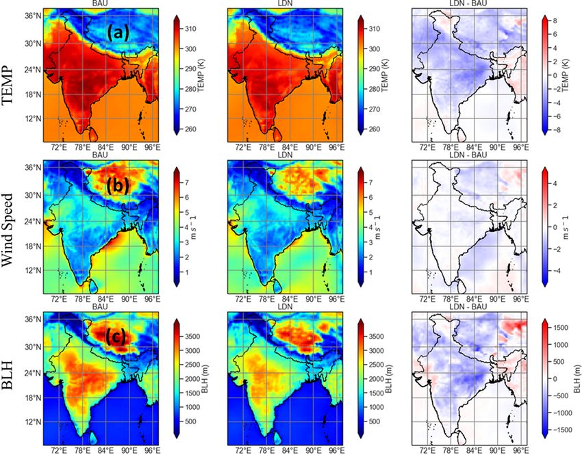
5236                                                   A. Biswal et al.: COVID-19 lockdown-induced changes in NO2 levels

   With growing scientific awareness of the adverse impacts       and the movement of the people was restricted, resulting in a
of air pollution, the number of air quality monitoring sta-       considerable reduction in the anthropogenic emissions. The
tions has expanded to over 10 000 across the globe (Ven-          restrictions were relaxed in a phased manner from the third
ter et al., 2020). Additionally, multiple satellite instruments   phase onwards in less affected areas by permitting activities
such as the Global Ozone Monitoring Instrument (GOME)             and partial movement of people (MHA, 2020).
on ERS-2, the Scanning Imaging Absorption Spectrom-                  A decline in NO2 levels over India during the lockdown
eter for Atmospheric Cartography (SCIAMACHY, 2002–                has been reported from both surface observations (Singh et
2012) on Envisat, the Ozone Monitoring Instrument (OMI,           al., 2020; Sharma et al., 2020; Mahato et al., 2020) and satel-
2005–present) on Aura, GOME-2 (2007–present) on MetOp,            lite observations (ESA, 2020; Biswal et al., 2020; Siddiqui et
and the TROPOspheric Monitoring Instrument (TROPOMI,              al., 2020; Pathakoti et al., 2020) against the previous year or
2017–present) on Sentinel-5P (S5P) have monitored NO2             average of a few previous years. A detailed study by Singh
pollution from the space for over 2 decades. Surface sites typ-   et al. (2020) based on 134 sites across India reported a de-
ically measure NO2 in concentration quantities (e.g. in units     cline of ∼ 30 %–70 % in NO2 during lockdown with respect
of µg m−3 ), but satellite NO2 measurements are retrieved as      to the mean of 2017–2019, with the largest reduction being
integrated vertical columns (e.g. tropospheric vertical col-      observed during peak morning traffic hours and late evening
umn density, VCDtrop ). The latter is preferred for studying      hours. While Sharma et al. (2020) reported a smaller de-
NO2 trends and variabilities because of global spatial cov-       crease (18 %) in NO2 for selected sites against the levels dur-
erage and spatio-temporal coincidence with ground-based           ing 2017–2019, Mahato et al. (2020) found a decrease of over
measurements (Martin et al., 2006; Kramer et al., 2008; Lam-      50 % in Delhi for the first phase of lockdown against previ-
sal et al., 2010; Ghude et al., 2011). NO2 has been reported      ous years (2017–2019), which was also confirmed by Singh
to increase in south Asian countries (Duncan et al., 2016;        et al. (2020) for the extended period of analysis. The satellite-
Hilboll et al., 2017; ul-Haq et al., 2017) and decrease over      based studies by Biswal et al. (2020) and Pathakoti et al.
Europe (van der A et al., 2008; Curier et al., 2014; Georgou-     (2020) estimated the change in NO2 levels using OMI ob-
lias et al., 2019) and the United States (Russell et al., 2012;   servations, whereas Siddiqui et al. (2020) used TROPOMI to
Lamsal et al., 2015). In the case of India, a tropospheric NO2    compute the change over eight major urban centres of India.
increase was observed during the 2000s (e.g. Mahajan et al.,      Biswal et al. (2020) reported that the average OMI NO2 over
2015), but since 2012 it has either stabilised or even declined   India decreased by 12.7 %, 13.7 %, 15.9 %, and 6.1 % dur-
owing to the combined effect of economic slowdown and             ing the subsequent weeks of the lockdown relative to similar
adoption of cleaner technology (e.g. Hilboll et al., 2017).       periods in 2019. Similarly, Pathakoti et al. (2020) reported a
However, thermal power plants, megacities, large urban ar-        decrease of 17 % in average OMI NO2 over India compared
eas, and industrial regions remain NO2 emission hotspots          to the pre-lockdown period and a decrease of 18 % against
(Ghude et al., 2008, 2013; Prasad et al., 2012; Hilboll et al.,   the previous 5-year average. Moreover, both studies reported
2013, 2017; Duncan et al., 2016). Moreover, despite the mea-      a larger reduction of more than 50 % over Delhi. Similarly,
sures taken to control NOx emissions, urban areas often ex-       Siddiqui et al. (2020) also reported an average reduction of
ceed national ambient air quality standards in India (Sharma      46 % in the eight cities during the first lockdown phase with
et al., 2013; Nori-Sarma et al., 2020; Hama et al., 2020) and     respect to the pre-lockdown phase. While recent studies have
thus require a detailed scenario analysis.                        used either only satellite observations or only surface obser-
   The nationwide lockdown in various countries during            vations, this study goes further by adopting an integrated ap-
March–May 2020, due to the outbreak of COVID-19, re-              proach by combining both measurement types to investigate
duced traffic and industrial activities, leading to a signifi-    NO2 level changes over India in response to the COVID-
cant reduction of NO2 . Studies using space-based and surface     19 pandemic using OMI, TROPOMI, and surface observa-
observations of NO2 have reported reductions in the range         tions over different regions. As both OMI and TROPOMI
of ∼ 30 %–60 % for China, South Korea, Malaysia, West-            have similar local overpass times of approximately 13:30
ern Europe, and the USA (Bauwens et al., 2020; Kanniah            (Penn and Holloway, 2020; van Geffen et al., 2020), diur-
et al., 2020; Muhammad et al., 2020; Tobías et al., 2020;         nal influences on the retrievals of NO2 for both instruments
Dutheil et al., 2020; Liu et al., 2020; Huang and Sun, 2020;      are similar. Moreover, as both instruments use nearly simi-
Naeger and Murphy, 2020; Barré et al., 2020; Goldberg et          lar retrieval schemes (i.e. differential optical absorption spec-
al., 2020) against the same period in previous years, with the    troscopy, DOAS), their NO2 measurements are believed to be
observed reductions strongly linked to the restrictions im-       comparable with a suitable degree of confidence (van Geffen
posed on vehicular movement. The lockdown in India was            et al., 2020; Wang et al., 2020). Any product differences are
implemented in various phases starting on the 25 March 2020       likely to be caused by inconsistent inputs/processing of the
(MHA, 2020; Singh et al., 2020). The lockdown restrictions        retrievals (e.g. derivation of the stratospheric slant column,
in the first two phases (phase 1: 25 March–14 April 2020          the a priori tropospheric NO2 profile, and the treatment of
and phase 2: 15 April–3 May 2020) were the strictest, dur-        aerosols/clouds in the calculation of the air mass factor; van
ing which all non-essential services and offices were closed,     Geffen et al., 2019; Lamsal et al., 2021).

Atmos. Chem. Phys., 21, 5235–5251, 2021                                             https://doi.org/10.5194/acp-21-5235-2021

A. Biswal et al.: COVID-19 lockdown-induced changes in NO2 levels                                                           5237

   We estimate the changes in the NO2 levels over differ-          for older versions by, for example, Celarier et al. (2008) and
ent land-use categories (i.e. urban, cropland, and forestland)     Krotkov et al. (2017).
and urban sizes. In addition to this, we investigate the spatial
agreement between population density and NO2 spatial vari-         2.1.2   TROPOMI NO2
ability observed at the surface. A key benefit of this study
will be to understand and assess the impact of reduced an-         TROPOMI has a nadir-viewing spectral range of 270–
thropogenic activity on NO2 levels, not only over the urban        500 nm (UV–Vis), 675–775 nm (near-infrared, NIR), and
areas but also over the rural areas (cropland and forestland).     2305–2385 nm (shortwave-infrared, SWIR). In the UV-Vis
This study thus provides an improved understanding of the          and NIR wavelengths, TROPOMI has an unparalleled spa-
spatial variations of tropospheric NO2 for future air quality      tial footprint of 3.5 km × 7.0 km, along with 7 km × 7 km in
management in India.                                               the SWIR (Veefkind et al., 2012). Details of the TROPOMI
                                                                   scheme and data are discussed by Eskes et al. (2019) and Van
                                                                   Geffen et al. (2019). The TROPOMI VCDtrop NO2 over India
2     Data and methodology                                         for the analysis period was obtained at 3.5 km × 7 km resolu-
                                                                   tion from http://www.temis.nl/airpollution/no2.php (last ac-
2.1     Data                                                       cess: 25 December 2020) and re-gridded at a spatial resolu-
                                                                   tion of 0.05◦ × 0.05◦ (∼ 5 km × 5 km) based on the gridding
Satellite observations of VCDtrop NO2 were obtained from           methodology of Pope et al. (2018). The source data are fil-
OMI (2016–2020) and TROPOMI (2019–2020). Surface                   tered to remove pixels with QA (quality assurance) values
NO2 observations (2016–2020) at 139 sites across India were        greater than 50, which removes cloud fraction less than 0.2,
from the Central Pollution Control Board (CPCB). The pe-           part of the scenes covered by snow/ice, errors, and problem-
riod from 25 March to 3 May each year is defined as the            atic retrievals (Eskes et al., 2019).
analysis period. Average NO2 levels during the analysis pe-           Although substantial differences are found between OMI
riod in 2020 and previous years are referred to as lockdown        and TROPOMI (such as the differences in the orbit and spa-
(LDN) NO2 and business-as-usual (BAU) NO2 , respectively.          tial resolution; van Geffen et al., 2020), they exhibit good
The BAU years for OMI and CPCB are 2016–2019, whereas              correlation with the surface observations (Chan et al., 2020;
for TROPOMI the BAU year is 2019 because of the unavail-           Wang et al., 2020) but are ∼ 30 % lower than the multi-axis
ability of earlier observations.                                   differential optical absorption spectroscopy (MAX-DOAS)
   NO2 data were analysed for six geographical regions             observations. Overall, TROPOMI has been reported to be su-
(north, Indo-Gangetic Plain (IGP), north-west, north-east,         perior to OMI (van Geffen et al., 2020). Detailed descriptions
central, and south) of India (Fig. S1 in the Supplement). The      of the recent retrieval schemes used for TROPOMI and OMI
NO2 changes over various land-use categories (i.e. urban,          data products are provided in van Geffen et al. (2019) and
cropland, and forestland) have been analysed using spatially       Lamsal et al. (2021), respectively. Analysis of differences be-
collocated land-use land cover (LULC) data (NRSC, 2012)            tween these two satellite data products is beyond the scope of
and OMI- and TROPOMI-observed VCDtrop NO2 . Visible                this study.
Infrared Imaging Radiometer Suite (VIIRS) fire count data
were used to study the fire anomalies during the LDN and           2.1.3   Surface NO2 concentration
other analysis periods.
                                                                   The hourly averaged surface NO2 concentration at 139 sites
2.1.1    OMI NO2                                                   (Fig. S1) for 2016–2020 across India was acquired from
                                                                   the CPCB CAAQMS (Continuous Ambient Air Quality
OMI has a nadir footprint of approximately 13 km × 24 km,          Monitoring Stations) portal (https://app.cpcbccr.com/ccr/#/
measuring in the ultraviolet–visible (UV–Vis) spectral range       caaqm-dashboard-all/caaqm-landing, last access: 1 Decem-
of 270–500 nm (Boersma et al., 2011). It uses differen-            ber 2020). The data were further quality-controlled by re-
tial optical absorption spectroscopy (DOAS) to retrieve            moving the outliers, constant values, and sites with less than
VCDtrop (i.e. VCDtrop is the difference between the to-            60 % data during the analysis period. Details of the surface
tal and stratospheric slant columns divided by the tropo-          observations are explained in Singh et al. (2020).
spheric air mass factor; Boersma et al., 2004). Here, we
use the OMI NO2 30 % Cloud-Screened Tropospheric Col-              2.1.4   Land use land cover data
umn L3 Global Gridded (Version 4) at a 0.25◦ × 0.25◦ (∼
25 km × 25 km) spatial grid from the NASA Goddard Earth            The high-resolution (50 m × 50 m) LULC data mapped with
Sciences Data and Information Services Center (GESDISC),           level-III classification for 18 major categories (NRSC,
available at (https://disc.gsfc.nasa.gov/datasets/OMNO2d_          2012) were obtained from the Bhuvan geo-platform (https:
003/summary, last access: 1 January 2021). Details of the          //bhuvan-app1.nrsc.gov.in/thematic/thematic/index.php, last
retrieval scheme and OMI data product Version 4 are dis-           access: 3 January 2020) of the Indian Space Research Or-
cussed by Krotkov et al. (2019) and Lamsal et al. (2021) and       ganisation (ISRO). To quantify the changes over urban, crop,

https://doi.org/10.5194/acp-21-5235-2021                                            Atmos. Chem. Phys., 21, 5235–5251, 2021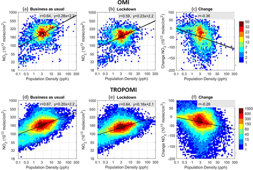
5238                                                   A. Biswal et al.: COVID-19 lockdown-induced changes in NO2 levels

and forest areas, the OMI and TROPOMI NO2 at urban grids          2.1.8    Meteorological data
(category 1), cropland (category 2 to 5), and forestland (cat-
egory 7 to 10) were extracted for further analysis. In order      The Copernicus Climate Change Service (C3S) provides the
to match the OMI and TROPOMI grid resolution with the             ERA5 reanalysis (Hersbach et al., 2020) meteorological data
Indian LULC, the dominant LULC was considered within              with an improved vertical, temporal, and spatial coverage.
the OMI and TROPOMI grid. Figure S2 shows the high-               The monthly mean meteorological data (temperature, wind
resolution LULC data used in this study for cropland, forest-     speed, and planetary boundary layer height) at 0.25◦ × 0.25◦
land, and urban areas separately. Urban areas were further di-    resolution for March, April, and May 2016–2020 were used
vided into four sizes (10–50, 50–100, 100–200, and greater        for the analysis. For details, see https://www.ecmwf.int/
than 200 km2 ) to study the change in NO2 with respect to the     en/forecasts/datasets/reanalysis-datasets/era5 (last access:
size of the urban agglomeration.                                  25 January 2021).

2.1.5   VIIRS fire counts                                         2.1.9    Analysis methodology

The VIIRS aboard the Suomi National Polar-orbiting Part-          The change in the NO2 levels for each analysis period has
nership (S-NPP) satellite provides daily global fire count at a   been calculated by subtracting the BAU NO2 from LDN
375 m × 375 m spatial resolution (Schroeder et al., 2014; Li      NO2 . We calculate the percentage change (D) using the fol-
et al., 2018). The fire count data over India during the analy-   lowing equation:
sis period from 2016 to 2020 were obtained from the FIRMS
                                                                          (LDN − BAU)
(Fire Information for Resource Management System) web             D=                  × 100.
portal (https://firms.modaps.eosdis.nasa.gov/download/, last                 BAU
access: 25 December 2020). The fire count data were grid-         The analysis was done over the whole of India as well as over
ded at 5 km × 5 km for each year by summing the fire counts       the separately considered regions and selected LULC cate-
falling on each spatially overlapping grid. The burnt area was    gories using the open-source geographic information system
calculated from the fire counts by multiplication by the VI-      QGIS.
IRS grid size (Prosperi et al., 2020).

2.1.6   Population data                                           3     Results and discussion

The gridded population density (people per hectare, pph)          3.1     Meteorological variations
data for 2020 were taken from Worldpop. (2017). World-
pop estimates the population density to be approximately          Air pollutant concentration over a region is governed by
100 m × 100 m (near the Equator) by disaggregating census         emission sources and prevailing meteorological conditions.
data for population mapping using a random forest estima-         Meteorological factors (e.g. wind, temperature, radiation,
tion technique with remotely sensed and ancillary data. De-       and rainfall) can affect the NO2 concentration (Barré et
tails of the population mapping methodology can be found in       al., 2020) as well as biogenic emissions (Guenther et al.,
Stevens et al. (2015).                                            2012). The meteorological variations between years can
                                                                  cause ∼ 15 % variations in monthly column NO2 values
2.1.7   Google mobility change                                    (Goldberg et al., 2020). However, the NO2 levels are likely
                                                                  to be similar under similar meteorological conditions. Re-
Google estimated the change in people’s movement from             cent studies (e.g. Singh et al., 2020; Navinya et al., 2020;
15 February 2020 onwards based on Google Maps informa-            Sharma et al., 2020) have shown that meteorological condi-
tion on people’s locations at places of retail and recreation,    tions remained relatively consistent over recent years during
grocery and pharmacy stores, parks, transit stations, work-       the lockdown period and therefore assumed that the changes
places, and residential places, etc. The changes were esti-       in the pollution levels during the lockdown are primarily
mated with reference to the baseline days that represent a        driven by the emission changes. However, it is important to
normal value for that day of the week. The baseline day is        highlight the meteorological differences during the study pe-
the median value from the 5-week period 3 January–6 Febru-        riod to assess the uncertainties associated with meteorologi-
ary 2020. The Google mobility change dataset provided an          cal differences.
excellent proxy for the anthropogenic activity change and            We used monthly mean ERA-5 reanalysis data (Hersbach
has therefore been used for several purposes of air quality       et al., 2020) at 0.25◦ × 0.25◦ resolution for March, April, and
studies such as lockdown emission estimation and temporal         May for BAU as well as LDN periods at the satellite local
relation with pollutant species (Archer et al., 2020; Forster     overpass time. We considered temperature (T ), wind speed
et al., 2020; Gama et al., 2020; Guevara et al., 2021) during     (WS), and boundary layer height (BLH) in our analysis. Fig-
the lockdown period of 2020. The Google mobility data and         ure 1a–c show the spatial variation in these quantities during
reports are available from Google (2020).                         BAU (left column), LDN (middle column) and the calculated

Atmos. Chem. Phys., 21, 5235–5251, 2021                                             https://doi.org/10.5194/acp-21-5235-2021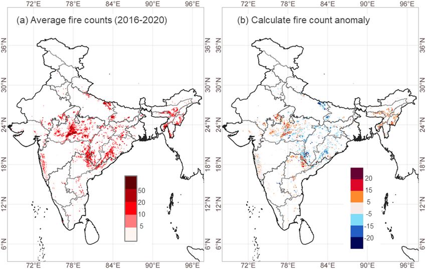
A. Biswal et al.: COVID-19 lockdown-induced changes in NO2 levels 5239
difference (LDN−BAU, right column). The probability den- widespread fire activity (counts of 10–50) is shown across
sity function (PDF) using kernel density estimation (KDE) India, such as the central region (Madhya Pradesh, Chhattis-
of the meteorological parameters is also shown (Fig. S3) for garh, Odisha), parts of Andhra Pradesh, the Western Ghats
the BAU (blue) and LDN (red). KDE is a non-parametric in Maharashtra, and the north-east region (Assam, Megha-
way to estimate the PDF. The peak of the distribution shows laya, Tripura, Mizoram, and Manipur). The fire anomaly dur-
the most probable value, and the width of the distribution ing the lockdown (Fig. 2b) shows positive fire counts (5–20)
shows the variability. The temperature difference between over the north-east region, west of Madhya Pradesh in cen-
LDN and BAU shows a slight reduction (∼ 0–3 K range) dur- tral India, and scattered locations in South India. The neg-
ing the lockdown. Wind speed values also show a reduction ative fire anomalies (−20 to −5) observed over the central
(up to 2 m s−1 ) during the lockdown, although the reduction region (Chhattisgarh and Odisha) suggest a decrease in fire
is mainly seen in certain parts of central India. Reduction in activity during the 2020 lockdown period. To minimise the
the BLH is also seen in most parts of India. In general, the impact of fire emission in our analysis, we have considered
meteorological parameters during the lockdown were simi- the grids with zero fire anomaly to assess the changes in
lar. However, the PDF (Fig. S3) during BAU and LDN shows NO2 during the lockdown. By considering the grids with zero
a small reduction (less than 5 %) in temperature and wind fire anomaly, we excluded almost all the grids which have
speed and ∼ 10 % reduction in BLH. Although small, this recorded fire activity during the analysis period. However,
weather variability can further add to the variability in the the impact of long-range transport of forest fire plumes can-
NO2 levels. However, during the lockdown in India, the NO2 not be ignored.
change was more sensitive to the emission change than the
meteorology variability. Shi et al. (2021) compared the de- 3.3 VCDtrop NO2 over India during lockdown period
trended and de-weathered change in NO2 observed over se-
lected cities in India, Europe, China, and the USA. While the The spatial distribution of VCDtrop NO2 is largely deter-
reduction in NO2 was highest for Delhi (∼ 50 %), the differ- mined by local emission sources; therefore, NO2 hotspots
ence between a detrended and de-weathered change in NO2 are found over urban regions, thermal power plants, and
observed over Delhi was much smaller (∼ 2 %) as compared major industrial corridors. For the Indian subcontinent,
to the difference calculated for other cities. This suggests that maximum NO2 is observed during winter to pre-monsoon
weather variability did not have much impact on NO2 levels (December–May) and minimum NO2 during the monsoon
over India and that most of the changes were driven by a (June–September). Region-specific peaks such as the win-
change in the anthropogenic emissions. tertime peak (December–January) in the IGP are associ-
ated with anthropogenic emissions, or the summertime peak
3.2 Fire count anomalies during the lockdown (March–April) in central India and north-east India is associ-
ated with enhanced biomass burning activities (Ghude et al.,
Forest fires are an important source of surface NO2 and 2008, 2013; Hilboll et al., 2017).
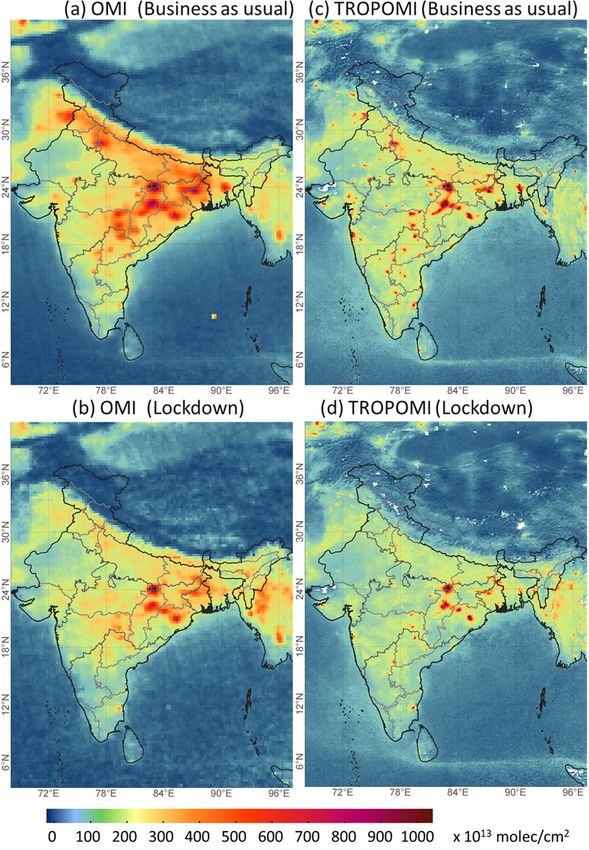
VCDtrop NO2 (Sahu et al., 2015; Yarragunta et al., 2020), We compare the LDN mean VCDtrop NO2 with the BAU
depending on the occurrence time and the intensity of fires mean for OMI and TROPOMI. The spatial distribution of
(Mebust et al., 2011). Also, as the forest fire plumes can the BAU and LDN VCDtrop NO2 observed by OMI and
be transported longer distances (Alonso-Blanco et al., 2018), TROPOMI is shown in Fig. 3a–d. The mean VCDtrop NO2
forest-fire-related NO2 can contribute to regional and global from the two instruments shows similar spatial distributions
air pollution. In India, forest fires are prevalent as 36 % during the LDN and BAU analysis period. In BAU years, the
of the country’s forest cover is prone to frequent fires, of NO2 hotspots are seen over the large fossil-fuel-based ther-
which nearly 10 % is extremely to very highly prone to fires mal power plants (∼ 1000 × 1013 molec. cm−2 ), urban areas
(ISFR, 2019). Long-term satellite-derived fire counts suggest (∼ 400–700 × 1013 molec. cm−2 ), and industrial areas. Scat-
that Indian fire activities typically peak during March–May tered sources are also present in western India, covering the
(Sahu et al., 2015), predominantly over the north, central, and industrial corridor of Gujarat and Mumbai, various locations
north-east regions (Venkataraman et al., 2006; Ghude et al., of south India, and densely populated areas (e.g. IGP). The
2013). However, the spatial and temporal distribution of fire spatial distribution showed significant changes during the
events is largely heterogeneous (Sahu et al., 2015), meaning lockdown in 2020. The details of absolute and percentage
an abrupt increase or decrease in fire activity could signifi- changes are discussed in the subsequent sections.
cantly impact NO2 levels over anomalous regions during the
lockdown. 3.4 Changes observed by OMI and TROPOMI
An investigation of fire counts during the 2020 lockdown
(LDN analysis period), when compared with the correspond- There is a substantial reduction in VCDtrop NO2 between
ing 2016–2020 average, highlights a substantial decrease the LDN and BAU (Fig. 4a and c). A large reduction in the
over the eastern part of central India and an increase over the number of hotspots, mainly urban areas, is seen in both OMI
western part of central India and the north-east. In Fig. 2a and TROPOMI observations. However, hotspots due to coal-
https://doi.org/10.5194/acp-21-5235-2021 Atmos. Chem. Phys., 21, 5235–5251, 2021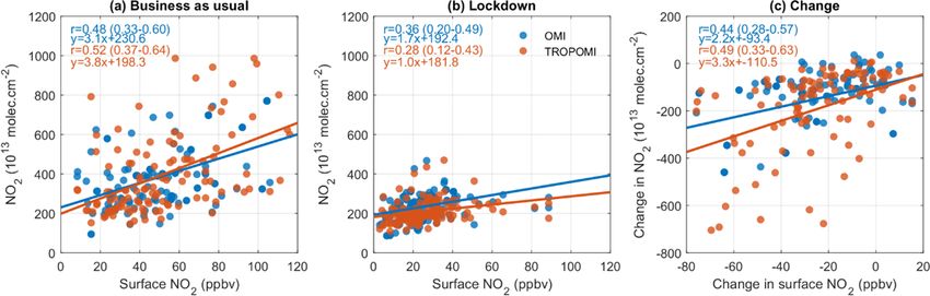
5240                                                      A. Biswal et al.: COVID-19 lockdown-induced changes in NO2 levels

Figure 1. Spatial map showing the variation in surface meteorological parameters (a temperature, b wind speed, and c BLH) from ERA-5
by comparing BAU (left column), LDN (middle column), and observed difference (LDN − BAU, right column).

Figure 2. Spatial distribution of the 5 km × 5 km gridded VIIRS fire counts. (a) Average fire counts during the analysis period (25 March–
3 May 2016–2020). (b) Gridded fire anomaly during the lockdown in 2020.

Atmos. Chem. Phys., 21, 5235–5251, 2021                                                   https://doi.org/10.5194/acp-21-5235-2021
A. Biswal et al.: COVID-19 lockdown-induced changes in NO2 levels                                                             5241

                                                                    Figure 4. (a, c) Absolute change and (b, d) percentage change in
                                                                    VCDtrop NO2 during the analysis period for LDN year compared
                                                                    to BAU years as observed by OMI (a, b) and TROPOMI (c, d).

Figure 3. Spatial distribution of mean VCDtrop NO2 (molec. cm−2 )
during the analysis period (25 March–3 May) for (a) OMI NO2 dur-    3.5     Changes in NO2 over different land use types
ing business as usual (BAU, 2016–2019), (b) OMI NO2 during the
lockdown (LDN, 2020), (c) TROPOMI NO2 during BAU (2019),            Anthropogenic NOx emissions are typically more localised
and (d) TROPOMI NO2 during LDN (2020).                              in urban and industrial centres, while biogenic sources (e.g.
                                                                    soil) are more important in rural regions. OBB activities peak
                                                                    in March–April (Sahu et al., 2015) and represent more spo-
based power plants remain during the lockdown as electricity
                                                                    radic sources. As the lockdown is expected to have reduced
production was continued. Over the NO2 hotspots, there has
                                                                    urban anthropogenic NOx sources (as shown in Fig. 4), it is
been an absolute decrease of over 150 × 1013 molec. cm−2
                                                                    important to assess the lockdown impact over the rural re-
(∼ 250 × 1013 molec. cm−2 over megacities) detected by
                                                                    gions such as cropland and forestland as well. This section
both OMI and TROPOMI. The rural VCDtrop NO2 has typi-
                                                                    estimates the changes in VCDtrop NO2 over different land
cally reduced by approximately 30–100 × 1013 molec. cm−2 ,
                                                                    types such as cropland, forestland, and urban areas (Fig. S2).
representing a percentage decrease of 30 %–50 % for OMI
                                                                    Industrial emissions are often part of the urban agglomerates
and 20 %–30 % for TROPOMI (Fig. 4b and d). For urban
                                                                    scattered around the city and are part of urban emissions. To
regions, both OMI and TROPOMI see a decrease of approxi-
                                                                    minimise the impact of OBB emissions in our analysis, we
mately 50 %, but reductions in smaller urban areas are clearly
                                                                    exclude grids with fire anomalies (Fig. 2) and those contain-
noticeable in the TROPOMI data, given its better spatial res-
                                                                    ing thermal power plants (Fig. S2d). However, absolute sep-
olution. Both instruments observe an increase in VCDtrop
                                                                    aration of the impact of long-range transportation is beyond
NO2 in the north-eastern regions and moderate enhancement
                                                                    the scope of this study.
over the western and central regions. These enhancements
are linked with the biomass burning activities during this pe-
                                                                    3.5.1    Changes over cropland and forestland
riod (Fig. 2).
                                                                    The changes in VCDtrop NO2 observed by OMI and
                                                                    TROPOMI over the cropland (Fig. S2a) in different regions

https://doi.org/10.5194/acp-21-5235-2021                                             Atmos. Chem. Phys., 21, 5235–5251, 2021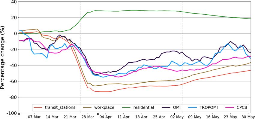
5242 A. Biswal et al.: COVID-19 lockdown-induced changes in NO2 levels
of India are shown in Fig. 5a and b and Table S1 in the as evidenced by the Google mobility reduction, which is
Supplement. A decline in VCDtrop NO2 has been observed higher for larger cities than the smaller ones (Fig. S6).
over croplands in all regions except for the north-east. A
higher percentage decline was observed over IGP and south 3.5.3 Changes over thermal power plants
regions by both the satellites. While VCDtrop NO2 has de-
creased, prominent enhancements have been observed over Thermal power plants (TPPs) are the hotspots of NO2 pol-
the north-east and few grids in central and north-west re- lution. These are scattered across the nation, with the ma-
gions. These enhancements can be attributed to the impact jority of them in Madhya Pradesh, Bihar, Uttar Pradesh,
of nearby forest fires (Fig. 2). The observed changes over Odisha, Gujarat, Chhattisgarh, West Bengal, and Tamil Nadu
the forestland (Fig. S2c) over different regions of India are (Fig. S2d). During the lockdown period, TPPs were still op-
shown in Fig. 5c–d and Table S1. The average VCDtrop NO2 erated to fulfil electricity demands. In this section, we anal-
has declined over forestland in all the regions except for the yse the changes observed over TPPs. The changes in VCDtrop
north-east, where VCDtrop NO2 was enhanced due to the pos- NO2 observed by OMI and TROPOMI over the TPPs are
itive fire anomaly (Fig. 2) during the analysis period. It can shown in Fig. S5. A decrease in mean VCDtrop NO2 levels
be noted that although we have taken the grids with zero fire over TPPs has been observed that is in line with the power
anomaly, the effect of a nearby grid exhibiting positive fire sector report, which mentions that during April 2020, en-
anomaly cannot be ignored due to atmospheric dispersion ergy demand met for India decreased by 24 % as compared to
and mixing. The inter-comparison of the changes observed April 2019 (POSOCO, 2021). Also, there is a drop (∼ 30 %)
by two satellites suggests that OMI data indicate a larger re- in thermal power production during the lockdown compared
duction in VCDtrop NO2 than TROPOMI in most of the re- to the respective period of 2019.
gions.
3.6 Inter-comparison of changes observed by OMI,
TROPOMI and surface observation
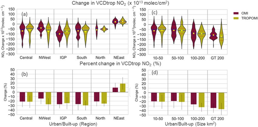
3.5.2 Changes over urban regions
Figure 7a–b show the relationship of OMI and TROPOMI
We analysed the changes in VCDtrop NO2 over the urban NO2 with surface NO2 for the BAU and LDN periods, re-
areas (Fig. S2b) in different regions of India. The calcu- spectively. During BAU, there are reasonable positive cor-
lated actual and percentage changes observed by OMI and relations between the satellite instruments and the surface
TROPOMI are shown in Fig. 6 and in Table S1. The mean sites (OMI: 0.48, 95 % CI 0.33–0.60 and TROPOMI: 0.52,
changes observed by OMI and TROPOMI show similar vari- 95 % CI 0.37–0.64). In LDN, these correlations drop to 0.36
ations in different regions. The changes observed over urban (95 % CI 0.20–0.49) and 0.28 (95 % CI 0.12–0.43), respec-
areas are larger than those observed over the forest and crop- tively. The decrease in the correlation during LDN could
lands. In contrast to the cropland and forestland, TROPOMI be due to the decrease in the signal-to-noise ratio, poten-
observed a larger reduction in VCDtrop NO2 than OMI in tially linked with the primary reduction in urban NO2 lev-
most of the regions. Densely populated IGP with the largest els. We also determined the correlation between satellite-
urban agglomeration shows the maximum change in VCDtrop and surface-observed changes during the lockdown (Fig. 7c),
NO2 followed by the central and north-west regions. The finding values of 0.44 (95 % CI 0.28–0.57) for OMI and 0.49
VCDtrop NO2 over the urban areas in the north-east region (95 % CI 0.33–0.63) for TROPOMI. This indicates that the
is likely to be influenced by the nearby forest fires through lockdown NO2 reductions appear to be present in both mea-
atmospheric dispersion and mixing, resulting in the enhance- surement types, providing us with confidence in the observed
ment of VCDtrop NO2 over the urban grids. changes detected in this study. The correlation observed over
We have also analysed the change in the VCDtrop NO2 India in this study is lower than that reported for the USA
over urban areas of different sizes. We have taken the ur- (Lamsal et al., 2015). The low correlation between OMI
ban areas of sizes more than 10 km2 and grouped them into and surface NO2 has been reported previously by Ghude et
four bins of size 10–50, 50–100, 100–200, and greater than al. (2011). While they report the temporal correlation for a
200 km2 . We then calculate the changes observed for all the single site, our study reports the spatial correlation represent-
cities filling into the respective bins. Figure 6c–d show the ing the satellites’ ability to capture the spatial heterogene-
absolute and percentage change in VCDtrop NO2 , as observed ity. One of the reasons for the lower correlation could be the
by OMI and TROPOMI, respectively. A significant reduc- choice of surface station. Generally, urban background sites
tion of 50–150 × 1013 molec. cm−2 (20–40 %) was observed are preferred for this kind of analysis. However, the surface
over the urban area of different sizes. The actual reduction in NO2 monitoring station type classification is not available for
VCDtrop NO2 is greater for the larger urban area, with peak the CPCB sites. Therefore, sites used in the analysis could be
reductions for the urban area bin (> 200 km2 ) for both OMI potentially impacted by traffic emissions, resulting in lower
and TROPOMI. The greater reduction in the larger urban ar- correlation. Another reason is that in situ measurements are
eas is mainly due to the reduction in local emission sources, more sensitive to the local emission sources than remotely
Atmos. Chem. Phys., 21, 5235–5251, 2021 https://doi.org/10.5194/acp-21-5235-2021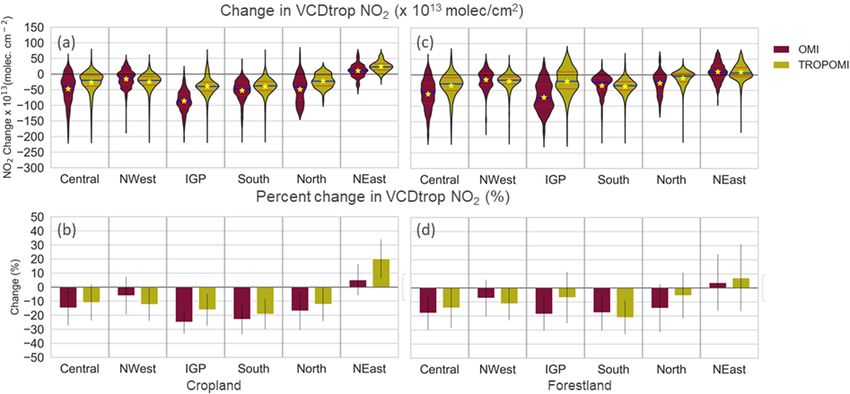
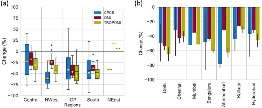
A. Biswal et al.: COVID-19 lockdown-induced changes in NO2 levels                                                                       5243

Figure 5. Observed change in VCDtrop NO2 between LDN and BAU from OMI and TROPOMI for different regions shown as (a) a violin
plot of the absolute change over cropland, (b) the percentage change over cropland, (c) a violin plot of the absolute change over forestland,
and (d) the percentage change over forestland. A violin plot is a combination of a box plot and a kernel density estimation (KDE) plot. KDE
is a non-parametric way to estimate the probability density function (PDF). The red lines in the violin plot show the interquartile range; the
blue line shows the median value; the yellow star shows the mean value. The vertical lines in the bar plot show the standard deviation. The
abbreviations NWest and NEast are for north-west and north-east regions, respectively.

Figure 6. Observed change in VCDtrop NO2 between LDN and BAU from OMI and TROPOMI for different regions shown as (a) a violin
plot of the absolute change over urban areas, (b) the percentage change over the urban area, (c) a violin plot of the observed change over
different sized urban areas, and (d) the percentage change over different sized urban areas.

sensed measurements and therefore have larger variability,               17, 15, 81, 25, and 1 for central, north-west, IGP, south,
resulting in low correlation. Proper classification of the mon-          and north-east regions (north region data not available), re-
itoring stations could provide a better assessment of satellite-         spectively. Most of the CPCB stations are in urban areas, so
based observations.                                                      our results reflect changes in predominantly urban-sourced
   The LDN NO2 percentage change, observed by surface                    NO2 . At all surface sites in all regions, there was a per-
and spatially co-located satellite measurements, is shown in             centage reduction greater than 20 % (Fig. 8a). Satellite ob-
Fig. 8a for various Indian regions. For this comparison, the             servations show a similar trend except for the north-east re-
number of available CPCB surface monitoring stations was                 gion, where enhancements are due to forest fires. Both OMI

https://doi.org/10.5194/acp-21-5235-2021                                                    Atmos. Chem. Phys., 21, 5235–5251, 2021
5244                                                    A. Biswal et al.: COVID-19 lockdown-induced changes in NO2 levels

Figure 7. Scatter plots between surface- and satellite-observed NO2 for (a) business as usual (BAU) and (b) lockdown (LDN). Panel (c)
shows a scatter plot of observed absolute change (LDN − BAU) in surface and satellite NO2 . The values shown in the brackets are the
correlation coefficients with 95 % confidence intervals (CIs).

and TROPOMI observed the highest reduction (∼ 50 %) over             2019), as shown in Fig. S4. A reduction of over 20 % was ob-
IGP. A smaller average reduction of ∼ 20 % over central In-          served in most cities except for a few in north-east and central
dia might be due to the aggregate effect of power plants, for-       India. Cities showing enhancement or smaller reductions re-
est fires, and prevalent biomass burning activities during this      flect the enhanced fire activities in the north-east and central
season. While the effect of forest fires can be observed in          Indian regions. TROPOMI can capture the reduction over the
the column NO2 , its impact on the surface NO2 is minimal.           cities near the fire-prone areas (e.g. Indore and Bhopal) be-
For the central, IGP, and south regions, the mean percentage         cause of its higher spatial resolution.
change observed by the surface monitoring station is compa-
rable to that observed by the satellites.                            3.7   Correlation of tropospheric columnar NO2 with
   We have inter-compared the percentage change in NO2 ob-                 the population density
served at the surface and satellite over the major Indian cities
(i.e. New Delhi, Chennai, Mumbai, Bangalore, Ahmedabad,              In this section, we examine the VCDtrop NO2 and pop-
Kolkata, and Hyderabad; Fig. 8b). A significant reduction in         ulation relationship for India except where fire anomalies
the range of ∼ 25 %–75 % is observed, consistent in all ob-          or large thermal power plants existed. The scatter density
servational sources used in this study. A similar reduction          plots between VCDtrop NO2 and population density for the
observed by the satellites over the cities in other parts of         BAU and LDN analysis period are shown in Fig. 9 for OMI
the world has been reported (Tobías et al., 2020; Naeger and         and TROPOMI. The data were log-transformed to establish
Murphy, 2020; Kanniah et al., 2020; Huang and Sun, 2020).            the log–log relationship as neither dataset is normally dis-
The satellites observe the largest reduction over Delhi and the      tributed. As the observed changes had negative values, this
smallest over Kolkata. While the observed decline is com-            log transformation was obtained by adding a constant value
parable for cities, Ahmedabad and Kolkata showed smaller             (Ekwaru and Veugelers, 2018), which was later subtracted
declines than observed by ground measurements. Also, the             when plotting to display the corresponding NO2 values. Both
reduction observed at the surface has a larger spatial vari-         OMI and TROPOMI NO2 show a similar relationship with
ability than the one observed from the space. This is poten-         the population density, with correlations of ∼ 0.65 during the
tially linked to the influence of the local emissions which          LDN and BAU periods, suggesting a strong dependence upon
could not be detected by the space-based instruments be-             the population (i.e. anthropogenic emissions). The slopes of
cause of relatively large satellite footprints. The results of       the lines in Fig. 9a, b, d, and e show that VCDtrop NO2 fol-
percentage change observed by OMI are consistent with the            lows a power-law scaling with population density (Lamsal et
change reported by Pathakoti et al. (2020), although Sid-            al., 2013). During BAU, the VCDtrop NO2 observed over a
diqui et al. (2020) reported a higher decline of NO2 using           grid increased by factors of 100.28 = 1.9 and 100.20 = 1.58
TROPOMI. This is because we computed the changes be-                 for OMI and TROPOMI, respectively, with a 10-fold in-
tween lockdown and BAU during the same period of the year,           crease in the population density. The rate of increase of the
whereas Siddiqui et al. (2020) estimated the changes between         VCDtrop NO2 during LDN was 100.23 = 1.7 and 100.16 =
the pre-lockdown NO2 and the lockdown NO2 , which in-                1.45 times for OMI and TROPOMI, respectively, which was
cludes the seasonal component of NO2 . We have also anal-            lower than BAU. The correlation during the LDN period was
ysed the changes in VCDtrop NO2 observed by both OMI                 marginally lower than the BAU period. This could be due to
and TROPOMI for the other major cities (Guttikunda et al.,           a larger reduction in the NO2 levels in the densely populated
                                                                     grids. The changes observed in the VCDtrop NO2 during the

Atmos. Chem. Phys., 21, 5235–5251, 2021                                                https://doi.org/10.5194/acp-21-5235-2021
A. Biswal et al.: COVID-19 lockdown-induced changes in NO2 levels 5245
Figure 8. (a) Box plot showing the percentage change between LDN and BAU in NO2 levels observed by ground and satellite measurements
at CPCB monitoring locations in different regions. (b) Bar chart showing the percentage change in NO2 levels observed in megacities in
India for the same measurements as panel (a). The vertical line in the bar chart is the standard deviation.
LDN (Fig. 9c and f) were negatively correlated (i.e. reduc- tion was higher for larger cities as compared to the smaller
tion was positively correlated) with the population density. ones (Fig. S6).
The linear relation suggests an increase in the reduction with
an increase in the population density; however, some grids 3.9 Limitations of this study
exhibit enhancements in VCDtrop NO2 due to the local emis-
sions. This study has few limitations that need to be considered
while interpreting the results. The observed changes in the
NO2 levels are the combined effect of changes in the emis-
3.8 Linking the mobility change with NO2 change sions, local meteorology, large-scale dynamics, and non-
linear chemistry. The variability in NO2 , caused by weather
patterns and non-linear chemistry is not included in the
In order to link the observed reduction in NO2 levels with present work. Our study does not distinguish the differences
the traffic emissions over the urban areas, Fig. 10 shows in the upwind and downwind transport of plumes originating
the 7 d moving average of the daily percentage change ob- from urban areas and thermal power plants. Moreover, the es-
served by OMI, TROPOMI, and CPCB across urban India timates can be biased by the forest-fire plumes, which can be
from 1 March to 31 May 2020 against the Google mobil- transported over a long distance. These limitations warrant
ity percentage reduction for three mobility categories: tran- a detailed modelling study to quantify the impact of long-
sit stations, workplace, and residential. Transit stations and range transport of plumes in the drastic reduction of urban
workplace, proxies for traffic emissions (Forster et al., 2020), emissions. One of the limitations arises due to the unavail-
show a sharp decline (∼ 70 %) due to the lockdown. The sig- ability of the surface monitoring classification according to
natures of reduced traffic can be seen even before the start its location and vicinity of the local sources, which restricted
of lockdown in mid-March 2020. The decrease in the work- a proper assessment of the space-based NO2 observation. To
places resulted in the enhancement (25 %–30 %) of people overcome this limitation, proper classification of the moni-
at a residential location. The percentage reductions observed toring stations (Geiger et al., 2013) based on the environment
by satellites and surface monitoring are consistent with each type and vicinity of the sources will be helpful in air quality
other and follow the same trend of the workplaces and tran- assessment.
sit stations. The reductions observed by satellites and surface
monitoring are ∼ 20 % lower than the reductions in work-
places and transit stations, which are compensated for by 4 Conclusions and discussion
the enhancement in residential emissions. Surface (CPCB)
measurements exhibit higher correlation (∼ 0.9 and 0.8, with The changes in NO2 levels over India during the COVID-
and without moving average) with the mobility reduction 19 lockdown (25 March–3 May 2020) have been studied
compared to the satellite observation, which has a relatively using satellite-based VCDtrop NO2 observed by OMI and
weaker correlation (∼ 0.8 and 0.5). The positive correlation TROPOMI and surface NO2 concentrations obtained from
of NO2 reduction with workplaces and transit stations sug- CPCB. The changes between lockdown (LDN) and the same
gests that the reduction observed over the urban areas was period during business-as-usual (BAU) years have been es-
linked with reduced traffic emissions due to travel restrictions timated over different land-use categories (e.g. urban, crop-
for COVID-19 containment. Moreover, the mobility reduc- land, and forestland) across six geographical regions of In-
https://doi.org/10.5194/acp-21-5235-2021 Atmos. Chem. Phys., 21, 5235–5251, 20215246 A. Biswal et al.: COVID-19 lockdown-induced changes in NO2 levels Figure 9. Scatter density plot between the VCDtrop NO2 (×1013 molec. cm−2 ) and population density (pph) for the analysis period in different years. (a) Business as usual (BAU, 2016–2019) observed by OMI; (b) lockdown (LDN, 2020) observed by OMI; (c) changes (LDN − BAU) observed by OMI; (d) BAU (2019) observed by TROPOMI; (e) LDN (2020) observed by TROPOMI; (f) LND-BAU changes observed by TROPOMI. The linear best fit lines show the log–log relationship between VCDtrop NO2 (Y ) and population density (X) given by equation y = β ·x +c, where y = log(Y ), x = log(X) and c = log(C). Therefore, the equation can be written as log(Y ) = β ·log(X)+log(C) or Y = C · X β , where β is the slope of the line. Figure 10. Temporal evolution of estimated change (7 d rolling mean) of satellite-observed VCDtrop NO2 and surface-measured NO2 for the period 1 March–31 May 2020 from the baseline. dia. Also, the changes observed from space and at the sur- agglomerations during BAU were barely noticeable during face have been inter-compared, and the correlation with the the lockdown. However, despite the reduction in electric- population density has been studied. ity production, the coal-based thermal power plants contin- Overall, a significant reduction in NO2 levels of up to ued to be major NO2 hotspots during the lockdown. Some ∼ 70 % was observed over India during the lockdown com- of the largest reductions in NO2 were observed to be over pared to the same period during BAU. The usual prominent the urban areas of the IGP region. The reduction observed NO2 hotspots observed by OMI and TROPOMI over urban for urban agglomerations was over 150 × 1013 molec. cm−2 Atmos. Chem. Phys., 21, 5235–5251, 2021 https://doi.org/10.5194/acp-21-5235-2021
A. Biswal et al.: COVID-19 lockdown-induced changes in NO2 levels                                                                5247

(∼ 30 %) and even more for megacities showing a reduc-              CDC (https://cds.climate.copernicus.eu/cdsapp, CDC, 2021). The
tion of around 250 × 1013 molec. cm−2 (50 %). The reduc-            mobility data are available on Google platform (https://www.
tion observed over the urban areas was linked with reduced          google.com/covid19/mobility, Google, 2020).
traffic emissions due to travel restrictions for COVID-19
containment. The decrease was also observed over rural re-
gions. Average declines of NO2 in the ranges of 14 %–               Supplement. The supplement related to this article is available on-
30 %, 8 %–28 %, and 10 %–24 % were observed by OMI,                 line at: https://doi.org/10.5194/acp-21-5235-2021-supplement.
and 22 %–27 %, 6 %–18 %, and 3 %–21 % were observed by
TROPOMI over the urban, cropland, and forestland, respec-
                                                                    Author contributions. AB and VS conceived the study, analysed
tively, in different regions of India. In contrast, an average
                                                                    the data and interpreted the results with SS. MPC, SSD, RJP pro-
enhancement over north-east India was observed due to pos-          vided the processed TROPOMI data and provided useful discussion
itive fire anomalies during the lockdown. Although we have          on satellite products. APK, KR, RSS, MPC, SSD, RJP, TS, SM pro-
considered the grids with zero fire anomaly during the lock-        vided useful discussion on the results. AB, VS, SS wrote the first
down, the fire emissions can still enhance NO2 levels over          draft and finalised the paper with input from all co-authors.
grids with no fire activity because of horizontal transport.
   The observed changes in VCDtrop NO2 were found to be
spatially positively correlated with surface NO2 concentra-         Competing interests. The authors declare that they have no conflict
tions, indicating that the lockdown NO2 changes appear to           of interest.
be present in both measurement types. The TROPOMI NO2
showed a better correlation with surface NO2 and was more
sensitive to the changes than the OMI because of the finer          Acknowledgements. The authors are thankful to the director, Na-
resolution. Therefore, TROPOMI can provide a better esti-           tional Atmospheric Research Laboratory (NARL, India), for en-
mate of NO2 associated with fine-scale heterogeneous emis-          couragement to conduct this research and provision of the neces-
sions. Also, VCDtrop NO2 was found to exhibit a good cor-           sary support. Akash Biswal and Shweta Singh greatly acknowl-
                                                                    edge the Ministry of Earth Sciences (MoES, India) for the re-
relation with the population density, suggesting a strong de-
                                                                    search fellowship. We acknowledge and thank Central Pollution
pendence on the anthropogenic emissions. The changes ob-
                                                                    Control Board (CPCB), Ministry of Environment, Forest and Cli-
served in the VCDtrop NO2 during the lockdown were neg-             mate Change (MoEFCC, India) for making air quality data publicly
atively correlated (i.e. reduction was positively correlated),      available. We acknowledge Bhuvan, Indian Geo-Platform of Indian
with the population density suggesting a larger reduction for       Space Research Organisation (ISRO), National Remote Sensing
the densely populated cities. However, the influence of local       Centre (NRSC), for providing high-resolution LULC data. The au-
emissions can be different in different cities.                     thors gratefully acknowledge OMI, TROPOMI, and ERA5 science
   The analysis presented in this work shows a significant          teams for making data publicly available. We also acknowledge the
change in NO2 levels across India. The observed reductions          NASA Goddard Earth Sciences Data and Information Services Cen-
can be linked with the control measures taken to prevent the        ter, Tropospheric Emission Monitoring Internet Service and Cli-
spread of the COVID-19 that restricted people’s movement,           mate Data Store. We also acknowledge Google community mobility
                                                                    data and report. We acknowledge support from the Air Pollution and
resulting in a significant reduction in anthropogenic emis-
                                                                    Human Health for an Indian Megacity project PROMOTE funded
sions. As an important message to policymakers, this study          by UK NERC and the Indian MOES (grant no. NE/P016391/1).
indicates the level of decrease in NO2 that is possible if dra-
matic reductions in key emission sectors such as road traffic
were incorporated into air quality management strategies.           Financial support. This research has been supported by the Natural
                                                                    Environment Research Council, UK (grant no. NE/P016391/1), and
                                                                    the Ministry of Earth Sciences, India.
Data availability. OMI data are available at the NASA Goddard
Earth Sciences Data and Information Services Center (GESDISC)
(https://disc.gsfc.nasa.gov/datasets/OMNO2d_003/summary, GES-       Review statement. This paper was edited by Andreas Hofzumahaus
DISC, 2021). TROPOMI data are obtained from (http://www.            and reviewed by two anonymous referees.
temis.nl/airpollution/no2.php, TEMIS, 2020). Surface measured
NO2 data across India are available at CPCB site (https:
//app.cpcbccr.com/ccr/, CPCB, 2020). VIIRS fire count data
are available at the FIRMS web portal (https://firms.modaps.
eosdis.nasa.gov/, FIRMS, 2020). India Population data used          References
in this study are available at the https://www.worldpop.org/
(https://doi.org/10.5258/SOTON/WP00532, WorldPop., 2017). The       Alonso-Blanco, E., Castro, A., Calvo, A. I., Pont, V., Mallet, M.,
LULC data for India are available at the Bhuvan, (https://bhuvan.     and Fraile, R.: Wildfire smoke plumes transport under a subsi-
nrsc.gov.in, Bhuvan, 2020) Indian Geo-Platform of Indian Space        dence inversion: Climate and health implications in a distant ur-
Research Organisation. ERA5 meteorology data are available at         ban area, Sci. Total Environ., 619, 988–1002 2018.

https://doi.org/10.5194/acp-21-5235-2021                                              Atmos. Chem. Phys., 21, 5235–5251, 2021
5248 A. Biswal et al.: COVID-19 lockdown-induced changes in NO2 levels Archer, C. L., Cervone, G., Golbazi, M., Al Fahel, N., and Hultquist, sion trends across Europe, Remote Sens. Environ., 149, 58–69, C.: Changes in air quality and human mobility in the USA dur- https://doi.org/10.1016/j.rse.2014.03.032, 2014. ing the COVID-19 pandemic, Bull. Atmospheric Sci. Technol., Duncan, B. N., Lamsal, L. N., Thompson, A. M., Yoshida, Y., Lu, 1, 491–514, https://doi.org/10.1007/s42865-020-00019-0, 2020. Z., Streets, D. G., Hurwitz, M. M., and Pickering, K. E.: A Barré, J., Petetin, H., Colette, A., Guevara, M., Peuch, V.-H., Rouil, space-based, high-resolution view of notable changes in urban L., Engelen, R., Inness, A., Flemming, J., Pérez García-Pando, NOx pollution around the world (2005–2014), J. Geophys. Res.- C., Bowdalo, D., Meleux, F., Geels, C., Christensen, J. H., Gauss, Atmos., 121, 976–996, https://doi.org/10.1002/2015JD024121, M., Benedictow, A., Tsyro, S., Friese, E., Struzewska, J., Kamin- 2016. ski, J. W., Douros, J., Timmermans, R., Robertson, L., Adani, Dutheil, F., Baker, J. S., and Navel, V.: COVID-19 as a fac- M., Jorba, O., Joly, M., and Kouznetsov, R.: Estimating lock- tor influencing air pollution?, Environ. Pollut., 263, 114466, down induced European NO2 changes, Atmos. Chem. Phys. Dis- https://doi.org/10.1016/j.envpol.2020.114466, 2020. cuss. [preprint], https://doi.org/10.5194/acp-2020-995, in review, Ekwaru, J. P. and Veugelers, P. J.: The overlooked importance of 2020. constants added in log transformation of independent variables Bauwens, M., Compernolle, S., Stavrakou, T., Müller, J.-F., Gent, with zero values: A proposed approach for determining an opti- J. van, Eskes, H., Levelt, P. F., A, R. van der, Veefkind, J. P., mal constant, Stat. Biopharm. Res., 10, 26–29, 2018. Vlietinck, J., Yu, H., and Zehner, C.: Impact of Coronavirus ESA: Air pollution drops in India following lockdown, avail- Outbreak on NO2 Pollution Assessed Using TROPOMI and able at: https://www.esa.int/Applications/Observing_the_ OMI Observations, Geophys. Res. Lett., 47, e2020GL087978, Earth/Copernicus/Sentinel-5P/Air_pollution_drops_in_India_ https://doi.org/10.1029/2020GL087978, 2020. following_lockdown, last access: 1 October 2020. Bhuvan: Indian Geo-Platform of Indian Space Research Organisa- Eskes, H., van Geffen, J., Boersma, F., Eichmann, K.-U., Apituley, tion, Thematic Services, available at: https://bhuvan.nrsc.gov.in, A., Pedergnana, M., Sneep, M., Veefkind, J. P., and Loyola, last access: 3 January 2020. D.: Sentinel-5 precursor/TROPOMI Level 2 Product User Biswal, A., Singh, T., Singh, V., Ravindra, K., and Mor, S.: COVID- Manual Nitrogendioxide, Tech. Rep. S5P-KNMI-L2- 0021-MA, 19 lockdown and its impact on tropospheric NO2 concentra- Koninklijk Nederlands Meteorologisch Instituut (KNMI), tions over India using satellite-based data, Heliyon, 6, e04764, available at: https://sentinel.esa.int/documents/247904/2474726/ https://doi.org/10.1016/j.heliyon.2020.e04764, 2020. Sentinel-5P-Level-2-Product-User-Manual-Nitrogen-Dioxide Boersma, K. F., Eskes, H. J., and Brinksma, E. J.: Error analysis for (last access: 20 December 2020), CI-7570-PUM, issue 3.0.0, tropospheric NO2 retrieval from space, J. Geophys. Res.-Atmos., 2019. 109, D04311, https://doi.org/10.1029/2003JD003962, 2004. FIRMS (NASA Fire Information for Resource Management Sys- Boersma, K. F., Eskes, H. J., Dirksen, R. J., van der A, R. J., tem): VIIRS fire count data, available at: https://firms.modaps. Veefkind, J. P., Stammes, P., Huijnen, V., Kleipool, Q. L., Sneep, eosdis.nasa.gov/, last access: 25 December 2020. M., Claas, J., Leitão, J., Richter, A., Zhou, Y., and Brunner, D.: Forster, P. M., Forster, H. I., Evans, M. J., Gidden, M. J., Jones, An improved tropospheric NO2 column retrieval algorithm for C. D., Keller, C. A., Lamboll, R. D., Quéré, C. L., Rogelj, J., the Ozone Monitoring Instrument, Atmos. Meas. Tech., 4, 1905– Rosen, D., Schleussner, C.-F., Richardson, T. B., Smith, C. J., 1928, https://doi.org/10.5194/amt-4-1905-2011, 2011. and Turnock, S. T.: Current and future global climate impacts CDC: Climate Data Store, ERA5 meteorology, available at: https: resulting from COVID-19, Nat. Clim. Change, 10, 913–919, //cds.climate.copernicus.eu/cdsapp, last access: 15 January 2021. https://doi.org/10.1038/s41558-020-0883-0, 2020. Celarier, E. A., Brinksma, E. J., Gleason, J. F., Veefkind, J. P., Cede, Gama, C., Relvas, H., Lopes, M., and Monteiro, A.: The im- A., Herman, J. R., Ionov, D., Goutail, F., Pommereau, J.-P., Lam- pact of COVID-19 on air quality levels in Portugal: A way bert, J.-C., Roozendael, M. van, Pinardi, G., Wittrock, F., Schön- to assess traffic contribution, Environ. Res., 193, 110515, hardt, A., Richter, A., Ibrahim, O. W., Wagner, T., Bojkov, B., https://doi.org/10.1016/j.envres.2020.110515, 2020. Mount, G., Spinei, E., Chen, C. M., Pongetti, T. J., Sander, S. P., Geiger, J., Malherbe, L., Mathe, F., Ross-Jones, M., Sjoberg, K., Bucsela, E. J., Wenig, M. O., Swart, D. P. J., Volten, H., Kroon, Spangl, W., Stacey, B., Ortiz, A. G., de Leeuw, F., Borowiak, A., M., and Levelt, P. F.: Validation of Ozone Monitoring Instru- Galmarini, S., Gerboles, M., and de Saeger, E.: Assessment on ment nitrogen dioxide columns, J. Geophys. Res.-Atmos., 113, siting criteria, classification and representativeness of air quality D15S15, https://doi.org/10.1029/2007JD008908, 2008. monitoring stations. JRC–AQUILA Position Paper, 2013, avail- Chan, K. L., Wiegner, M., van Geffen, J., De Smedt, I., Alberti, able at: https://ec.europa.eu/environment/air/pdf/SCREAMfinal. C., Cheng, Z., Ye, S., and Wenig, M.: MAX-DOAS measure- pdf (last access: 20 December 2020), 2013. ments of tropospheric NO2 and HCHO in Munich and the Georgoulias, A. K., van der A, R. J., Stammes, P., Boersma, comparison to OMI and TROPOMI satellite observations, At- K. F., and Eskes, H. J.: Trends and trend reversal detection mos. Meas. Tech., 13, 4499–4520, https://doi.org/10.5194/amt- in 2 decades of tropospheric NO2 satellite observations, At- 13-4499-2020, 2020. mos. Chem. Phys., 19, 6269–6294, https://doi.org/10.5194/acp- CPCB: Central Pollution Control Board, Central Control Room for 19-6269-2019, 2019. Air Quality Management – All India, Surface measured NO2 GESDISC (NASA Goddard Earth Sciences Data and Information data, available at: https://app.cpcbccr.com/ccr/, last access: 1 De- Services Center): OMI/Aura NO2 Cloud-Screened Total and cember 2020. Tropospheric Column L3 Global Gridded 0.25 degree × 0.25 Curier, R. L., Kranenburg, R., Segers, A. J. S., Timmermans, R. degree V3 (OMNO2d), available at: https://disc.gsfc.nasa.gov/ M. A., and Schaap, M.: Synergistic use of OMI NO2 tropo- datasets/OMNO2d_003/summary, last access: 1 January 2021. spheric columns and LOTOS–EUROS to evaluate the NOx emis- Atmos. Chem. Phys., 21, 5235–5251, 2021 https://doi.org/10.5194/acp-21-5235-2021
You can also read