Currency Crises in Argentina - An empirical Investigation
←
→
Page content transcription
If your browser does not render page correctly, please read the page content below
Currency Crises in Argentina
                                  An empirical Investigation
Néstor Adrián Amado
Universidad Nacional de Tucumán
nadrianamado@hotmail.com

Ana María Cerro
Universidad Nacional de Tucumán
acerro@herrera.unt.edu.ar

Osvaldo Meloni
Universidad Nacional de Tucumán
omeloni@herrera.unt.edu.ar

Abstract
This paper is aimed at studying the determinants of currency crises suffered by Argentina
from 1885 to 2003, on one hand, and at characterizing each particular currency crisis, on the
other hand.
Firstly, we look for regularities and common factors throughout history. We split the dataset
in crises and non-crises years and carried out graphical analysis in order to analyze the
behavior of key macroeconomic variables in the neighborhood of currency crises. We
complemented it by estimating a logit model including a set of variables chosen from the
prescriptions of the existing currency crises theories.
Secondly, following Kaminsky (2003) we perform regression tree analysis to classify crises
and crashes into different varieties proposed by the theories at stake. We use fifteen financial
and macroeconomic variables suggested by the empirical literature.
It is found that fiscal imbalances were always present, which is consistent with the
predictions of first generation speculative attack models. All three methods used to
characterize currency crises in Argentina show the importance of the fiscal side. Adverse
foreign factors had also a key role in explaining crises. Finally, in most of the crises,
regularities in the behavior of macroeconomic variables can be detected.

Key Words: Currency Crises, Graphic Analysis, Logit model, Regression Tree Method
JEL Classification Codes: E3, N20

                                               1
CURRENCY CRISES IN ARGENT INA.
AN EMPIRICAL IN VESTIGATION
Néstor Adrián Amado, Ana María Cerro and Osvaldo Meloni*
Universidad Nacional de Tucumán - Argentina
E-mail: acerro@herrera.unt.edu.ar; omeloni@herrera.unt.edu.ar
For historians each event is unique. Economics, however,
maintains that forces in society and nature behave in repetitive
ways. History is particular, economics is general.
Charles P. Kindleberger
Manias, Panics, and Crashes: A History of Financial Crises, 1978.
En la historia monetaria argentina, a pesar de su confusa
apariencia, nótese una serie de períodos de ilimitada confianza y
prosperidad, de expansión en las transacciones, de
especulación inmobiliaria y fantasía financiera, seguidos de
colapsos más o menos intensos, precipitados en pánicos que
originan la liquidación forzada de las operaciones, el
relajamiento de la confianza, la postración y el estancamiento de
los negocios. Sin duda, cada uno de estos ciclos no se
presentan exactamente en las mismas condiciones, ni con
idéntico carácter, pero, considerados en conjunto, es posible
encontrar en ellos, hechos fundamentales que se repiten, cuyo
análisis permite formular síntesis acerca de su evolución ...
buscaremos demostrar que en nuestras crisis, aparte de las
diferencias de menor cuantía, interviene un factor fundamental,
... y peculiar al grado de formación histórica del país.
Raúl Prebisch
Anotaciones sobre nuestro medio circulante (1921)
I. IN T R O D U C T I ON
When it comes to currency crises, Argentina is one the most interesting cases to study. Not
only had a larger number of crises years than any other developed and emerging country, as
documented by Eichengreen and Bordo (2000), but also was the protagonist of some of the
more resounding cases of crises and default in the world history. Not only is one of the most
*
We thank Gustavo Adler, Horacio Aguirre, Manuel Luis Cordomí, Víctor Elías, Lucas Llach, Saúl Lizondo and
José Pineda for helpful comments to earlier versions of this paper. All remaining errors are ours. We gratefully
acknowledge the support of the Consejo de Investigaciones de la Universidad Nac ional de Tucumán (CIUNT)
Grant 26/F 204. The views expressed herein are those of the authors and not necessarily those of the CIUNT.
2vulnerable countries to international and regional crisis as shown by Kaminsky and Reinhart
(2002) but also generated its own currency crisis.
The cost of several crises and crashes for Argentina, in terms of real output losses, has been
huge, and possibly one of the largest in the world. The latest crash in 2001/ 2002, known as
Tango, brought about a 15% decrease in real GDP and pushed vast sectors of the
population below the poverty line. Similarly, the 1989 crash, which ended in hyperinflation,
resulted in a 9% fall in real GDP.
According to Cerro and Meloni (2004), who work with monthly data from 1885 to 2003, there
were 19 crises in 118 years of history, which implied 32 crisis years. That is, Argentina had a
crisis year every 3.7 years. It seems very difficult to match that record.
What are these crises caused by? Do they always recognize the same causes? Which are
the “fundamental facts” repeated in every crisis, mentioned by Prebisch in the opening
quotation at the epigraph? To put it in another way, did Argentina suffer from the same
disease throughout history? Were there different varieties of the same disease? Is there any
particular deficiency in the immunological system of Argentina that makes the country prone
to currency crises? What was the role of external shocks in the crises?
This paper is not aimed at answering all these questions but at studying the determinants of
the 19 currency crises suffered by Argentina from 1885 to 2003, on one hand, and at
characterizing each particular currency crisis, on the other hand.
Firstly, we look for regularities and common factors throughout history. We split the dataset
in crises and non-crises years and carried out graphical analysis in order to analyze the
behavior of key macroeconomic variables in the neighborhood of currency crises. We
complemented it by estimating a logit model. As in Frankel and Rose (1996) we include four
groups of explanatory variables attempting to characterize Argentina’s currency crises.
Variables were chosen from the prescriptions of the existing currency crises theories.
Secondly, following Kaminsky (2003) we perform regression tree analysis to classify crises
and crashes into different varieties proposed by the theories at stake. We use fifteen financial
and macroeconomic variables suggested by the empirical literature.
While the first approach misses the details but highlights the repeated facts, the regularities;
the second approach, stresses diversity, the characteristics that make each crisis a unique
historic event.
The remainder of the paper is organized as follows. Section II sketches some theoretical
issues on currency crises. In Section III we briefly survey the empirical literature on the topic.
Section IV explains the empirical results obtained from the graphic analysis, the logit analysis
and the regression tree. Finally, section VI presents some conclusions, conjectures and
guidelines for further research.
II. M O D EL S OF C U R R EN C Y CR I SE S
Since the pioneer contribution of Krugman (1979), the family of currency crises models has
grown in such a way that we already have three generations. The first-generation models,
associated, precisely, to the name of Krugman showed how inconsistencies between
domestic economic conditions and the exchange rate commitment lead to the collapse of the
currency peg. In his paper, budget deficit fully monetized is financed by Central Bank
expending reserves. With the exchange rate fixed, investors get rid of the excess money
supply by exchanging domestic currency for foreign reserves of the central bank. When such
reserves fall to a critical threshold, a speculative attack is launched, causing reserves
depletion and the abandon of the exchange rate peg.
The speculative attack takes place when the shadow price of exchange rates (the price that
would prevail after the speculative attack takes place) equals the exchange rate. At that
3moment reserves are driven to zero forcing the abandonment of the fixed exchange rate, and
the economy switches to a floating rate regime. With reserves depleted, budget deficit is
financed by money creation, which in turn causes an increase in inflation rate.
Two important aspects of this model should be remarked: the first one is that speculative
attacks are not only possible, but also inevitable when fiscal policy is not consistent with the
exchange rate regime. The time in which the speculative attack will take place is perfectly
known forehand, so nobody is taken by surprise. Secondly, there is no incompatibility
between rational behavior and the (apparent) arbitrariness of currency attacks. Rational
economic behavior, characterized by smoothly evolution over time, can be associated with
dramatic attacks and changes in the exchange rate regimes.
S e c o n d-G e n e r a t i o n M o d e l s
The so– called second generation models developed by Flood and Garber (1984b) and
Obstfeld (1986, 1994) became widely recognized after the canonical crisis model failed to
explain the European Monetary System crises (1992-1993). Second generation models are
based on the existence of multiple equilibria. When investors anticipate that a successful
attack will alter policy (even if they agree that currency policy may be consistent with the
currency peg) it will be expected that future fundamentals (conditional on an attack’s taking
place) be incompatible with the peg. In this case, government might defend the currency, but
the costs (high interest rate, high unemployment rate) can be so onerous that government
finally devaluates, so the market anticipates that action and acts in advance.
The government compares the net benefits from changing the exchange rate versus
defending it. Policymakers usually have as many good reasons to defend the fixed exchange
rate but also to abandon it. For example, if government has a large debt burden denominated
in domestic currency, devaluation would evaporate part of the debt. Or, if the country is
suffering high unemployment rates, and nominal wages are rigid, devaluation would diminish
real wages. But, on the other hand, in inflation-prone countries a nominal anchor is a
guarantee against high inflation rates, so defending the currency keeps inflation under
control. Another argument put forward to resist devaluations is that a fixed exchange rate
facilitates investment and international trade. Crucially, the cost of defending a fixed
exchange rate increases when people expect that the regime will be abandoned.
Models of self-fulfilling attacks imply that good fundamentals are not enough neither to
prevent attacks, nor to avoid a currency crisis. The state of fundamentals determines the
existence and multiplicity of attack equilibrium. In Krugman’s model fundamentals may be
consistent with exchange rate or not. In second generation models the same is true for
extreme values of fundamentals, but there’s also a large middle ground over which
fundamentals are neither so strong as to make crises inevitable nor so weak as to make an
attack impossible. An important difference between this two models is that in the first the
moment of the depletion of reserves can be anticipated, while in the second the timing is
undetermined, so it can happens unexpectedly, and that is why they are considered so
dangerous.
Third Generation Models
The Southeast Asian currency crisis in 1997 was the starting point for a new theory of
currency crises. As Krugman (1998) points out, none of the fundamentals that led to a first
generation crisis were present in the Asian economies. Asian economies did not face severe
unemployment when the crisis begun, nor had any incentive to abandon the peg to carry out
expansive monetary policy. Besides, in all count ries were present a boom-bust cycle in the
asset markets. Financial intermediaries had a central role in the crisis. A mismatch in the
deposits of the banking and non-banking system was present: the institutions borrowed
short-term money, often in foreign currency, and lent that money in long-term domestic
currency.
The conventional currency crisis theories associated with inconsistency in present or future
fundamentals missed the role played by financial intermediaries whose liabilities were
4perceived to have government guarantee, but were essentially unregulated and therefore
subject to moral hazard problems.
The evidence seems to suggest that Asian crisis was neither the consequence of fiscal
imbalances, nor were the incentives to follow an expansive monetary policy, but were the
problems with financial intermediaries that drove the crisis. The excessive risk lending led to
inflation in the asset prices. When the crisis burst, the asset prices fall, the insolvency of
intermediaries were visible, forcing them to cease operations, which in turn implied further
deflation in asset prices.
Sudden Stop Models
The sudden stop theory of currency crises emphasizes the liquidity problem in emerging
economies due to a sudden stop, that is, episodes of sudden and massive reversal in capital
inflows. The reversions generally happen in countries that have experienced heavy capital
inflows and consequently important current account deficits. To face this sudden capital
outflow, governments spend reserves, which increases financial vulnerability and finally
devaluates its currency. The resulting reverse in current account deficit impacts on economic
activity and employment. This line of research is only recent and is associate to the works of
Calvo (1998), Calvo and Reinhart (2000) and Calvo, Izquierdo and Talvi (2002)
I I I. E M P I R I C A L LI TE R A T U R E
The numerous empirical researches on currency crises focused on two types of studies: (a)
the analysis of specific events or particular countries and, (b) cross-country analysis. They
are mainly dedicated to:
• Analysis of the probability of crises
• Test for contagion and determining the channels through which contagion occurs
• Establish the relationship between currency and banking crisis
• Comparison of historic and recent crises
• Test for specific theories of what causes crises in a given country or group of
countries.
Table 1 summarizes some of the most relevant papers in the recent empirical literature.
In general, the empirical literature works with stylized models having the following as main
predictions:
• In first-generation models, previous to the speculative attack we should observe an
expansive fiscal and monetary policy, and a decline in international reserves for long
periods.
• On the other hand, second generation models imply that speculative attacks should be
followed by expansive monetary and fiscal policies.
• Third generation models emphasize the role played by financial intermediaries, so they
analyze variables related to them, such as the liquidity coefficient, solvency of the
financial sector, external debt maturity, and assets denomination versus liabilities.
5Table 1. Empirical literature
Authors Period Countries
Blanco and Garber (1986) 1973-1982 Mexico
Cumby and Wijnbergen (1989) Dec 1978- -April 1981 Argentina
Eitchengreen, Rose and Wyplosz 1967-1992 22 Emerging and developed countries suffering a
(1994) crisis
Klein and Marion (1994) 1957-1991 -Monthly data Panel data for 16 Latin American countries
Pazarbasioglu and Otker (1994) 1979-1993 - Monthly data Denmark, Ireland, Norway, Spain and Sweden
Calvo and Mendoza (1996) 1994-1995 Mexico
Eitchengreen, Rose and Wyplosz 1959-1993 –quarterly data 20 industrialized countries
(1996)
Frankel and Rose (1996) 1971-1992 105 countries
Sachs, Tornell and Velasco (1996) 1994/1995 20 emerging economies
Flood and Marion (1997) January 1957-January 1991 80 episodes of fixed exchange rate in 17 Latin
American countries
Burnside, Eichenbaum and Rebelo July 1995-May 1998 Indonesia, Malaysia, Thailand, Korea, Philippines,
(1998) Hong Kong, Singapore and Taiwan
Chang and Velasco (1998) 1987-1997 Indonesia, Korea, Malaysia, Philippines, Thailand,
Mexico, Argentina, Brazil and Chile
IMF (1998) 1975-1997 50 industrialized and emerging countries
Kaminsky, Reinhart and Lizondo 1970-1995 15 developed and 5 developing countries
(1998)
Berg and Pattillo (1999) 1997 Asian countries
Glick and Rose(1999) 1971, 1973, 1992-1993, 161 countries affected by crises
1994-1995, 1997-1998
Kaminsky and Reinhart (1999) Crisis 1997 Asian countries
Tornell (1999) 1985-1995 Hong Kong and 22 emerging countries
Kaminsky and Reinhart (2000) 1997-1999 - daily data 35 countries
Moreno and Trehan (2000) 1974-1997 post Bretton 121 countries
Woods
Eichengreen and Bordo (2002) 1883-1998 21 emerging and developed countries
Kaminsky, Reinhart and Vegh (2002) 1826-2002 Countries affected by different crises
Kaminsky (2003) 1970-2002 20 countries
Crises in Argentina
Cerro and Meloni (2003) dated 19 crises throughout 118 years of history. Five crises were
rated as “crashes”, nine as “mild” and five as minor turbulences. Interestingly, the number
and magnitude of the crises increases through time (see Table 2). The five “deep crises”
identified correspond to the years, 1890-91, 1929-32, 1975-76, 1989-91 and 2001-02.
Crises were determine by means of a Market Turbulence Index (MTI) which is the sum of
changes in three variables: the exchange rate, international reserves and the interest rates
weighted by the inverse of their variability. The index stems from the idea that market
pressure increases when exchange rate devaluates (rises), when interest rates increase and
when international reserves fall. Under a floating exchange rate regime, we expect abrupt
increases in the exchange rate as crisis develops, while under a fixed exchange rate, prior to
devaluation, interest rates increase and international reserves diminish.
Whenever the MTI is greater than the mean (µ) plus k standard deviations (STD), a “signal”
or “turbulent episode”. is identified. An episode is considered a deep crisis or “crash” when
two “close” months with MTI greater than the mean value plus three STD is observed. On the
other hand, If the MTI is greater than µ plus two STD but less than µ plus three STD, we call
it “mild crisis”. If MTI exceeds its mean value in a half STD at least twice the episode is
considered “minor turbulence”. The remaining episodes, i.e. when the index departs less
6than one half standard deviation from the average are termed as “non- crisis” or tranquility
times.
Table 2. Crises Summary
Number of GDP Growth Type of Crisis
Number of Crises Years
Years (annual
Period crises crises as % of total Deep Minor
(1) average Mild
(2) years (3) years (3)/(1) (crash) Turbulence
in%)
1885 -
29 2 4 13.8 5.4* 1 1 0
1913
1914 -
32 4 8 25.0 3.1 1 1 2
1945
1946 – 31 7 10 32.3 3.8 1 4 2
1976
1977 –
15 4 9 60.0 0.4 1 2 1
1991
1992-
11 2 3 27.3 2.1 1 1 0
2002
Total 118 19 34 28.8 3.3 5 9 5
The 19 crises implied 34 crises years. That is, 29% of the 118 were crisis years, which meant
one crisis year every 3.5 years. A given year is considered a crisis year if the market
turbulence index exceeds one standard deviation from the average in at least 2 months,
consecutive or alternate (no more than six months apart).
According to them Market Turbulence Index, the most turbulent period of Argentina’s history
was 1977 –1991, not only because it registered 4 crises in 15 years, but also because nine
of those years were crisis years, which meant 60% of these years in crisis (see Appendix,
Table 2 A for details).
IV. E M P I R I C A L R E S U LT S
Macro variables Behavior in the Neighborhood of the crisis: Graphic Analysis
How did the Argentine economy perform in the neighborhood of crises? Is there any
regularity in the behavior of the macroeconomic variables around these extreme episodes?
In order to approach to the answer of these questions we carried out Graphic Analysis for
several macroeconomic variables. That is, we put a magnifier on the behavior of macro
variables three years before and three years after each crisis. That is, for each of the 19
crises identified for Argentina, we normalize all the variables in the dataset in seven periods:
t-3; t-2; t-1; t; t+1; t+2; t+3, with t standing for the peak of the crisis. We report the average
value of the variables and the intervals (in color lines) resulting from adding and subtracting
one standard deviation.
As Frankel and Rose (1996) point out, a graphical approach has advantages and
disadvantages. Among the first, it imposes no parametric structures on the data, it makes
only a few assumptions that are necessary in inference statistics, and it is often more
accessible and informative than tables with estimations of coefficients. On the other hand,
the graphic analysis is informal, and intrinsically univariate.
7The various graphs show dramatic differences in the behavior of all variables examined
before, during and after the crises 1. A brief comment on each variable follows.
• Excess real M1 as percentage of the GDP peaks in t-1 (4.1% on average), falls during
crisis at 0.5% and reaches a trough at t+1, averaging –3.9. This variable was built as
deviations from the estimated demand for money (in real terms) as % of GDP.
• Public Expenditure Growth: peaks two periods before the crises (on average, increases
8.7%) and the trough at t+1 with an average value of 0.4% (which means a fall of 8.3%)
0.4 30
0.3
20
0.2
0.1 10
0.0 0
-0.1 1 2 3 4 5 6 7 t-3 t-2 t-1 t t+1 t+2 t+3
-10
-0.2
-0.3 -20
Excess Real M1/GDP Public Expenditure Growth
• Fiscal Deficit (as % of GDP) starts it upward path before crises and peaks during crises
at an average level greater than 4%, showing the lack of funds (both, external as well as
internal) to finance the fiscal gap.
• International Reserve Growth: increases at t-3 (about 30%), then starts to fall and
reaches a minimum at t with a fall of -11%
10 100
80
8
60
6 40
4 20
0
2 -20 t-3 t-2 t-1 t t+1 t+2 t+3
0 -40
t-3 t-2 t-1 t t+1 t+2 t+3 -60
-80
Fiscal Deficit (% of GDP)
International Reserves Growth
• Exports growth reaches a peak two years before crises (on average 22.5%), while the
trough happens at the moment of the crises with a value of –0.2%. The fall at t migh be
the result of unfavorable TOT but also a consequence of uncertainty about future rules of
the game.
♦ Imports growth is highly correlated wikt GDP movements. its maximum rate of growth is
reached one period before crises, with 31.2% and its minimum during crises, with a
negative rate of growth of -11.7%.
♦ Current Account Deficit (as % of GDP) reaches a peak at t-1 (average -2.3) and a trough
at t (-0.38%), i.e. an improvement of 2%. That is, during crises the lack of capital inflows
leaves the country with no other alternative than adjusting aggregate demand.
1
Similar conclusions are drawn by Cerro and Meloni (2003) by means of non-parametric tests, such as
Kolmogorov—Smirnov, that tests for the equality of distribution and Kruskal-Wallis, Wilcoxon, Median Chi- Square
and Van der Waerden testing for equality of population between crisis and tranquil periods.
850 100 0.04
40 80 0.02
30 60 0.00
20 t-3 t-2 t-1 t t+1 t+2 t+3
40 -0.02
10
20 -0.04
0
t-3 t-2 t-1 t t+1 t+2 t+3 0 -0.06
-10
-20 t-3 t-2 t-1 t t+1 t+2 t+3
-20 -0.08
-30 -40 -0.10
Exports Growth Imports Growth Current Account Deficit (as % of GDP)
• GDP growth reaches a peak two years before the beginning of crises (on average 5.7%)
and the trough at the moment of the crises (-3.6% on average). The difference between
peak and trough is 9.3% on average.
• Real Exchange Overvaluation:, built as deviation from the RER trend, accumulates
pressure during t-2 and t-1 and overshoots at t right after the devaluation.
15 160
4
10
2 120
5
0
80
t-3 t-2 t-1 t t+1 t+2 t+3 0
-2
t-3 t-2 t-1 t t+1 t+2 t+3
-4 -5 40
-6 -10
0
-15 t-3 t-2 t-1 t t+1 t+2 t+3
Real Exchange Rate Overvaluation Terms of Trade
GDP Growth
• Real M3 growth falls abruptly during crises reaching a value of –10.5% on average, after
peaking two periods before crises with a value of 7.6% on average
• Banking crises, taken from Kaminsky and Reinhart (2000), always precede or coincide
with currency crises.
• Money Multiplier m2, reaches a peak two periods before crises and troughs two periods
after crises with values of 1.11 and 1.03 respectively.
30 0.80
20 0.60 1.7
10
0.40
0
1.3
-10 t-3 t-2 t-1 t t+1 t+2 t+3 0.20
-20 0.00
0.9
-30 -3 t +3
-0.20
-40
-0.40 0.5
Real M3 Growth Banking Crisis money
-3 t multiplier m2 +3
• International Rate of Interest: it reaches a peak one period before the crises begin. For
emerging economies, the increase in the international interest rate is very important for
two reasons. Firstly, it is key to explain the capital inflow and outflow to emerging
countries as pointed out by Calvo, Reinhart and Leiderman (1992). Secondly, it impacts
on the service of external debt. An increase in the rate of interest is associated with
9worsening in quasi fiscal deficit and consequently in fiscal accounts. In most severe crisis
adverse external conditions were present.
9
8 6000
7
4000
6
5 2000
4
3 0
2 t-3 t-2 t-1 t t+1 t+2 t+3
1 -2000
0
-4000
t-3 t-2 t-1 t t+1 t+2 t+3
Public External Debt (Changes)
Rate of Interest - Libor
Finally, the components of the Market Turbulence Index behave as expected. That is.
Exchange rate depreciates very slowly in t-2 and t-1 and explodes at t.
Regression Analysis
Following Frankel and Rose (1996), we try to characterize Argentina’s currency crises rather
than testing specific theories of crises.
We estimate a logit model whose binary dependent variable takes the value 0 for no-crises
years, and 1 for crises years. Independent variables were classified into three groups: (i)
Domestic Macroeconomic Indicators: real public expenditure growth, GDP growth, Real
M3 growth. (ii) External Indicators: CAD, Reserves/Imports Ratio, Real Exchange Rate
Overvaluation, External Debt. (iii) Foreign Variables: TOT, International Rate of Interest.
Three alternative models were estimated using maximum likelihood 2. Results are tabulated in
Table 3. Since logit coefficients are not directly interpretable, we report the effect of a change
in variables on the probability of crisis. We also tabulated z-statistics with null hypothesis of
no effect and report McFadden R squared.
Most of the variables included are statistically significative at usual levels. It is found that the
probability of crisis increases when GDP, real M3 growth, and the ratio reserves to imports
fall. Crises are also more likely when the local currency appreciates (lagged once), and TOT
impairs (although this variable is not statistically significative at standard values in models 2
and 3).
On the other hand, an increase in public expenditure growth, in the current account deficit
(lagged one period), in the external debt (not significative in Model 1), and an increase in the
international rate of interest also increase the probability of crisis.
Interestingly enough, the results of the regression let us conclude that fiscal variables have
an important role in determining the probability of crisis. The domestic macroeconomic
effects, measured by GDP growth and real M3 growth are very strong. An appreciation of the
currency (lagged once) also increases the probability of a cri sis, but contemporaneously it
has the opposite sign as expected, since during crisis devaluation has already taken place.
However we can also see that an impairing of external conditions (measured by an increase
in international rate of interest or by a wo rsening in TOT) makes a crisis more probable.
Table 3. Regression Results.
2
We also estimated by probit and Linear Probability Model, but results do not differ significantly
10Variable Model 1 Model 2 Model 3
3.90 -0.93 -0.85
C
(1.18) (-0.27) (0.25)
-0.17 -0.17 -0.17
GDP growth
(-2.99) (-2.76) (2.76)
0.05 0.04 0.04
Public expenditure growth
(2.55) (2.29)
-0.08 -0.09 -0.08
Real M3 growth
(-2.79) (-2.60) (2.60)
-6.05E-06 1.45E-05
External Debt
(-0.06) (0.13)
-0.06 -0.03 -0.03
Terms of Trade (TOT)
(-2.10) (-1.14) (-1.18)
-4.90
Current Account Deficit
(-0.78)
-22.41 -22.22
Current Account Deficit (-1)
(-2.39) (-2.41)
0.23
LIBOR
(1.19)
0.56 0.55
LIBOR (-1)
(2.37) (2.36)
-1.62 -1.42 -1.41
Reserves /Imports
(-2.13) (-2.07) (-2.04)
0.41 0.44 0.44
Real Exchange Rate overvaluation
(2.51) (2.59) (2.60)
-0.47 -0.48 -0.48
Real Exchange Rate overvaluation (-1)
(-2.31) (-2.28) (-2.28)
LR statistic (11 df) 52.67285 60.28001 60.26328
Probability (LR stat) 8.56E-08 3.21E-09 1.19E-09
McFadden R-squared 0.42324 0.484366 0.484
Obs with Dep=0 92 92 92
Obs with Dep=1 26 26 26
Note: Z statistic in parenthesis below coefficient
Regression Tree Analysis
Regression Tree Analysis is a non-parametric device, aimed at identifying the characteristics
of each crisis separately. This well-known method in many disciplines (see details in
Appendix), was introduced in the analysis of currency crises by Kaminsky (2003).
The regression tree method applied to currency crises has a couple of advantages when
compared to other traditional methods. First, it does not impose the same functional form to
all crises such as logit and probit models. Second, the probability of crises augments as the
number of variables indicating vulnerability increase. For example, an expanding domestic
credit may be explosive with convertibility and with capital inflow reversal.
The output of regression tree method is a set of terminal nodes, each one characterizing a
crisis or a group of crises. The method considers an initial split of the data into two
subgroups according to the rule of minimum node. Many different criteria can be defined for
selecting the best split at each node. However, the properties of the final tree selected are
insensitive to the choice of splitting rule. Variable misclassification costs and prior
distributions can be incorporated into the splitting structure in a natural way.
11This split is repeated in sequential form until each subset terminates either when there is no
impurity reduction from splitting or when the number of observations in the cell is less than a
specified number of rows.
The classification tree resembles the one obtained using the Akaike information criterion
(Venables and Ripley, 1996). The key features of the tree approach are: (1) Splits are
sequential, so that only a subset of all possible splits is examined. (2) Cross-validation is
used to asses model fit. (3) No penalty value is assigned a priori; rather, all possible
penalties are considered. (4) It makes powerful use of conditional information in handling
nonhomogeneous relationships. (5) It does automatic stepwise variable selection and
complexity reduction. (6) It is invariant under all monotone transformations of individual
ordered variables. (7) It is extremely robust with respect to outliers and misclassified points in
the learning sample. (8) It handles missing values through the use of surrogate splits.
The method can uncover general forms of nonlinearity in data; Brieman et al. (1984) shows
that the classification tree method is consistent in the sense that, under suitable regularity
conditions, the risks of partition-based predictors and classifiers converge to the risk of the
corresponding Bayes rules.
Empirical Results
Previous to running the Regression Tree method, we classified years of crises and non-
crises during 118 years of argentine history according to the MTI. We did not distinguish
among crises intensity, i.e. deep, mild and minor turbulences. Indicators of crises were
grouped according to the prescription of the first, second, third generation models and
sudden stops. A total of fifteen indicators were used.
Table 4. Indicators of Currency Crises Models
Model of Currency Crises Variables
First Generation Models Fiscal Deficit (% GDP)
Public Expenditure Growth
Excess Real M1 Balances/GDP
Second Generation Models Exports Growth
GDP Growth
Real Exchange Rate Overvaluation
Current Account Deficit
Third Generation Models M2/Reserves Growth
M2 Multiplier Growth
M2/Reserves
M2 Multiplier
Bank Deposits Growth
Debt External Debt/Exports
Sudden Stop Nominal Libor
Nominal Libor Growth
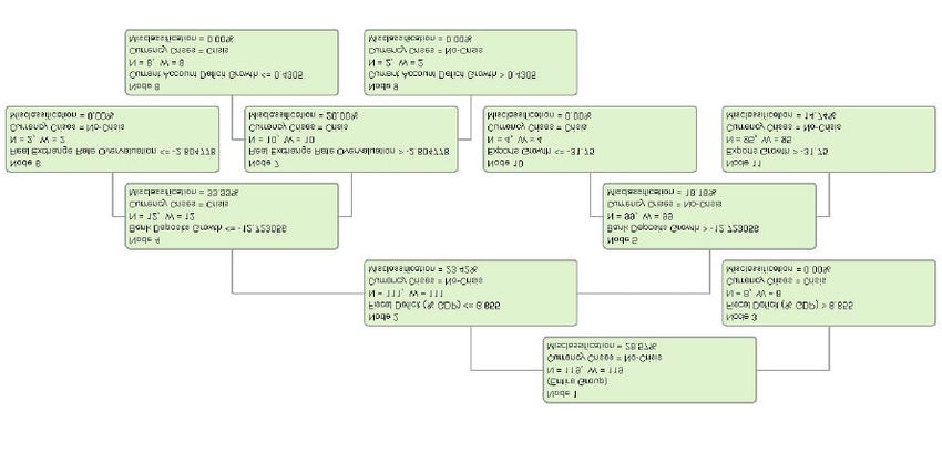
12The results of regression tree are reported in Figure 1. They show the criteria for splitting the
sample. The 34 years of crises were classified in different varieties of currency crises
according to only five indicators (among the fifteen listed in table 4): Fiscal Deficit, Real
Deposits, Overvaluation, Exports and Current Account Deficit. The overall importance of
variables is presented in Table 1A.
It is found that observations are assigned to six terminal nodes, which let us classify the
crises into three different groups. The first split of the data is carried out on the fiscal deficit
as percentage of GDP, with a threshold of 6.6. For values greater than that, we identify eight
crisis years. This variety of crises is consistent with first generation models.
For values minor than 6.6, there is a new split in the subgroup, performed by real total
deposits. If its rate of growth is greater than -12.7, the new split comes from exports, and we
have another final node with four crises.
If real deposits grow less than -12.7%, the sample is split again by the variable overvaluation.
If there is a RER overvaluation greater than -2.6, and changes in Current Account Deficit are
less than 0.4, we find another terminal node with eight crises.
Table 2A describes the characteristics of the final group. There we can identify indicators of
vulnerability. In the first node (number 3) the only indicator of vulnerability is fiscal deficit,
there are eight years of crises where fiscal deficit as percentage of GDP is greater than
6.6%. These crises correspond to the following years (see Table 3A): 1958, 1962, 1975 and
76 and 1981 to 1985.
Node 8 is related to an important fall in real deposits jointly with an impairing in current
account deficit not greater than 0.43 and an overvaluation greater than -2,6. In that final node
we find the following crises years: 1890, 1891, 1914, 1951, 1989, 1990, 1995 and 2001.
Notice that node 8 includes the most severe crises Argentina went throughout its history.
Node 10 is related with a considerable fall in exports. We identify this node with the following
crises: 1921, 1930, 1938 and 1949. These crises are also consistent with a fall in Terms of
Trade, which worsen the prices of exports, a fall of the international demand for Argentineans
products or with a fall in production of primary goods, associated with climatological
phenomenon.
The results obtained so far are quite preliminaries. Future research is necessary, basically in
improving the data set in two directions. The first one is related to increase the number of
indicators variables to be used, for example we need better indicators of external debt,
domestic credit, among others. The second one is related to broaden the period or periodicity
of the data. One possibility is to look for date during XIX century; other possibility is to find
quarterly data for the whole period. The increase in the sample would be necessary to
assure consistency.
However, even preliminary, some conclusions may be drawn. The first one is that extremely
high fiscal deficit is responsible for eight currency crisis in Argentina. The second one is that
worsen in external conditions may have deleterious consequences in Argentina, mainly when
domestic imbalances are present. The third one, when many indicators of vulnerability are
signaling crises, they are almost inevitable.
13Figure 1
Regression Tree Analysis
14V I. C O N C L U S I O N S
This paper explores the determinants and characteristics of currency crises in Argentina
throughout 118 years of history. Taken the 19 crises dated by Cerro and Meloni (2004) as a
group, the graphic analyses favor the predictions of the first generation model of currency
crisis. In fact, the observed behavior of Real Public Expenditure, Fiscal Deficit, the Rate of
growth of International Reserves and Excess Real M1 coincide with the ones expected from
the Krugman model. However, the behaviors of the other variables analyzed suggest that
some factors associated to second-generation models like the overvaluation of the domestic
currency, and the fall in GDP and exports before crises were also important. Likewise, the
expansion of Money Multiplier M2 and the precedence of Banking Crisis to currency crises
speak about the presence of variables related to third-generation model. Similarly, the
behavior of LIBOR and the reversion in the current account supports the sudden stop theory.
The logit estimation confirmed that domestic macroeconomic effects, measured by GDP
Growth and Real M3 Growth, and Public Expenditure Growth were very strong. An
appreciati on of the currency (lagged once) increases the probability of crisis and impairing of
external conditions also make a crisis more probable.
The regression tree method classifies argentine crises into three subgroups: one with Fiscal
Deficit as a key variable, which supports the first-generation model prediction and reinforces
our previous findings. Another subgroup features, besides Fiscal Deficit, RER overvaluation,
and a fall in Real Deposits, which indicates a complex mix of factors associated to first,
second and third generation models. The last subgroup is characterized by RER
overvaluation, diminishing Real Deposits and reversal in capital flows captured by the
variable Current Account Deficit.
With all this evidence at hand, some preliminary conclusions can be drawn:
• Fiscal imbalances were always present, which is consistent with the predictions of first
generation speculative attack models. All three methods used to characterize currency
crises in Argentina show the importance of the fiscal side.
• In most of the crises, regularities in the behavior of macrovariables can be detected. In
that sense, Prebisch was right
• Adverse foreign factors had also a key role in explaining crises: an increase in
international rate of interest that affects the direction of capital flows and an impairing in
TOT increases the probability of crisis.
Although most of the evidence presented here supports mainly the first generation
speculative attack models or à la Krugman, we also detect some elements of sudden stop
theory and third generation models.
The severity and persistence of currency crises in Argentina, the high vulnerability to external
shocks regardless of the type of government (de facto or constitutional) and the political party
in office, seem to reveal problems at the roots of the country rather than associated to
particular economic policies or specific adverse shocks. It all seems to point out at the
institutional design.
15REF ER E N C E S
Agenor, Pierre-Richard, Bhandari, Jagdeep and Flood, Robert (1992) Speculative attacks and models
of balance-of-payment crises. Staff Papers, Vol. 39.
Blanco, Herminio and Garber, Peter (1986). Recurrent devaluations and speculative attacks on the
Mexican Peso. Journal of Political Economy, Vol. 94 (1), pp. 148-166.
Bordo, Michael and Vegh, Carlos (1998) What if Alexander Hamilton had been Argentinean. A
comparison of early monetary experiences of Argentina and the United States. NBER Working Paper
Nº 6862.
Breiman, Leo, Friedman, Jerome, Olshen, Richard and Stone, Charles (1984) Classification and
regression trees. Wadsworth & Brooks. California.
Calvo, Guillermo and Fernández, Roque (1982) Pauta Cambiaria y Déficit Fiscal in Fernández, R. and
Rodriguez, C. (Editors) Inflación y Estabilidad. Ediciones Macchi, Buenos Aires.
Cerro, Ana María (1999) La conducta cíclica de la economía Argentina y el comportamiento del dinero
en el ciclo económico. Argentina 1820-1998. Tesis de Magíster inédita (Universidad Nacional de
Tucumán)
Cerro, Ana María y Meloni Osvaldo (2003) Crises in Argentina: 1823-2002. The Same Old Story?,
Anales de la XXXVIII Reunión Anual de la Asociación Argentina de Economía Política, Mendoza. Web
Site: www.aaep.org.ar
Cerro and Meloni (2004) Determinants of Currency Crises in Argentina: 1885 – 2003 . Trabajo
presentado en las XIX Jornadas de Economía Banco Central del Uruguay. Web Site: www.bcu.gub.uy
Cortés Conde, Roberto (1989) Dinero, Deuda y Crisis. Evolución Fiscal y Monetaria en al Argentina.
Buenos Aires. Editorial Sudamericana
Cumby, Robert and Sweder van Wijnbergen (1989) Financial Policy and Speculative Runs with a
crawling peg: Argentina 1979-1981. Journal of International Economics. Vol. 27
Delargy, P.J.R. and Goodhart, Charles (1999) Financial crisis: plus ça change, plus c’est la même
chose. Financial Market Group. Special Paper # 108.
della Paolera, Gerardo and Taylor, Alan (2000) Economic Recovery from the Argentine Great
Depression: Institutions, Expectations, and the Change of Macroeconomic Regime. NBER Working
Paper No. w6767.
Diz, César (1970) Money and prices in Argentina: 1935 –1962, in Varieties of Monetary Experience.
D. Mieiselman Editor. Chicago: University of Chicago Press.
Dornbusch, Rudiger (1984) Argentina since Martínez de Hoz . NBER Working Paper # 1466.
September.
Edwards, Sebastián (1993) Devaluation controversies in the developing countries, in Bordo and
Eichengren (eds.) A Retrospective on the Bretton Woods System, Chicago.: University of Chicago
Press
Edwards, Sebastián (1989) Real Exchange Rate, Devaluation and Adjustment: Exchange Rate Policy
in Developing Countries. Cambridge: MIT Press.
Eichengreen, Barry, Rose, Andrew and Wyplosz, Charles (1994) Speculative attacks on pegged
exchange rates: an empirical exploration with special reference to the European monetary system .
NBER Working Paper # 4898.
Eichengreen, Barry, Rose, Andrew and Wyplosz, Charles (1996) Contagious currency crises. NBER
Working Paper # w5681.
Eichengreen, Barry and Bordo, Michael (2002) Crises Now and Then: What lessons from the Las Era
of Financial Globalization? NBER Working Paper # 8716.
Gerchunoff, Pablo and Llach, Lucas (2003) El Ciclo de la Ilusión y el Desencanto . Editorial Ariel.
Buenos Aires.
16Fernández, Roque (1982) Consideraciones ex – post sobre el Plan Económico de Martínez de Hoz , in
Fernández, R. and Rodriguez, C. (Editors) Inflación y Estabilidad. Ediciones Macchi, Buenos Aires
FIEL (1989) El Control de Cambios en la Argentina. Editorial Manantial. Buenos Aires.
Flood, Robert and Garber, Peter (1984). Gold monetization and gold discipline. Journal of Political
Economy, Vol. 92, pages 90-107.
Friedman, Milton and Schwartz, Anna (1963a), A Monetary History of the United States: 1867-1960.
Princeton. Princeton University Press
Friedman, Milton and Schwartz, Anna (1963b) Money and Business Cycles. Review of Economics and
Statistics, Vol. 45, Nº 1, part 2, supplement (February)
García, Valeriano (1973) A Critical Inquiry into Argentine Economic History. Unpublished dissertation.
University of Chicago.
Girton, Lance and Roper, Don (1977) A Monetary Model of Exchange Market Pressure Applied to
Postwar Canadian Experience. American Economic Review. Vol. 67.
Grilli, Vittorio (1990) Buying and Selling attacks on Fixed Exchange Rate Systems. Journal of
International Economics. Vol. 20.
Krugman, Paul (1979) A model of balance of payment crises. Journal of Money, Credit and Banking.
Vol. 11, pages 311-325.
Obstfeld, Maurice (1986) Rational and self-fulfilling balance of payment crises. American Economic
Review. Vol. 76, pages 72-81.
Obstfeld, Maurice (1994) The Logic of Currency Crises. NBER Working Paper 4640
Prebisch, Raúl (xxx) Anotaciones sobre nuestro medio circulante. A propósito del último libro del
doctor Norberto Piñero.
Reinhart, Carmen and Kaminsky, Graciela (1999) The Twin Crises: the causes of banking and
balance-of-payment problems. American Economic Review. Vol 89, Nº 3, June.
Salant, Stephen and Henderson, Dale (1978) Market Anticipation of Government Policy and the Price
of Gold. Journal of Political Economy. Vol. 86.
Taylor, Alan (1994) Three Phases of Argentine Economic History. NBER Working Paper No. h0060.
Taylor, Alan (1997) Argentina and the world capital market: saving, investment and international
capital mobilityin the twentieth century. NBER Working Paper No. 6302.
Taylor, Alan (1998) On the costs of inward looking development. Price distortions, growth and
divergence in Latin America. Journal of Economic History. Vol. 57
17APPENDIX
CLASSIFICATION TREES.
This appendix describes the construction of a classification tree. The method can uncover
general forms of nonlinearity in data; Brieman et al. (1984) shows that the classification tree
method is consistent in the sense that, under suitable regularity conditions, the risks of
partition-based predictors and classifiers converge to the risk of the corresponding Bayes
rules.
Define the measurements (x1, x2, …, xr) made on a case as the measurement vector x
corresponding to the case. Take the measurement space X to be defined as containing all
possible measurement vectors. Suppose that the cases or objects fall into J classes; that is,
C = {1, …, J}. Based on these measurements, the goal is to find a systematic way of
predicting what class is in. A systematic way of predicting class membership is a rule that
assigns a class membership in C to every measurement vector x in X. That is, given any x ∈
X, the rule assigns one of the classes {1, …, J} to x. A classifier or classification rule is a
partition of X into J disjoint subsets A1, …, Aj, X = ∪j Aj such that for every x ∈ Aj the
predicted class is j.
The first problem in the construction is how to use a learning sample to determine the binary
splits of X into smaller and smaller pieces, beginning with X itself. The fundamental idea is to
select each split of a subset so that the data in each of the descendant subsets are “purer”
than the data in the parent subset. Various criteria have been proposed for evaluating splits,
but they have all the same basic goal which is to favor homogeneity within each node child
and heterogeneity between the child nodes. The goal of splitting is to produce child nodes
with minimum impurity.
The classification tree algorithm is as follows:
(1) For each of the variables xi, i = 1, …, r, consider an initial split of the data into two
subgroups according to the rule minimum node, or equivalently tree, impurity with estimated
class probabilities p(j/t), j = 1, …, J
i(t) = ö (p(1/t), …, p(J/t)) (1)
Many different criteria can be defined for selecting the best split at each node, i.e. Gini and
towing. However, the properties of the final tree selected are insensitive to the choice of
splitting rule. The Gini criterion, considered slightly better than towing by Brieman et al
(1984), has the form
i(t) = Ój i p(j/t) p(i/t)
where variable misclassification costs and prior distributions can be incorporated into the
splitting structure in a natural way. The xi and the split that minimize (1) define the initial split
of the data into two subgroups which we call S1 y S2; denote this set of splits as T1.
(2) Repeat step 1 on each of the two sets S1 and S2. The minimum impurity for observations
in S1 will define two new groups S3 y S4; S5 and S6 are constructed for observations in S2.
Notice that new splits may occur on different variables, i.e. j k. Denote this new set of splits
S3 … S6 as T2. Repeat again for each of these new subsets and generate a new set of splits
T3. As before, the splits in T3 define disjoint subgroups of data. Sequential splitting of each
subset terminates either when there is no impurity reduction from splitting or when the
number of observations in the cell is less than a specified number of rows.
(3) The initial tree generated by step 2 is larger than as the data splits were costless. We
now “prune” the tree by incorporating a cost to data splits. Let the cost of splitting equal α
#(N), where #(N) is the number of terminal nodes in a tree. For each α 0, one determines
which set of terminal nodes minimizes
18Rα (T) = R (T) + α #(N)
Thus, Rα (T) is formed by adding to the misclassification cost of the tree a cost penalty for
complexity. If α is small, the penalty for having a large number of terminal nodes is small and
T(α) will be large. As the penalty α per terminal node increases, the minimizing subtrees T(α)
will have fewer terminal nodes. Finally, for α sufficiently large, the minimizing subtree T(α)
will consist of the root node only, and the tree T max will have been completely pruned.
Although α runs through a continuum of values, there are at most a finite number of subtrees
of Tmax. Thus, the pruning process produces a finite sequence of subtree T 1, T2, T3, … with
progressively fewer terminal nodes.
(4) Calculate a cross-validated estimate of the R (T) for each subtree T1, T2, T3, … Then, the
subtree with the smallest cross-validated R (T) produces the right sized tree.
The classification tree resembles one which chooses among different splits using the Akaike
information criterion (Venables and Ripley, 1996). The key features of the tree approach are:
(1) Splits are sequential, so that only a subset of all possible splits is examined. (2) Cross-
validation is used to asses model fit. (3) No penalty value is assigned a priori; rather, all
possible penalities are considered. (4) It makes powerful use of conditional information in
handling nonhomogeneous relationships. (5) It does automatic stepwise variable selection
and complexity reduction. (6) It si invariant under all monotone transformations of individual
ordered variables. (7) It is extremely robust with respect to outliers and misclassified points in
the learning sample. (8) It handles missing values through the use of surrogate splits.
Program
The program used to build the right tree was DTREG (Decision Tree Regression Analysis
For Data Mining and Modeling) by Phillip H. Sherrod. Copyright © 2003-2004. All rights
reserved. www.dtreg.com.
Variables
Target: Currency Crisis (Deep, Mild and Turbulence)
Predictors:
Fiscal Deficit (% GDP)
Public Expenditure Growth
Excess Real M1 Balances/GDP
Bank Deposits Growth
Real Exchange Rate Overvaluation
M2/Reserves Growth
M2 Multiplier Growth
M2/Reserves
M2 Multiplier
GDP Growth
Exports Growth
External Debt/Exports
Current Account Deficit
Current Account Deficit Growth
Nominal Libor
Nominal Libor Growth
19Tree fitting algorithm: Gini.
Assumed prior probabilities for target categories: P (Crisis) = 0.25
Misclassification costs: Equal misclassification costs for all categories (crisis and no-crisis).
How to classify rows with missing predictor values: Surrogate predictors
Method for testing and pruning the tree: 10-fold cross-validation.
The pruning control: Prune to minimum cross-validated error.
Table 1A. Overall Importance of Variables
Variable Importance
Fiscal Deficit (% GDP) 100%
Exports Growth 71%
Bank Deposits Growth 65%
Current Account Deficit Growth 45%
M2 Multiplier Growth 33%
M2 Multiplier 33%
M2/Reserves 26%
Real Exchange Rate Overvaluation 22%
Libor Growth 16%
Current Account Deficit 14%
M2/Reserves Growth 13%
GDP Growth 10%
Public Expenditure Growth 5%
100%
90%
80%
70%
Importance of Variables
60%
50%
40%
30%
20%
10%
0%
Fiscal Deficit (% Exports Growth Bank Deposits Current Account M2 Multiplier M2 Multiplier M2/Reserves Real Exchange
GDP) Growth Deficit Growth Growth Rate
Overvaluation
20Table 2A. Varieties of Currency Crises
Group Group Group Predicted
Node Characteristics Misclassification
1 2 3 Value
3 Fiscal Deficit (% GDP) > 6.65 * Crisis 0%
Fiscal Deficit (% GDP)You can also read